Cartesian Genetic Programming for Trading: A Preliminary Investigation

(1)

Cartesian Genetic Programming for Trading: A Preliminary

Investigation

Michael Mayo

School of Computing and Mathematical Sciences University of Waikato, Hamilton, New Zealand

Abstract

In this paper, a preliminary investigation of Cartesian Genetic Programming (CGP) for algorithmic intra-day trading is conducted. CGP is a recent new vari-ant of genetic programming that differs from tradi-tional approaches in a number of ways, including be-ing able to evolve programs with limited size and with multiple outputs. CGP is used to evolve a predic-tor for intraday price movements, and trading strate-gies using the evolved predictors are evaluated along three dimensions (return, maximum drawdown and recovery factor) and against four different financial datasets (the Euro/US dollar exchange rate and the Dow Jones Industrial Average during periods from 2006 and 2010). We show that CGP is capable in many instances of evolving programs that, when used as trading strategies, lead to modest positive returns. Keywords: Cartesian Genetic Programming, Algo-rithmic Trading, Rule Learning

1 Introduction

Algorithmic trading is the problem of automating de-cisions to buy and sell financial assets such that, even after trading costs and losses are taken into account, the cumulative net return from the decision series is positive. The main tasks of these decision strate-gies are (i) market direction prediction and (ii) po-sition sizing, risk management, and entry/exit man-agement. The main problem with task (i), of course, is that markets are notoriously difficult to predict. In fact, there is a long history of debate about the efficient market hypothesis (Fama, 1970) and the is-sue of whether or not market price movements are essentially random walks (see, for example, Beechey et al. (2000) for a recent counter-analysis). In spite of this, past research efforts from computer scien-tists appear to show that pattern recognition tech-niques such as machine learning can make profits in the markets. Recent examples include the works of Contreras et al. (2012), Lean and Lai (2007), Liu and Xiu (2009), Ni and Yin (2009), Barbosa and Belo (2008), Hirabayashi et al. (2009), and Larkin and Ryan (2010).

Putting aside the debate for a moment, task (ii) mentioned above (which is concerned with the details about whether to act on a prediction and if so, how to

Copyright c2012, Australian Computer Society, Inc. This pa-per appeared at the 10th Australasian Data Mining Conference (AusDM 2012), Sydney, Australia, December 2012. Confer-ences in Research and Practice in Information Technology (CR-PIT), Vol. 134, Yanchang Zhao, Jiuyong Li, Paul Kennedy, and Peter Christen, Ed. Reproduction for academic, not-for-profit purposes permitted provided this text is included.

act) is also not without its difficulties. For example, a market may be quiet one day and volatile the next. Therefore a strategy that that assigns a large posi-tion size to a trade on the quiet day (where the risk is low) may be in violation of its own risk management rules if it assigns the same position size the follow-ing day (where the risk is higher due to an increased likelihood of sharp price movements). Markets be-haviours are well known to be non-stationary series (Sewell, 2011) and therefore methods and strategies that worked in the past cannot be expected to con-tinue working. Furthermore, non-stationarity applies not just to prices but also to other important fac-tors such as volatility and seasonal aspects (where seasonality includes not only properties that change with an annual cycle but also those that follow in-traday, time-of-day-based cycles and weekly cycles). Non-stationarity probably explains why some techni-cal strategies that traditionally worked in the past now may no-longer yield profits.

This paper takes the view that intraday market prices may be predictable to a small degree, although that “edge” may be very slim indeed. Financial en-gineering may be required to actually make such pre-dictions profitable. We also take the stance that due to non-stationarity, a large amount of past training data isnot required for learning trading strategies – in fact, too much data may lead to problems such as the learning of patterns that are now defunct. We therefore, in our experiments, use two months of in-traday data to learn a trading strategy, and test it on the following month of intraday data.

The machine learning method of choice in this paper is Cartesian Genetic Programming (CGP) (Miller, 2011). We chose this method for a num-ber of reasons. Firstly, CGP evolves programs that can have a fixed upper limit on size because they are represented as a fixed-size array. In contrast, tradi-tional tree-based Genetic Programming methods have no limit on size and the problems of bloat are well known. Secondly, CGP can evolve programs with multiple outputs as well as multiple inputs. Although we do not use more than one output in the exper-iments presented here, in the future this would be advantageous for learning trading strategies because the multiple outputs can be used to emit different as-pects of the strategy. For example one output may be a prediction of direction, and the second output may be a position size indicator (with a zero indicat-ing “no trade”). A third output could possibly be a distance to a stop loss price.

The third and final reason for CGP being inter-esting from a trading perspective is that as learning proceeds over time (in generations), programs tend to reduce in complexity whenever fitness hits a plateau (Miller, 2011). That is, in the absence of further

(2)

im-provements, CGP programs tend to have less active nodes due to the genetic drift feature of CGP. For a trading strategy, this is a very desirable property be-cause smaller programs are easier for humans to un-derstand, making them more like “traditional” indi-cators. Furthermore, smaller programs are less prone to overfitting.

2 Background

In this section, a brief review is given of the important concepts used in this paper. In particular, we describe the CGP approach used, and overview the important financial ideas.

2.1 Cartesian Genetic Programming

CGP is a relatively new field of genetic programming. It has found application in areas either where there is a significant amount of low-level data to be pro-cessed (e.g. in the evolution of image processing filters (Sekanina et al., 2011a)) or where the programs must adhere to significant physical constraints (e.g. the layout of circuits on a board (Sekanina et al., 2011b)). Financial applications are more related to the image processing scenario, because a trading strategy can be thought of as a “filter” on data that produces an output (that being signal to trade or not to trade), where the data is not 2D image data but is instead a stream of historical 1D price series data.

The canonical CGP algorithm (described more fully in (Miller, 2011)) is defined as follows. Firstly, a small number of fixed parameters must be speci-fied. The first is the population size popsize, which in canonical CGP is set to 5. This very small popula-tion size is offset by the fact that it is customary for CGP to run for a very large number of generations,

maxgens, which may have a value in the millions. Further parameters describe the fixed features of each program, such as the number of inputs, nin; the number of outputs, nout; and the maximum number of function call instructions (ornodes) in a program,

nl. Typically there also needs to be a fixed arity

parameter that specifies the number of inputs each function/node takes. We also in this research fix the number of point mutations per offspring to nm,

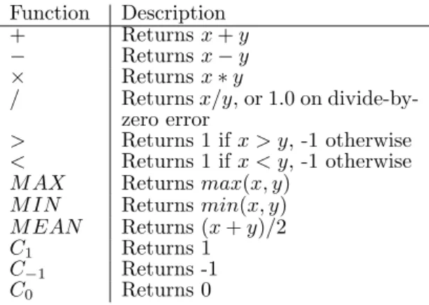
al-though in general this parameter need not be fixed. Next, a tableF unctions must be defined. A pro-gram in CGP is defined as a linear array of func-tion calls of lengthnl. Traditionally, basic numerical functions such as addition, subtraction, sin, cosine, square root, etc are used; alternatively, if the domain is logic circuits, low level AND and OR gates are sen-sible choices for functions. In our domain, we are interested in learning programs that resemble finan-cial indicators, so the functions chosen are similar to the basic components used in those traditional indi-cators, such as comparison (greater than, less than, min, max), basic arithmetic operators, and the mean function. We also include functions that use none of their inputs at all, but instead have a fixed constant output such as 1 or -1. These resemble “bias” nodes from neural networks and often have an impact on the performance of CGP. The complete list of functions used in this paper are given in Table 1.

Once the parameters and F unctions table have been specified, the next step is to give the algorithm a value functionF itness() with which to evaluate each individual program. The basic CGP algorithm can then proceed, and it does so as a simple 1 +λ evo-lutionary strategy (Miller, 2011) where λ = 4. In

Table 1: Functions used to construct individual pro-grams. Functions either take two inputsxand y, or they ignore the inputs and produce a constant value.

Function Description

+ Returnsx+y

− Returnsx−y

× Returnsx∗y

/ Returnsx/y, or 1.0 on divide-by-zero error > Returns 1 ifx > y, -1 otherwise < Returns 1 ifx < y, -1 otherwise M AX Returnsmax(x, y) M IN Returnsmin(x, y) M EAN Returns (x+y)/2 C1 Returns 1 C−1 Returns -1 C0 Returns 0

other words, the search starts from randomly gener-ated programs, and proceeds generationally. In each generation, only the best program is retained and the others in the population are replaced by mutated off-spring of the best program. There is no crossover in canonical CGP.

One interesting facet of the algorithm that differ-entiates CGP from other evolutionary algorithms is its method of selecting the parent for the next gen-eration. In CGP, an offspring replaces its parent if its fitness is greater than or equal to its parent’s fit-ness. That is, even if there is no improvement in fitness, the search algorithm can adopt a new “best program” and parent for the next generation as long as the offspring’s fitness is at least equal to its par-ents. This mechanism permits neutral mutations that allow for genetic drift, a feature that adds random di-versity into the population without any cost. It has been shown previously such diversity significantly im-proves the search performance of CGP.

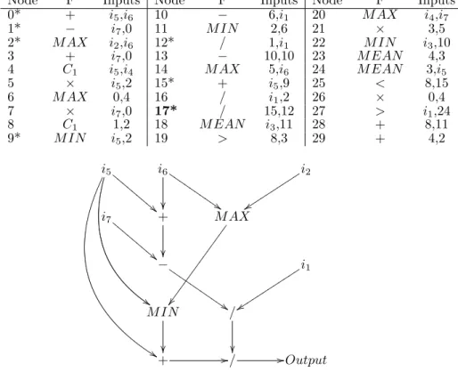
An example of a program evolved using CGP in the experiments reported here is shown in Figure 1.

This example illustrates the phenomenon of non-coding regions in CGP quite well. Each node/function call in a program may be coding or non-coding. If a node is defined as coding, this means that it is connected to the inputs either directly or in-directly. In the case of indirect connection, the con-nection is via the outputs of another function. Fur-thermore, in order to be a coding node, the node’s own output must also be used to compute the final outputs of the program. Any other function nodes are essentially useless and constitute “junk” regions of the genotype. In Figure 1, the example program has 7 coding and 23 non-coding function nodes. Note that CGP programs are directed acyclic graphs as op-posed to trees or linear sequences of instructions.

2.2 Financial Concepts

The main financial trading concepts will be explained briefly in this subsection.

The first important concept to understand is the notion that assets can be bought andsold as well as sold short. Short selling is different from selling an asset that you already own, because rather than re-ducing your (positive) quantity of the asset by selling it, you actually sell your asset first (i.e. acquire a negative quantity of the asset) and gamble that the price will go down so that you can buy it back later

(3)

at a lower price, thus making a profit. Short sell-ing is therefore the opposite of normal “long” buysell-ing and selling. In all of our experiments we assume that a trading strategy can both buy long and sell short, and that a trade (buying or selling) is closed with the opposite action.

Another important concept to understand is the way that trading strategies are evaluated. Whereas normal machine learning classifiers are evaluated via standard measures such as accuracy or ROC, in fi-nance these concepts have very little relevance if the strategy’s financial performance is also not consid-ered. For example, a strategy with a 60% accuracy rate in picking direction will consistently lose money if its average loss per trade in dollar terms is twice its average win, even though the accuracy is greater than random.

We therefore utilise in this research the following three measures of a trading strategy’s performance: cumulative return, i.e. the sum of the consecutive small wins and losses that a strategy makes over its testing period; maximum drawdown, which is defined as the maximum drop in cumulative return over the same period; and recovery factor, which is defined as the ratio of the first of these quantities to the second. To illustrate, suppose that a strategy yields a profit of $50 in the first week, but loses it all plus a further $25 in the second week (yielding a balance of $-25). In the third week, the strategy earns $35 profit, thus ending the three weeks with a $10 profit. The cumulative return in this case is $10; the maxi-mum drawdown is $75; and the recovery factor is $10_$75 or 0.133.

Note that the recovery factor essentially nor-malises the return against maximum drawdown; strategies with both high returns and drawdowns should yield the same recovery factor as those with low returns but correspondingly low maximum draw-downs. A negative recovery factor indicates that the strategy made a loss, while a recovery factor of less than 1 indicates that the strategy’s drawdown was greater than its eventual profit. Strategies with a re-covery factors of 1 or more are therefore desirable.

3 Experimental Setup

In this section, the datasets used in the experiments are described. We then move on to outlining the way in which CGP programs were evaluated for fitness estimation purposes.

3.1 Datasets

Four datasets from two different major markets were utilised in our evaluation of CGP for trading strategy learning. The two markets selected were deliberately chosen because they are highly liquid, meaning that there is simply a larger number of traders. The “herd-ing behaviour” of the crowd may therefore more easily become apparent in these markets. Smaller markets, on the other hand, are less liquid and therefore more prone to sudden large price movements arising from single trades and other such noise. The two markets that we chose are quite disparate in order to ensure that our approach was tested rigorously.

The chosen markets were (i) the market for US currency, as determined by the Euro/US dollar ex-change rate, and (ii) the US share market, as mea-sured by the Dow Jones Industrial Average. Both markets have quite different characteristics. We also chose two quite distinct time-periods from their mar-ket price series, namely pre-recession 2006 and

post-recession 2010. The two time periods combined with the two markets yielded four datasets.

Each dataset consisted of three month’s worth of data, of which the first two months were used for training and the last month for out-of-sample test-ing. The exact dates and details of the datasets are given in Table 2.

The data we used is available from a financial data firm, Pi Trading1 _{and comes in the form of an}

EST time-stamped series of open, high, low and close prices for every minute that a market is open. There are no records for minute bars where there are no transactions (i.e. where the open, low, high and close values are identical), so the actual number of records in the dataset is less than the number of minutes that the markets were open for. For the exchange rate data, this amounts to about 80,000 minute records in both the 2006 and 2010 periods, and for the Dow Jones data (which is open during US business hours only) this comprises approximately 25,000 records.

3.2 Trading Simulation using CGP Programs

In order to evaluate a trading strategy with historical data, it must be simulated. However, a simulation of a trading strategy can only ever be a rough approxi-mation, simply because real trading has many other factors that are beyond the scope of a simulation. For example, brokers usually charge transaction costs on trades, but the charging scheme may vary from bro-ker to brobro-ker and across time. Likewise, live data may contain errors that are subsequently cleaned in historical datasets. Historical data also does not con-tain information about slippage and other order fill-ing problems. In the simulations described here, we assume no transaction costs and that there are no complications with order filling such as slippage or incorrect prices.

Given the assumptions, each CGP program was evaluated in the following way. The data (either the in-sample split during learning or the out-of-sample split during testing) was divided into days. It was as-sumed that each strategy would make one trade per day, at the start of the day, and that the trade would remain open until the last minute of same day. At that point it would be closed and the cumulative re-turn or loss of the strategy updated. We do not sim-ulate position sizes in these experiments – instead, the cumulative return is measured in points, which are a standard unit for measuring market prices. In the Euro/US dollar market, the standard point size is 0.0001, whereas for the Dow it is 0.01. This method of recording performance is ideal because it is indepen-dent of the size of the trades, which depends on many other factors (such as whether the amount invested is fixed or compounding, etc).

How does the CGP program decide which action (buy or sell) to take? Refer again to Figure 1. Each program has a single output node for each program, which if positive indicates a buy or long position for the following day, and if negative, indicates a sell or short position. There are seven inputs for each pro-gram corresponding to the closing prices of minute bars during the day prior to the trade. The exact minute bars are -1 (i.e. the closing price of the imme-diately previous day), -60 (the price 60 minute bars ago), -120, -180, -240, -300, and -360. Note that we skip minutes bars for which there is no trading activ-ity or price change. These closing prices are mapped onto the input variables for the program, namelyi1, i2, etc, which Figure 1 depicts as an example. The

(4)

Table 2: Datasets used in the experiments (EURUSD=Euro/US dollar exchange rate; INDU=Dow Jones Industrial Average).

Dataset In-Sample Period Out-of-Sample Period Out-of-Sample Size EURUSD1 1/5/2006 - 31/6/2006 2/7/2006 - 31/7/2006 26 days

EURUSD2 3/1/2010 - 28/2/2010 1/3/2010 - 30/3/2010 27 days

INDU1 1/5/2006 - 31/6/2006 2/7/2006 - 31/7/2006 20 days

INDU2 3/1/2010 - 28/2/2010 1/3/2010 - 30/3/2010 23 days

Table 3: Parameters used by the canonical CGP al-gorithm. Parameter Value nin 7 nout 1 nl 30 nm 6 popsize 5 maxgens 100,000

inputs are thus a sample of the prices that occurred during the day leading up to the trade.

Besides the number of inputs and outputs, CGP also has a number of other parameters that must be specified. During initial experiments, we discov-ered that setting maxgensto a very high value such as 10,000,000 (as suggested in some references) re-sulted in programs that grossly overfitted the training data and therefore performed poorly on out-of-sample data. We therefore reduced the number of generations to 100,000 and obtained far better results.

We also found that a relatively high mutation was effective. In our setup, the total number of alleles is 91 (that being 30 function nodes plus 2×30 inputs per node plus 1 output node specification). We set the mutation rate nm=6, which corresponds to approxi-mately 6.5% of the alleles. Although this is higher than the recommended mutation rate (Miller, 2011), it resulted in better performance than a lower muta-tion rate. A summary table of the CGP parameter settings used in our experiments are shown in Table 3.

Finally, because CGP is a randomised algorithm, it is insufficient to run CGP only once per train-ing/testing dataset and expect the results to be sig-nificant statistically. Instead, we repeated each ex-periment 100 times (i.e. we perform 100 independent trials per train/test split) and calculated the average and standard error of each of the three performance measures. We then used these values to calculate the 99% upper and lower confidence limits for each mea-sure.

4 Results

In this section, we report on the results of our exper-iments and examine the types of program that CGP evolves for trading.

4.1 CGP Trading Strategy Performance

Before considering how strategies learned using CGP performed on the out-of-sample data, it is prudent to firstly consider how simplistic strategies perform. The most commonly used baseline method in trading strategies research is the buy and hold strategy; the

Table 4: Out-of-Sample Returns for Simple Positive and Negative Strategies, expressed in market points (0.0001 for EURUSD and 0.01 for INDU).

Dataset Rtn(Pos) Rtn(Neg)

EURUSD1 -0.0077 0.0077

EURUSD2 -0.0192 0.0192

INDU1 -58 58

INDU2 280 -280

equivalent of this in our context is a strategy that buys every day, which we refer to as a positive sim-ple strategy. The opposite strategy to this is the sell everyday strategy, or negative simple strategy. We simulated these simple strategies and calculated the returns (in cumulative points) over the test period, which are given in Table 4.

Because these simplistic strategies are essentially opposites, one simplistic strategy is likely to make a profit and the other will make an equivalent loss, as the table demonstrates. The main problem in ac-tually applying these simplistic strategies is deciding which one to take. As the table shows, if a unilateral decision were taken to follow the positive simple strat-egy (i.e. just buy every day), then a loss would have been incurred in three out of the four out-of-sample market periods.

Having covered the simple baselines, we now turn to the performance of CGP for trading strategy learn-ing.

We assessed three different value/fitness measures. In each case, the objective of evolution was to find an individual that maximized the measure. The mea-sures were: total cumulative return (i.e. net profit); negative maximum drawdown (negating drawdown makes small drawdowns more desirable); and the re-covery factor.

CGP was run 100 times on each of the four in-sample datasets using one of each of the three differ-ent fitness measures just described. This yielded a to-tal of 100×4×3 = 100×12 individual CGP runs. The in-sample best-of-run individual program was then tested on the corresponding out-of-sample data, and the average and standard error of the performance over 100 runs per combination of dataset/measure was calculated. We also calculated the 99% upper and lower confidence bounds for the average (which by definition is 2.58 standard errors above and below the sample mean). The results are given in Tables 5-8.

Examining these tables, we can make a number of observations.

Firstly, consider the recovery factor. Recovery fac-tor is a ratio and therefore comparable across all mar-kets despite their different units and different charac-teristics such as volatility. In every case, the aver-age recovery factor is positive. Furthermore, in terms of statistical significance, the lower 99% confidence

(5)

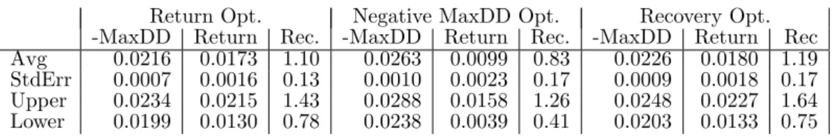
Table 5: Out-of-Sample results for EURUSD1 using three different in-sample optimization methods, 100

inde-pendent runs per method.

Return Opt. Negative MaxDD Opt. Recovery Opt.

-MaxDD Return Rec. -MaxDD Return Rec. -MaxDD Return Rec

Avg 0.0216 0.0173 1.10 0.0263 0.0099 0.83 0.0226 0.0180 1.19

StdErr 0.0007 0.0016 0.13 0.0010 0.0023 0.17 0.0009 0.0018 0.17

Upper 0.0234 0.0215 1.43 0.0288 0.0158 1.26 0.0248 0.0227 1.64

Lower 0.0199 0.0130 0.78 0.0238 0.0039 0.41 0.0203 0.0133 0.75

Table 6: Out-of-Sample results for EURUSD2 using three different in-sample optimization methods, 100

inde-pendent runs per method.

Avg 0.0374 0.0006 0.36 0.0344 0.0048 0.61 0.0263 0.0099 0.83

StdErr 0.0015 0.0028 0.10 0.0015 0.0031 0.13 0.0010 0.0023 0.17

Upper 0.0413 0.0078 0.63 0.0383 0.0128 0.96 0.0288 0.0158 1.26

Lower 0.0335 -0.0066 0.10 0.0304 -0.0032 0.27 0.0238 0.0039 0.41

bound on recovery factor, in all but one case, is also positive. This is a strong indication that the CGP method is effective.

However, the mean recovery factor is not always more than 1.0, which is desirable. For the 2006 EU-RUSD dataset, the average recovery factor is around 1.0, but it is much lower in the 2010 EURUSD dataset and the 2006 Dow Jones dataset. Surprisingly, the recovery factor is on average greater than 1.0 for the 2010 Dow Jones dataset.

The second result we will consider is the average return. Again, examining the tables, we see that while the returns are positive, they are often quite modest. For example, in the EURUSD 2006 dataset result shown in Table 5 the best return is 0.0031 or 31 points, which would only be significantly profitable if a significant investment was made (for a standard lot size of $100,000, this would amount to about $31 profit.) However, the simple negative strategy results shown in Table 4 are also quite modest at only 77 points, indicating that the market did not move far during the testing period.

Where the market did move a significant amount (for example, the Dow Jones 2010 dataset where the simple positive strategy records a $280 profit), the CGP strategies capture a significant chunk of that movement – a little over half of it with a net return of $169.35 on average.

Which of the three optimization measure is op-timal in the experiments? An examination of the results shows that for the Euro/US dollar datasets, it is optimization of recovery factor that leads to the best on-average cumulative returns (those being 0.0180 and 0.099 for the 2006 and 2010 datasets re-spectively). For the Dow Jones datasets, optimizing negative maximum drawdown leads to the best cu-mulative returns.

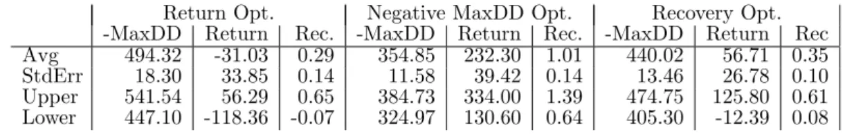
Interestingly, in none of the four experimental datasets does direct optimization for in-sample return lead to the best out-of-sample return. Additionally, optimization for return is the only strategy that leads to a negative out-of-sample return, that being $-31.03 for the 2006 Dow Jones dataset. The lesson to be learned here seems to be that it is better to optimize for minimal drawdowns than it is to optimize directly for maximum return.

4.2 Analysis of Programs

In addition to the performance of CGP-based pro-grams as trading strategies, we were also interested in the composition of the programs that were evolved. Figure 1 gives one specific example of a program that was evolved. To perform a more general anal-ysis, we examined, for each of four datasets, the 100 best-of-run programs that were tested out-of-sample. Our analysis primarily concerned the frequency with which individual functions appeared in these pro-grams. These frequencies are given in Table 9.

An examination of this table shows that that by far the most frequently selected operator is the sub-traction−operator, followed closely the comparison

<and>operators, and then theM EAN andM IN

operators. These are indeed the type of operators that one would expect to see if designing an indicator-based trading system. Interestingly, functions repre-senting constant outputs (C1,C−1, andC0) are used

very infrequently.

We also computed the average size of each best-of-run program for all four of the datasets. Those averages, in terms of the number of active nodes, are 6.16 and 6.21 for the EURUSD datasets and 4.58 and 5.34 for the INDU datasets. This shows that whereas programs of length up to 30 could have evolved, that many functions were not required and that the result-ing programs were actually reasonably simple.

5 Conclusion

To conclude, an investigation of Cartesian Genetic Programming (CGP) with different objective func-tions for the purpose of learning trading strategies has been undertaken. CGP has been shown to be ef-fective at learning strategies that often make a mod-est but significant net positive returns on data from two different markets and two different time periods. Furthermore, the method produces rules that are rel-atively simple, containing on average 5-6 functions per rule.

References

Barbosa R., Belo O. (2008)Autonomous Forex Trad-ing Agents, inProc. 2008 International Conference

(6)

Table 7: Out-of-Sample results for INDU1using three different in-sample optimization methods, 100

indepen-dent runs per method.

Avg 494.32 -31.03 0.29 354.85 232.30 1.01 440.02 56.71 0.35

StdErr 18.30 33.85 0.14 11.58 39.42 0.14 13.46 26.78 0.10

Upper 541.54 56.29 0.65 384.73 334.00 1.39 474.75 125.80 0.61

Lower 447.10 -118.36 -0.07 324.97 130.60 0.64 405.30 -12.39 0.08

Table 8: Out-of-Sample results for INDU2using three different in-sample optimization methods, 100

indepen-dent runs per method.

Avg 148.49 118.63 1.18 142.37 169.35 1.59 146.27 140.30 1.36

StdErr 5.55 13.68 0.14 4.32 11.09 0.21 5.67 14.03 0.16

Upper 162.80 153.92 1.55 153.52 197.95 2.14 160.89 176.49 1.76

Lower 134.18 83.34 0.81 131.22 140.74 1.04 131.66 104.11 0.96

on Data Mining, ICDM 2008, P. Perner Ed., LNAI 5077, pp. 389-403.

Beechey M., Gruen D., Vickrey J. (2000). The Effi-cient Markets Hypothesis: A Survey. Reserve Bank of Australia.

Contreras I., Hidalgo J., Nunez-Letamendia L. (2012), A GA combining technical and fundamental analysis for trading the stock marking. In EvoAp-plications 2012, Springer, pp.. 174-183.

Fama, E. (1970), Efficient Capital Markets: A Re-view of Theory and Empirical Work. Journal of Finance 25 (2): 383417. doi:10.2307/2325486. JS-TOR 2325486.

Hirabayashi A., Aranha C., Iba H. (2009), Optimiza-tion of the Trading Rule in Foreign Exchange using Genetic Algorithm, inProc. GECCO’09, pp. 1529-1536.

Larkin F. and Ryan C. (2010), Modesty is the Best Policy: Automatic Discovery of Viable Forecasting Goals in Financial Data. InProc. EvoApplications 2010, Part II, pp. 202-211.

Lean Y., Lai K. (2007),Foreign Exchange Rate Fore-casting with Artificial Neural Networks. Springer-Verlag.

Liu Z., Xiu D. (2009), An automated trading system with multi-indicator fusion based on D-S evidence theory in forex market, inProc. Sixth International Conference on Fuzzy Systems and Knowledge Dis-covery, IEEE, pp. 239-243.

Miller J., ed. (2011), Cartesian Genetic Program-ming. Springer.

Ni H., Yin H. (2009), Exchange rate prediction us-ing hybrid neural networks and tradus-ing indicators, Neurocomputing72:2815-2832.

Sekanina L., Harding S., Banzhaf W., Kowaliw T. (2011), Image Processing and CGP. In Miller (2011), pp. 181-216.

Sekanina L., Walker J, Kaufmann P, Platzner M. (2011), Evolution of Electronic Circuits. In Miller (2011), pp. 125-180.

Sewell, M. (2011), Characterization of Financial Time Series. Research Note RN/11/01, Dept. of Computer Science UCL.

(7)

Table 9: Percentage probability of a function being selected for a node in a best-of-run individual by dataset, over 100 independent runs per dataset.

Function EURUSD1 EURUSD2 INDU1 INDU2

+ 6.15% 4.94% 9.29% 6.31% − 15.05% 10.37% 15.55% 11.87% × 8.58% 7.97% 6.91% 7.61% / 11.33% 8.13% 8.86% 11.50% > 11.97% 16.91% 12.96% 11.32% < 12.30% 13.24% 12.53% 12.80% M AX 10.36% 9.89% 5.40% 8.16% M IN 8.25% 12.92% 8.86% 14.66% M EAN 12.14% 7.97% 13.61% 10.39% C1 1.46% 1.91% 2.38% 2.97% C−1 1.29% 2.71% 1.94% 1.30% C0 1.13% 3.03% 1.73% 1.11%

Figure 1: An example of a program evolved using CGP. Function node 17 is the output node. Each function call has two inputs. Inputs may be input data (denoted byi0,i1, etc) or the output of another function node

(denoted by an integer identifying the node). In the array representation in figure (a), active nodes are marked by marked by *. Figure (b) is the corresponding evaluation graph.

Node F Inputs Node F Inputs Node F Inputs

0* + i5,i6 10 − 6,i1 20 M AX i4,i7 1* − i7,0 11 M IN 2,6 21 × 3,5 2* M AX i2,i6 12* / 1,i1 22 M IN i3,10 3 + i7,0 13 − 10,10 23 M EAN 4,3 4 C1 i5,i4 14 M AX 5,i6 24 M EAN 3,i5 5 × i5,2 15* + i5,9 25 < 8,15 6 M AX 0,4 16 / i1,2 26 × 0,4 7 × i7,0 17* / 15,12 27 > i1,24 8 C1 1,2 18 M EAN i3,11 28 + 8,11 9* M IN i5,2 19 > 8,3 29 + 4,2 i5 ! ! D D D D D D D D D $ $ % % i6 IIII$$ I I I I I I i2 y y tttttt tttt i7 ! ! D D D D D D D D D + M AX − $ $ I I I I I I I I I I I i1 y y tttttt tttttt M IN / + /// //Output