Transactions
[email protected] ISSN: 1696-2281
eISSN: 2013-8830 www.idescat.cat/sort/
On the interpretation of differences between
groups for compositional data
Josep-Antoni Mart´ın-Fern´andez∗,1, Josep Daunis-i-Estadella1 and Gl`oria Mateu-Figueras1
Abstract
Social polices are designed using information collected in surveys; such as the Catalan Time Use survey. Accurate comparisons of time use data among population groups are commonly analysed using statistical methods. The total daily time expended on different activities by a single person is equal to 24 hours. Because this type of data are compositional, its sample space has particular properties that statistical methods should respect. The critical points required to interpret differences between groups are provided and described in terms of log-ratio methods. These techniques facilitate the interpretation of the relative differences detected in multivariate and univariate analysis.
MSC: 62F40, 62H15, 62H99, 62J10, 62J15, 62P25
Keywords: Log-ratio transformations, MANOVA, perturbation, simplex, subcomposition.
1. Introduction
Statistical offices around the world (e.g., Eurostat) state that “a time use survey measures the amount of time people spend doing various activities, such as paid work, household and family care, personal care, voluntary work, social life, travel, and leisure activities”. This type of survey offers exhaustive information concerning the social habits and the everyday life of the population. The time use data are compiled by factors such as, among others, sex, age group, household composition, level of education, professional status, and day of the week. In consequence, the analysis of time use data across the groups defined by these factors is of crucial importance because it supports the
de-∗Address for correspondence:Dept. Computer Science, Applied Mathematics and Statistics, University of Girona, Campus Montilivi (P4), E-17071 Girona, Spain, [email protected]
1Department of Computer Science, Applied Mathematics and Statistics, University of Girona, Spain. Received: October 2014
velopment of family and gender equality policies. When one has a preliminary look at time use data, one states that they arecloseddata (Aitchison, 1986). That is, the total daily time expended on different activities by anyone one person is always equal to 24 hours. In addition, the units (hours or minutes) are not relevant when one describes the time spent on one activity. The interest then, is on the proportion of time, that is, the part of the day that people do an activity. According to Aitchison (1986), time use data is one example ofcompositional data.
Compositional data (CoDa) are quantitative descriptions of the parts or components of a whole, conveying exclusively relative information. Typical examples of composi-tions appear in geochemistry, environmetrics, chemometrics, budget expenses and data from time use surveys. In this latter case, the compositions areclosed. On the other hand, if one were to analyse the solid waste composition in a household the CoDa would not be closed because the kilograms of waste vary between the families. In such cases, for con-venience, compositions are commonly expressed in terms of proportions, percentages or parts per million (ppm) and to do this theclosureoperation is applied (Aitchison, 1986). When an analyst decides to analyse a data set X (n×D) using compositional methods, he or she is assuming that the information collected is relative rather than absolute. In this sense, it holds that the information collected in any observationxis the same as in αx, for any scalar α>0, property known asscale invariance (Aitchison, 1986). However, in some cases the closure operation may be useful when the analyst is interested in the interpretation of some univariate statistics, such as percentiles. As the ratios rather than the absolute values are of interest, any function used to measure the difference between two compositions should be expressed in terms of ratios between variables. Indeed, letx1andx2 be two compositions, the vector of ratios(x11
x21, . . . , x1D x2D)
should play an important role when one interprets the difference between x1 and x2 (Aitchison and Ng, 2005). These ideas for dealing with CoDa were introduced in the early 1980s, when the use of logratios was proposed by Aitchison (1986). At the beginning of the current century, the use of orthonormal log-ratio coordinates was introduced in Egozcue et al. (2003). The critical concept of these approaches is that compositions have a natural geometry, known as the Aitchison geometry (Egozcue and Pawlowsky-Glahn, 2006), which is coherent with the relative scale of compositions.
Our interest is to compare the use of time between groups of people defined by factors such as professional status, level of education or municipality size. When one compares groups of data, descriptive techniques, models and the corresponding infer-ential techniques are commonly used. All of these elements have to be appropriate for the type of data collected. For example, some models consider that random multivariate observationsX from a group are generated byadding a random variation or noise ε
around a fixed centreµ. Although the typical modelX=µ+εcan be appropriate for interval scale data, this model would not be useful for ratio scale data such as CoDa. For example, in the case of data from a time use survey, when the centreµtakes a small value for some activity, the resulting compositionx may take negative values. More-over, most common parametric and non-parametric methods for analysing differences
between groups deal withvariability matrices: total, between and within. The critical idea is how to compare the variabilityinsidethe groups with the variabilitybetweenthe groups. For interval scale data these variabilities are measured using the typicalsum of squaresmatrices. However, for CoDa these elements should be appropriately defined in terms of ratios (Aitchison, 1986). Multivariate analysis of variance (MANOVA) is the conventional name for the contrast of the equality of means in several groups (Wilks, 1932; Smith et al., 1962). MANOVA and its related parametric methods include infer-ential techniques based on the multivariate normal distribution. The approach known as theprinciple of working on log-ratio coordinates(Mateu-Figueras et al., 2011) sug-gested the definition of the normal distribution for CoDa (Mateu-Figueras et al., 2013). With these elements at hand, the MANOVA contrast can be coherently defined to the particular geometry of CoDa.
The main objective of this article is to provide the critical points required to inter-pret differences between groups for CoDa. In Section 2, some descriptive statistics and techniques for CoDa are presented. Section 3 provides the complete proposal of a com-positional MANOVA contrast. The interpretation of multiple comparisons and related techniques are also described. The example that motivated this article is presented in Section 4, where all the elements introduced for interpreting differences are applied. Fi-nally, in Section 5, some concluding remarks are provided. The programming of the data analyses discussed in this article was carried out using the open source R statistical pro-gramming language and software (R development core team, 2014) and the freeware Co-DaPack (Comas-Cuf´ı and Thi´o-Henestrosa, 2011). The computer routines implementing the methods can be obtained from the websitehttp://www.compositionaldata.comand the R-package “zCompositions” (Palarea-Albaladejo and Mart´ın-Fern´andez, 2014).
2. Compositional descriptive techniques
2.1. Logratio coordinatesAccording to the ratio scale nature of CoDa, any function f(·)applied to a composition xmust verify that f(x) = f(αx),for anyα>0. In particular,
f(x) = f(x1,x2, . . . ,xD) = f xk x1 xk , . . . ,x(k−1) xk ,1,x(k+1) xk , . . . ,xD xk = = f x1 xk , . . . ,x(k−1) xk ,x(k+1) xk , . . . ,xD xk , fork=1, . . . ,D.
In other words, any function should be expressed in terms of ratios between variables. Note that any ratio xj/xk is not symmetric and takes values in (0,+∞). However, a
the zero origin. Following Aitchison (1986), the general expression of a logratio is a log-contrast a1ln(x1) +. . .+aDln(xD) =ln D
∏
j=1 xajj ! , (1)where∑aj=0, so as to verify the scale invariance property. A log-contrast is, in essence,
a logratio of parts because foraj>0 the corresponding partxjappears in the numerator,
but ifaj<0 it appears in the denominator, and for those parts that do no contribute to
the logratio, thenaj=0 holds. Importantly, log-contrast (1) has the same role as linear
combinations of variables in classic statistics. Note that ratios and logratios can not be calculated when one of the parts takes the value zero. The treatment of this difficulty, also known as thezero problem, has recently been described in numerous articles. A reader interested in this topic will find a general description in Palarea-Albaladejo et al. (2014).
Using a log-contrast one can define new variables (e.g., latent variables or principal components) where the information collected in the original variables is combined. One example of the very useful new variables is thecentred log-ratio(clr) defined in Aitchison (1986) by clr(x)k=ln xk
(∏xj)1/D =lnxk−ln
x, k=1, . . . ,D. The log-contrast expression (1) of a clr-variable verifies thatak j =−1/Dfor j=6 kandakk=1−1/D.
The clr variables, also known as clr coordinates, have another interesting interpretation: they are the log-coordinates centred by rows. Therefore, it holds that∑Dk=1clr(x)k=0, indicating that the dimension of the clr coordinates’ space isD−1. The critical element of the Aitchison geometry is the scalar product defined via the log-ratio coordinates. Indeed, letx1andx2be two compositions, then<x1,x2>a=<clr(x1),clr(x2)>e. Here the subscriptsaanderepresents respectively Aitchison and Euclidean metric elements. As usual, one can derive a distance and norm from the scalar product and finally obtain
da(x1,x2) =de(clr(x1),clr(x2)), and ||x1||a =||clr(x1)||e. Remarkably, the Aitchison
distance verifies that da(x1,x2) = ||(xx1121, . . . ,xx12DD)||a, providing information about the
relative difference between two compositions.
These metric elements are used to construct orthonormal basis and calculate the corresponding orthonormal log-ratio coordinates (Egozcue et al., 2003). The expression of these coordinates, known as isometric log-ratio coordinates (ilr), depends on the basis selected. Following Egozcue and Pawlowsky-Glahn (2005) one can define a particular ilr coordinates created through a sequential binary partition (SPB). According to equation (1), to make any logratio consists of selecting which parts contribute to the logratio and decide if these will appear in the numerator or in the denominator. In the first step of an SBP, when the first ilr coordinate is created, the complete composition x= (x1, . . . ,xD) is split into two groups of parts: one for the numerator and the other for the denominator. In the following steps, to create the following ilr coordinates, each group is in turn split into two groups. That is, in stepk when the ilr(x)k coordinate
is created, the r parts (xn1, . . . ,xnr) in the first group are coded as +1 and placed in
the numerator, and the s parts (xd1, . . . ,xds) in the second group will appear in the
denominator and coded as -1. As a result, the ilr(x)kis
ilr(x)k= r rksk rk+sk ln(xn1· · ·xnr) 1/rk (xd1· · ·xds)1/sk ,k=1, . . . ,D−1. (2) whereq rksk
rk+sk is the factor for normalizing the coordinate. The log-contrast expression
(1) of a ilr-variable verifies thatak j=
q s
k
rk(rk+sk)if the partxjis placed in the numerator,
andak j=−
q r
k
sk(rk+sk) for parts that appear in the denominator.
The metric elements can be also expressed in terms of ilr coordinates (e.g.,da(x1,x2) =
de(ilr(x1),ilr(x2))) as these coordinates are equal to the clr coordinates expressed on an
orthonormal basis (Egozcue et al., 2003). The most important point here is that, once an orthonormal basis has been chosen, all standard statistical methods can be applied to the log-ratio coordinates and transferred to the simplex preserving their properties (Mateu-Figueras et al., 2011). The log-ratio approach proposed by Aitchison (1986) and the proposal to work on log-ratio coordinates do not differ substantially. In fact, the only distinction is the recommended use of orthonormal (or ilr) coordinates in the latter ap-proach instead of the use of clr transformed vectors (see Mateu-Figueras et al. (2011) for an in-depth discussion). Note that, when a statistical method is applied to the ilr coordi-nates, one must analyse whether the results depend on the particular orthonormal basis selected. In other words, one must assure oneself that the interpretations are invariant un-der changes of basis. In this scenario, the advantage of the ilr coordinates created by an SBP is the interpretation of results and the corresponding CoDa-dendrogram, described in the following section.
2.2. Descriptive statistics and plots
Most of the multivariate methods for dealing with groups are based on location and spread (shape) descriptive statistics. In this paper we focus on the common centre and variability elements, accordingly modified to take into account the Aitchison geometry. Let X be a random composition. In practical terms, Pawlowsky-Glahn and Egozcue (2001) stated that the centre µ is the geometric mean of X, whose ilr coordinates ilr(µ) are, respectively, equal to the arithmetic mean of ilr(X). The covariance of X is cova[X] =Σ=cov[ilr(X)]. In consequence, a comparison ofg groups with respect
to its location will be based on the comparison between the correspondingg centres
µj, j=1, . . . ,g. Indeed, for a data set withncompositions distributed inggroups, we
can use the matrices total (T), between-groups (B), and within-groups sums of squares matrices (W). These matrices verify the variability decomposition property:T=B+W. Animportantcontribution of matrixBin this equality suggests that there are relevant
differences between the groups with respect to its location. The approach used for evaluating thisimportancemeans techniques differ from one another. In this article we focus on the MANOVA contrast that evaluates this contribution using measures based on the trace, determinant and eigenvalues of these matrices. To compare the spread of the groups, for example to evaluate the homoscedasticity, one will compare the within-groups sum of squares matrices. Besides the location case, there are few techniques for evaluating differences with respect to the variability.
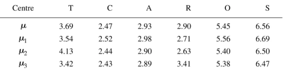
For example, we considered that a first group is the data set statistician’s time budget(Aitchison, 1986) formed by 20 compositions with six parts (T,C,A,R,O,S), corresponding to time spent on daily activities: Teaching, Consulting, Administration, Research, Other, and Sleep. Next, we generated a second group perturbing the 20 samples multiplying them component-wise by the vector (1.2,1,1,1,1,1), that is, increasing by 20% the first activity ratio against the other activities. Finally, we created a third group perturbing the initial 20 samples by the vector(1,1,1,1.3,1,1)to increase by 30% the fourth component ratio against the other components. Hereinafter, we refer to the whole CoDa set as theST3data set. Note that the three groups have the same covariance matrix because the second and third groups were created by perturbing the first group (Aitchison, 1986). Table 1 shows the unitary representative of the centre (µ) of the whole ST3 data set and the centres (µj, j=1,2,3) of the three groups. As expected, the larger differences occur in partsT andR.
Table 1: Centres in ST3: for the whole data set (µ) and for the three groups (µj).
Centre T C A R O S
µ 3.69 2.47 2.93 2.90 5.45 6.56
µ1 3.54 2.52 2.98 2.71 5.56 6.69
µ2 4.13 2.44 2.90 2.63 5.40 6.50
µ3 3.42 2.43 2.89 3.41 5.38 6.47
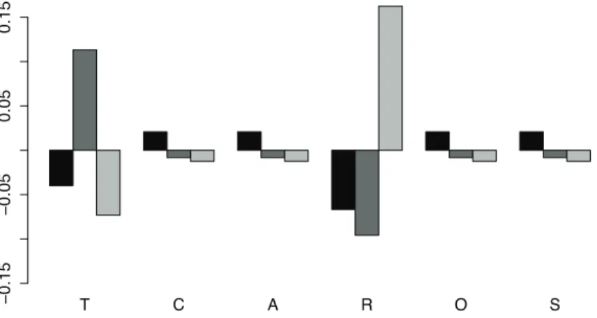
The geometric mean barplot (Figure 1) is an option for describing differences between groups. Given a CoDa set, for each group, the logratio between the whole geometric mean and the geometric mean of the group is calculated. Finally, each component is represented in a barplot using a logarithmic scale. If the centre of the group is equal to the whole centre, the ratio of each component is one and the corresponding logarithm is zero. If one part of the centre of the group is greater or smaller than the corresponding part of the whole centre, then the ratio is different than one and the corresponding logarithm is respectively positive or negative. Indeed, large bars (positive or negative) will indicate large differences in the means. Figure 1 shows that in the partsC,A,O, andS, the differences between the groups and the whole data set are not relevant. The samples from the second group have large values in partT, whereas they take small values in the rest of the parts. A similar situation occurs in the third group
Figure 1: Geometric mean barplot for ST3 data set: first group (black), second group (dark gray), third group (light gray).
with respect to partR. Note that, for example, when a bar in one part is larger than 0.15, one can interpret that, on average, the samples of this group are in this part 16.18% (exp(0.15) =1.1618) larger than the whole centre.
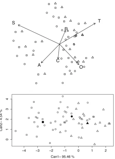
To complete the basic description of a grouped CoDa set, one can represent the data using three specific plots: a biplot, a canonical variates plot and a coda-dendrogram. Aitchison and Greenacre (2002) adapted the typical biplot for CoDa and in doing so introduced the clr-biplot, that is, the biplot of clr coordinates. In other words, a clr-biplot draws on the same plot a projection of scores in the first two clr principal components together with the centred clr variables. Daunis-i-Estadella et al. (2011) described the interpretation of clr-biplots and introduced an extension for including supplementary elements. However, the statistical technique that underlies a biplot is not specially designed for highlighting differences between groups. In some cases, despite the groups being different, they appear mixed in the biplot. Figure 2(up) shows the clr-biplot of the ST3 data set. This representation is of a medium quality because the two first axes retain 61% of the variability. The samples of the first group are represented by circles. The compositions of the second group are shown by the triangles and shifted slightly to the positive part of the clr variable associated to the partT. On the other hand, as expected, the squares representing the third group are shifted to the positive direction of the clr-transformed partR. However, the samples from the different groups appear mixed, suggesting that there are no relevant differences between the groups.
As an alternative to the biplot, one can consider the canonical variates plot. Broadly speaking, a canonical variate is a new variable obtained as a linear combination of the original variables, where the linear combination attemps to highlight any differences between theg groups. For CoDa, we will use log-contrasts to create these new vari-ables. Indeed, using ilr coordinates, a canonical variate y is equal to y=vTilr(x) =
∑Dj=−k1vkilr(x)k, that is, y is also a log-contrast. According to the general procedure, the
Figure 2: Compositional plots for ST3 data set: clr-biplot (up) and canonical variates plot of ilr coordi-nates (down). Samples of the three groups are respectively represented by circles, triangles and squares.
associated with the ANOVA test:H0:vT1µ1=. . .=vT1µg It could be proved that the
vector v1 is the eigenvector of matrix W−1B associated to its maximum eigenvalue. Following this procedure iteratively, we can obtain the ordered D−1 eigenvectors that define the corresponding canonical variates. Importantly, if a change of basis is applied and the new ilr coordinates are Ailr(x), with A an unitary matrix (ATA= I), then taking A v, the same canonical covariate is obtained. In other words, the invariance under change of basis is guaranteed. Figure 2(down) shows the two first canonical variates plot for the ST3 data set. In addition, the centres of each group are represented by a filled symbol. The samples from different groups appear well separated, suggesting that there are relevant differences between the groups. In this case, the first eigenvector of matrixW−1Bisv1= (3.75,−0.37,10.31,3.57,0.31)Twhich, combined with the coefficients of log-contrast in equation (2), produces the first canonical variate
log-contrast with coefficientsa= (6.33,1.03,4.13,−8.08,−3.13,−0.28)T. To perturb only the first part of the samples of the first group by 1.2 is equivalent to adding 6.33 ln(1.2) =1.15 to the first canonical variate. The perturbation of the fourth part by 1.3 is equivalent to adding−8.08 ln(1.3) =−2.12 to the scores in the first canonical variate.
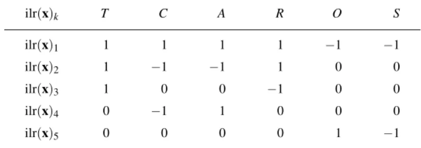
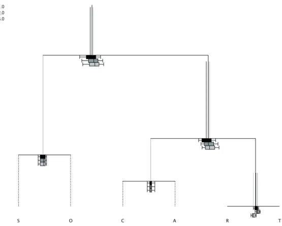
A CoDa-dendrogram is a descriptive plot for visualizing some univariate statistics of particular ilr coordinates created through a SPB (Pawlowsky-Glahn and Egozcue, 2011). Table 2 shows the complete SBP for the ST3 data set.
Table 2: Sequential Binary Partition for ST3 CoDa set.
ilr(x)k T C A R O S ilr(x)1 1 1 1 1 −1 −1 ilr(x)2 1 −1 −1 1 0 0 ilr(x)3 1 0 0 −1 0 0 ilr(x)4 0 −1 1 0 0 0 ilr(x)5 0 0 0 0 1 −1
The SBP is represented by the dendrogram-type links between parts (Figure 3). The variability of each ilr coordinate is represented by the length of the vertical bars. Therefore, a short vertical bar, as in the case of ilr(x)3 and ilr(x)4 means that the ilr coordinate has a small variance. Conversely, when the ilr coordinate has a large variance its vertical bar is longer, as in ilr(x)2 which involves the parts T and R. The location of the mean of an ilr coordinate is determined by the intersection of the horizontal segment with the vertical segment (variance). When these intersections are not in the middle, this indicates a major contribution of one of the groups of parts. This is the case of ilr(x)1, where the intersection is close to partsOandS, according to its larger values (Table 1) with respect to the values in the other parts. In addition, the box-plot of the ilr coordinates is provided. Note that for the coordinate ilr(x)3, the box-plots are ordered according to the perturbation applied to create the corresponding group. One can analyse its symmetry and compare the median with the mean to interpret the symmetry of the corresponding univariate distribution. Figure 3 shows these statistics of the ilr coordinates for the three groups in ST3 data set. Note that there are no differences between the variances between the groups but there are differences between the means in the coordinates ilr(x)1, ilr(x)2, and ilr(x)3. For the coordinate ilr(x)3there is a difference between the mean of first group (black colour) and the mean of second group (dark gray colour) and third group (light gray colour). This fact is consistent because ilr(x)3 evaluates the ratio between the partsT andR. The second group mean is close to partT
and the mean of third group is close toR. This interpretation agrees with the construction of these groups by perturbing the first group.
Figure 3: CoDa-dendrogram for ST3 data set using the SBP from Table 2. Elements of three groups 1, 2, and 3 are distinguish by the colours black, dark gray and light gray, respectively.
3. Inferential techniques to compare CoDa groups
3.1. MANOVA contrast for CoDaIn the statistical literature there are many inferential methods for comparing groups of data in the real space. Following Aitchison and Ng (2005), in this article we focus on the most basic methods to show how to proceed when one wants to be coherent with the Aitchison geometry. Other more sophisticated methods could be adapted accordingly to the compositional geometry by using an analogous procedure.
Let Xk be a random composition corresponding to the group k for k =1, . . . ,g. The more basic model assumes that Xk is generated adding a random variability εk around a centreµk in a multiplicative part-wise way: Xk=µ
k⊙εk. In this case, the
expected value of variabilityεkis the unit vector1. Following Egozcue et al. (2003) and
according to the principle of working on coordinates (Mateu-Figueras et al., 2011), this model is equivalent to ilr(Xk) =ilr(µk) +ilr(εk), where ilr(εk)is centred at the origin of
as for interval scale data in the real space. From the different approaches for dealing with this type of model, in this article we focus on the MANOVA contrast (Wilks, 1932; Smith et al., 1962) and related techniques. The technical details of these methods are provided by the majority of books devoted to multivariate statistical techniques (e.g., Seber, 1984).
The critical assumption of the MANOVA contrast is that the ilr random variability ilr(εk)is homocedastic and normally distributed, that is, ilr(εk)∼N (0,Σ);k=1, . . . ,g.
Following Mateu-Figueras et al. (2013), this assumption is equivalent to assuming log-ratio normality and homocedasticity for the compositional termεk. In addition, the
orig-inal null hypothesisH0:µ1=. . .=µgis equivalent to the null hypothesisH0: ilr(µ1) =
. . .=ilr(µg). Therefore, the statistics of contrast will be based on the sum of square ma-tricesT,B, and Wcalculated on ilr coordinates. The most common contrast statistics are: Wilks’Λ(det(W)/det(T)), Pillai’s trace (trace(B T−1))), Lawley-Hotelling trace (trace(W−1B)), and Roy’s largest root of matrixW−1B. Nowadays, the discussion over the merits of each statistic continues and the common software routines allow the four statistics to be calculated. In the case of two groups, the four statistics are equivalent and the MANOVA contrast reduces to Hotelling’s T-square test. Importantly, the MANOVA contrast is invariant under a change of log-ratio basis because the four statistics are in-variant functions of the eigenvalues of matrixW−1B. This fact facilitates the use of the contrast because one can work with the ilr coordinates obtained from an SBP.
When the assumptions are accomplished the four statistics are associated to a value in anF probability distribution, permitting the calculation of a p-value for the MANOVA contrast. The first assumption, the homogeneity of variances and covariances (H0:Σ1=. . .=Σg), can be tested using the Box M test (Seber, 1984, p. 449). This test
has been severely criticized because it is very sensitive to lack of normality, so that a significant value could indicate either unequal covariance matrices or non-normality or both. The general recommendation is to take a significant level less than 0.005. Nevertheless, if the number of subjects in each of the groups are approximately equal, the robustness of the MANOVA test is guaranteed and the impact, if the assumption of equal covariances is violated, is minimal (Johnson and Wichern, 2007). Noticeably, because Box M statistic is a function of the covariance matrices determinant, it could be proved that the results of the Box M test are invariant under changes of basis. Moreover, the equality of covariances can be descriptively checked using the CoDa-dendrogram. Because the vertical lines in the plot (Figure 3) represent the variance of each ilr coordinate, then we can evaluate if there are differences in the variances of each group. Figure 3 suggests that the variances of each ilr coordinate are equal because the three lines are of similar length. However, a CoDa-dendrogram only allows the variances of ilr coordinates to be compared, that is the diagonal of matrices Σk. Despite being
unusual, it could be that the random compositionsXkhave equal variances but different covariances. That is, the matricesΣk have equal diagonals but the rest of elements are
different. To investigate this case we propose to previously sphericize the data to plot the CoDa-dendrogram. A spherification, similar to the standardization in the univariate
case, consists of multiplying the residuals ilr(εk) of each group by the squared root of
W−1, the inverse of covariance matrix. After this transformation, if the homocedasticity is verified, the resulting covariances matrices in each group should be the identity matrix. In consequence, in the CoDa-dendrogram of spherized data, the vertical lines of all the groups for all the ilr coordinates should be equal.
The second assumption for the MANOVA contrast is the normality of the residuals
εk. One can apply to the their ilr coordinates any of the multivariate normality tests
that exist in the literature. For example, we can use the goodness-of-fit test suggested in Aitchison (1986) for compositional data. This test is based on the idea that, under the assumption of normality, theradii(or squared Mahalanobis distances) of the residuals are approximately distributed as a chi-squared distribution. We can use some empirical distribution function statistics, for instance Anderson-Darling or Cramer-von Mises, to test significant departures from the chi-squared distribution. Importantly, because Mahalanobis distances are invariant under change of basis, this normality test can be calculated using any ilr coordinates obtained with an SBP. To complete the analysis of this assumption, the normality can be explored using a typical Q-Q plot of the radii against the theoretical quantiles of a chi-squared distribution. Finally, according to Johnson and Wichern (2007), the assumption of normality in a MANOVA contrast can be relaxed when the sample sizes are large due to the multivariate version of the central limit theorem.
3.2. Analysing differences between groups
When MANOVA contrast or another test suggest rejecting the null hypothesis of equality of means, two questions immediately arise: (a) Which groups differ from the rest and (b) which variables are responsible of these differences? One common way to investigate the answer of these questions is by making the corresponding
g(g−1)/2 comparisons between pairs of groups. Following the MANOVA approach, these comparisons can be analysed through the Hotelling’s T-squared test, which is the multivariate generalization of a typicalt-test. In this procedure, there is a general recommendation to avoid an artificial increase of the Type I Error rate: to adjust the alpha level of each test by making some kind of correction. Although there is no general agreement about the way to make this correction, a common technique is the Bonferroni correction for simultaneous tests (Seber, 1984). Following this technique one should modify the critical level α to α/(g(g−1)/2). However, this procedure tends to be conservative, especially when the number of comparisons is large. There are other more sophisticated procedures, such as the Scheffe’s, the Tukey’s or the Student-Newman-Keuls tests or another different approach provided by the FDR False Discovery Rate controlling method (Benjamini and Hochberg, 1995; Benjamini, 2010). The techniques for dealing with multiple comparisons are currently an open field whose development is beyond the scope of this article.
Regardless of this analysis, note that when using Hotteling’s T-squared test on ilr coordinates the invariance under change of basis is guaranteed. In addition, these differences can be explored using the canonical variates plot, where one may also draw the corresponding confidence region for the mean and the predictive region for each group. With this plot one has a complete picture of the differences between groups, analysing if the corresponding regions overlap or not.
Once differences between two particular groups are detected, interest focuses on discovering if there are ilr coordinates responsible for these differences. That is, if the differences stated using multivariate techniques may be attributed to any separate variable. Following the previous approach, these univariate comparisons will be done through D−1 simultaneous t-tests. Again, in this case it is accordingly necessary to adjust the critical level or use a more complex technique. Remarkably, the results of these comparisons strongly depend on the ilr coordinates selected because one is making univariate t-test for a particular orthonormal basis. As a consequence, the choice of an interpretable SBP turns out to be crucial. For this analysis, the geometric mean barplot may be very useful for completing the interpretation of the univariate log-ratio differences because this plot allows all the parts to be compared directly. In addition, following Hesterberg et al. (2012), one can add the uncertainty associated to the geometric mean barplot using a bootstrap technique for comparing two populations. LetX1andX2be two groups withn1andn2compositions, respectively:
1. Draw a resample of sizen1with a replacement from the first group and a separate
resample of sizen2from the second group. Compute the centre of each group and
calculate its log-ratio part-wise vector.
2. Repeat this resampling processBtimes (commonBis 1000).
3. Construct the bootstrap confidence interval for each part of the log-ratio vector. Note that the critical level of confidence intervals should be appropriately corrected. There are four common types of bootstrap confidence intervals: t, percentile, bias-corrected, and tilting. The description of their properties is provided by Hesterberg et al. (2012). For example, to calculate theα% bootstrap percentile confidence interval, one should calculate the interval between theα/2th and(1−α/2)th percentiles of the bootstrap distribution of the corresponding part in the log-ratio vector. Regardless of which type of interval is calculated, if the interval for a part includes the value zero, it indicates that there is no difference between these groups with respect to this part. Only the parts with positive or negative intervals may be considered as responsible for the difference between the groups.
For the ST3 CoDa set we obtained p-values below 0.001 for the four statistics in the MANOVA contrast, indicating to us to reject the null hypothesis of equality of means. The radii normality tests based on the Anderson-Darling, on the Cramer von-Mises, and on the Watson statistic show p-values above 0.15, suggesting that the normal
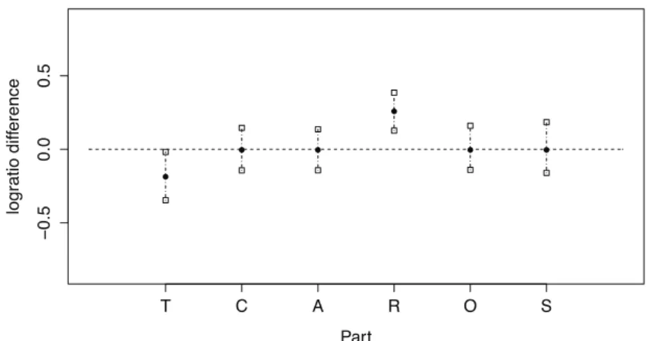
Figure 4: Bootstrap percentile confidence intervals for log-ratio difference between centres of second and third group in CoDa set ST3. Filled circles are the log-ratio difference for the centres in ST3. Vertical dashed lines are the percentile intervals.
probability distribution fits the data well. In this case, the Box M test is not necessary because by construction the three groups have the same covariance matrix. Figure 2(down) suggests that there are differences between the three groups, later confirmed by the three HotellingT-squared simultaneous tests (p-value<0.05/((3×2)/2) =0.0167, Bonferroni correction). According to the construction of groups, the SBP in Table 2 suggests that the groups are equal in ilr(x)4and ilr(x)5. They could only have relevant differences in the three first ilr coordinates. When the univariate ilr coordinates are analysed through simultaneoust-test, only ilr(x)3confirms the differences between the three groups because the larger p-value, obtained when comparing 1 and 2, was lower than the corrected alpha level (p-value=0.0034<0.0167/4= 0.0042, Bonferroni correction). These differences are associated to large values in activitiesT orR, or both. For example, we detected that the difference is on both parts when groups 2 and 3 were compared using the bootstrap percentile confidence intervals (B=1000). Figure 4 shows these intervals for the corresponding corrected critical value. The filled circles represent the difference between the centres in the CoDa set ST3. The dashed vertical lines are the bootstrap percentile confidence intervals, whose extremes are the corresponding percentiles. Only theT and R intervals do not have the value zero (horizontal line), indicating that the univariate differences are confirmed.
4. Example
We used a data set kindly provided by the Statistical Institute of Catalonia (Idescat) in Catalonia, Spain. It consists of information collected using a face to face survey of 6471 persons aged 10 and over. Household participants were randomly selected according to
a double stratified sampling design to guarantee that the selected sample is a reflection of the general population. The survey provides information on the main activity the individual does during each of the 144 10-minute slots, which make up a day. On a primary level, the survey considers a list of 34 different possible activities. However, to better interpret the results, Idescat’s official reports aggregate these activities into a minimum set of 5 main activities: personal care and sleep (CS), paid work and study (WS), household and family care (HF), social activities (SA), and commuting and others (CO). Moreover, the survey collected additional information related to many other aspects such as geographical area, municipality size, day of the week, household composition, sex, age, nationality or professional status. In consequence, any appropriate statistical analysis of the whole data set requires more general and complex methods. Because this type of analysis is beyond the scope of this article, we focused on a simple comparison between groups of data. In particular, to illustrate the CoDa techniques we attempted to solve the question: As regards to municipality size, are there any differences between time use composition of working people in a usual working day? Despite the fact that there are many other similar questions that might be analysed, this one is the most interesting to design regional polices. Note that, any other similar question may be analysed using an analogous procedure.
A preliminary inspection of data shows that the participant #1606 has a zero in the activity personal care and sleep. This participant is considered as an anomalous composition and it is removed accordingly from the data set. To obtain more realistic results we also removed those participants who’s sampled day was an unusual day. That is, 668 participants who, for some unforeseen reason (illness, accident, or public holiday), did not carry out their usual activities and so were not included in the analysis. According to Idescat’s reports, we considered that working days were from Monday to Thursday and working people, the participants that self-declared being in paid employment or studying. After the aforementioned steps, the sample size of the data set included in the analysis was reduced to 1051 participants. Only 253 from these compositions contain at least one zero, which represents an overall 5.2% of the values in the data set. The parts CS and WS have no zeros. The parts HF, SA and CO have respectively 18.55%, 4.28%, and 3.14% of their values equal to zero. According to the nature of these three parts, these zeros are considered as censored values consequence of the sampling design. Because of the data correspond to the main activity during a 10-minute slot, we assumed a threshold equal to 10 minutes for the censored values. These values were imputed using the log-ratio robust method based on a modified Expectation-Maximization algorithm (Palarea-Albaladejo et al., 2014; Palarea-Albaladejo and Mart´ın-Fern´andez, 2014).
As regards to the size of the municipality, Idescat classified the participants into three groups: small, medium and large. Table 3 shows the number of inhabitants that define these sizes and the number of participants of each group. Remarkably, the three groups have comparable sample sizes.
Table 3: Time Use data set: groups defined by municipality size.
Size Group numbering Inhabitants limit Participants
Small 1 <20000 369
Medium 2 [20000,100000] 311
Large 3 >100000 371
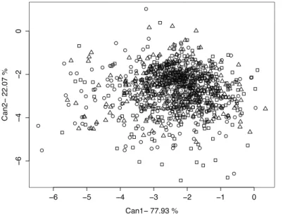
Figure 5 shows the ilr canonical variates, where the first one retains 77.93% of the variability. The participants who live in a small municipality (Group 1) are represented by circles. The triangles and squares represent participants of Groups 2 and 3, respec-tively. Participants appear mixed and no evidence of large differences between groups is detected. We used numbered circles to show the position of the geometric centre of each group. Apparently, Groups 1 and 2 have similar average values and the centre of Group 3 appears slightly separated.
Figure 5: Canonical variates plot of ilr coordinates for Time Use data set. Samples of the small (1), medium (2) and large (3) municipalities are respectively represented by circles, triangles and squares. The geometric centres of each group are accordingly represented by numbered circles.
Using equation (2) the log-contrast coefficients of the first canonical variate are a= (−0.50,−0.83,−0.28,0.34,1.27). We can interpret the slight differences between Group 3 and the other groups in terms of an opposition between the three first parts (CS, WS, HF) and the parts (SA, CO). The largest weights correspond to WS and CO parts. This interpretation is coherent with the values shown in Table 4. The largest values the SA and CO parts are taken from the group from the large municipalities. To the contrary, Groups 1 and 2 take largest values in WS part. In summary, people from large
Table 4: Centres of groups in Time Use data set: personal care and sleep (CS), paid work and study (WS), household and family care (HF), social activities (SA), and commuting and others (CO).
Group CS WS HF SA CO
1 10.97 8.72 1.15 1.89 1.28
2 10.66 8.74 1.19 2.11 1.31
3 10.80 8.50 1.02 2.13 1.55
municipalities expend more time on SA and CO, this time is subtracted to parts WS and HF.
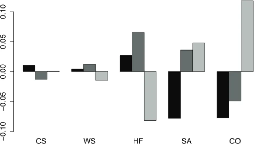
These differences are illustrated in Figure 6. When compared with the whole geo-metric centre, the largest differences appear in HF, SA and CO. On the other hand, the barplot suggests that the values in CS and WS are very similar.
Figure 6: Geometric mean barplot for Time Use data set: Group 1 (black), Group 2 (dark gray), and Group 3 (light gray).
The MANOVA contrast confirms these differences because all the p-values provided by the common contrast statistics are lower than 0.05, where the largest p-value was 0.0001969, the value for the Wilks’ Λ. When the groups were compared by pairs, the behaviour suggested in Figure 5 was confirmed. For Groups 1 and 2, the p-value was equal to 0.107. On the other hand, for Groups 1 and 3 was 0.000255 and for Groups 2 and 3, 0.003079, both lower than the Bonferroni correction level 0.05/3=
0.0166. For these cases, we investigated which log-ratio coordinate was contributing to these significant differences between groups. The alpha level was provided by the corresponding Bonferroni correction 0.05/(3×4) =0.0042. After applying the t-test to the four coordinates for the data from Groups 1 and 3, we only obtained significant differences for the fourth coordinate (p-value=0.0006). This behaviour was repeated when the data involved were from Groups 2 and 3 (p-value=0.0004). According to the equation (2), the fourth coordinate provides information about the ratio of part CO over
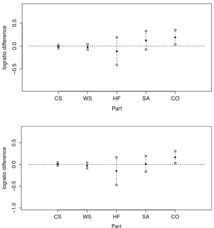
Figure 7: Time Use data set. Bootstrap percentile confidence intervals for log-ratio difference between centres of: first and third group (up); second and third group (down). Filled circles are the log-ratio difference for the corresponding centres. Vertical dashed lines are the percentile intervals.
the geometric mean of the other parts. Following this result, we investigated if the CO part was responsible of these differences. Figure 7(up) shows the bootstrap percentile confidence intervals when first and third groups are compared. The alpha level was provided by the corresponding Bonferroni correction 0.05/(3×5) =0.0033. The picture for the comparison between Groups 2 and 3 is shown in Figure 7(down). Both figures suggest the same behaviour, that is, the only significant difference appears in part CO. The percentile interval in both cases appears above the reference line. Because the log-ratio comparison uses the data from the third group in the numerator, this position means that participants in the third group take greater values than in the other two groups. In other words, people from large municipalities expend significantly more time on the Commuting and Others activities.
When the homogeneity of log-ratio variances and covariances was checked using the Box M test, we obtained a p-value equal to 0.8244. That is, we assumed that covariance matrices were not significantly different. On the other hand, when we applied theradii
Figure 8: Time Use data set. Chi-square plot of Manova contrast residuals.
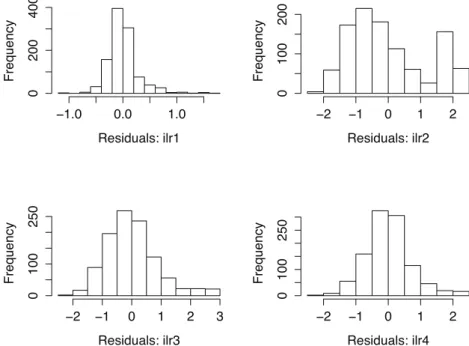
Figure 8 suggests that this lack of normality is caused by samples taking extreme values. This typical pattern is also evident in the histogram of the residuals shown in Figure 9. Despite the Gaussian shape of these histograms, the presence of extreme values may cause the lack of normality. In this case, due to our large sample size, the multivariate version of the central limit theorem guarantees the robustness of MANOVA results even the lack of normality. As indicated in Section 3.1, the non-normality could also affect the Box M test and a lower p-value could be obtained. However, this effect was not appreciated in our case because a large Box M test p-value was obtained.
5. Final remarks
Because time use data are compositional, any statistical analysis has to take into account their relative nature. This article fills the gap for basic methods for comparing groups of CoDa. We introduced descriptive techniques (log-ratio canonical variates and geometric mean barplots) for an initial exploration into the differences between groups. These differences can be confirmed by the typical inferential tools (MANOVA contrast). We introduced the bootstrap log-ratio percentiles to improve the interpretation of univariate differences and to complete the analysis of the log-ratio coordinates. Because most of these techniques are based on the principle of working on log-ratio coordinates, a detailed discussion of its invariance under change of basis was provided. The methods described assume normality and homocedasticity. When these assumptions are violated, another family of techniques should be explored, such as robust methods or distance based methods. These techniques should be applied accordingly to log-ratio coordinates to assure an appropriate analysis of the relative information collected in CoDa.
The Time Use data set provided by Idescat, is a complex data set that requires more sophisticated and general methods. However, we realised that no literature deals with these type of data using recent advances in CoDa analysis. The log-contrast approach provided in this article will be helpful to develop more complex methods, such as structural equation modelling. In addition, any general models for time use data have to include the presence of essential or structural zeros. These types of zeros represent absolute zeros, that is, it makes no sense to replace them by small values because they are not a consequence of the sampling design. The analysts should use their prior knowledge to decide what type of zero is present in a part. For example, survey participants that do not work or study have an essential zero in this part. On the other hand, in our example, after an appropriate amalgamation the zeros were considered as a consequence of sampling design. Because the greater the number of different activities are considered, the more zeros are collected, the appropriate amalgamation of parts is recommended. The development of these types of models is one of the more interesting challenges in current compositional data analysis.
Acknowledgments
This research was supported by the Ministerio de Econom´ıa y Competividad under the project “METRICS” Ref. MTM2012-33236; and by the Ag`encia de Gesti´o d’Ajuts Universitaris i de Recerca of the Generalitat de Catalunya under the project Ref: 2014SGR551. Finally, we would like to thank the Statistical Institute of Catalonia (Idescat) for kindly providing the Time Use data set.
References
Aitchison, J. (1982). The statistical analysis of compositional data (with discussion).Journal of The Royal Statistical Society Series B, 44, 139–177.
Aitchison, J. (1986).The Statistical Analysis of Compositional Data. Chapman & Hall, London 416 pp. Reprinted in 2003 by Blackburn Press.
Aitchison, J. (2001). Simplicial inference. In: M. A. G. Viana and D. S. P. Richards (Eds.),Algebraic Methods in Statistics and Probability, Volume 287 of Contemporary Mathematics Series, pp. 1–22. American Mathematical Society, Providence, Rhode Island (USA), 340 p.
Aitchison, J. and Greenacre, M. (2002). Biplots for compositional data.Journal of The Royal Statistical Society Series C (Applied Statistics), 51, 375–392.
Aitchison, J. and Ng, K.W. (2005). The role of perturbation in compositional data analysis.Statistical Modelling, 5, 173–185.
Benjamini, Y. and Hochberg, Y. (1995). Controlling the false discovery rate: a practical and powerful approach to multiple testing.Journal of The Royal Statistical Society Series B, 57, 289–300. Benjamini, Y. (2010). Discovering the false discovery rate.Journal of The Royal Statistical Society Series
B, 72, 405–416.
Billheimer, D., Guttorp, P. and Fagan, W. (2001). Statistical interpretation of species composition.Journal of the American Statistical Association, 96, 1205–1214.
Buccianti, A., Mateu-Figueras, G. and Pawlowsky-Glahn, V. (eds.) (2006).Compositional Data Analysis in the Geosciences: From Theory to Practice.Geological Society, London, Special Publication 264. Comas-Cuf´ı, M. and Thi´o-Henestrosa, S. (2011). CoDaPack 2.0: a stand-alone, multi-platform
composi-tional software. In: Egozcue, J. J., Tolosana-Delgado, R., Ortego, M. I., eds. CoDaWork’11:4th International Workshop on Compositional Data Analysis. Sant Feliu de Gu´ıxols, Spain.
Daunis-i-Estadella, J., Thi´o-Henestrosa, S. and Mateu-Figueras, G. (2011). Including supplementary ele-ments in a compositional biplot.Computers and Geosciences, 37, 696–701.
Egozcue, J. J., Pawlowsky-Glahn, V., Mateu-Figueras, G. and Barcel´o-Vidal, C. (2003). Isometric logratio transformations for compositional data analysis.Mathematical Geology, 35, 279–300.
Egozcue, J.J. and Pawlowsky-Glahn, V. (2005). Groups of parts and their balances in compositional data analysis.Mathematical Geology, 37, 795–828.
Egozcue, J.J. and Pawlowsky-Glahn, V. (2006). Simplicial geometry for compositional data.Geological Society, London, Special Publications, 264, 145–159.
Johnson, R. A. and Wichern, D. W. (2007) Applied Multivariate Statistical Analysis (6th Edition). Pearson Book, Prentice-Hall.
Hesterberg, T., Moore, D. S., Monaghan, S., Clipson, A., Epstein, R., Craig, B. A. and McCabe, G.P. (2012). Bootstrap Methods and Permutation Tests.Chapter 16 of Introduction to the Practice of Statistics, 7th edition, W. H. Freeman, New York, 657 p.
Mart´ın-Fern´andez, J. A., Barcel´o-Vidal, C. and Pawlowsky-Glahn, V. (2003). Dealing with zeros and missing values in compositional data sets.Mathematical Geology, 35, 253–278.
Mateu-Figueras, G., Pawlowsky-Glahn, V. and Egozcue, J. J. (2011). The principle of working on coordi-nates.Compositional Data Analysis: Theory and Applications, Pawlowsky-Glahn, V. and Buccianti, A. eds., John Wiley & Sons, Chichester, 31–42.
Mateu-Figueras, G., Pawlowsky-Glahn, V. and Egozcue, J. J. (2013). The normal distribution in some constrained simple spaces.Statistics and Operations Research Transactions (SORT), 37, 29–56. Palarea-Albaladejo, J., Mart´ın-Fern´andez, J. A. and Olea, R. A. (2014). Bootstrap estimation of
distribu-tional statistics from composidistribu-tional data with nondetects: a case study on coal ashes. Journal of Chemometrics, 28, 585–599.
Palarea-Albaladejo, J. and Mart´ın-Fern´andez, J. A. (2014). zCompositions: Imputation of zeros and nonde-tects in compositional data sets.R package version 1.0.2.
Pawlowsky-Glahn, V. and Egozcue, J. J. (2001). Geometric approach to statistical analysis on the simplex.
Stochastic Environmental Research and Risk Assessment (SERRA), 15, 384–398.
Pawlowsky-Glahn, V. and Egozcue, J. J. (2011). Exploring compositional data with the CoDa-dendrogram,
Austrian Journal of Statistics, 40, 103–113.
Pearson, K. (1897). Mathematical contributions to the theory of evolution. On a form of spurious correlation which may arise when indices are used in the measurement of organs,Proceedings of the Royal Society of London, 60, 489–502.
R development core team (2014). R: A language and environment for statistical computing: Vienna, http: //www.r-project.org.
Seber, G. A. F. (1984).Multivariate Observations. Wiley, New York 685 pp. Reprinted in 2004 by Wiley. Smith, H. , Gnanadesikan, R. and Hughes, J. B. (1962). Multivariate analysis of variance (MANOVA).
Biometrics, 18, 22–41.