Canonical correspondence analysis in social science research

Canonical correspondence analysis in

social science research

Michael Greenacre

Department of Economics and Business Universitat Pompeu Fabra

Ramon Trias Fargas, 25-27 08005 Barcelona

SPAIN

E-mail: [email protected]

Abstract: The use of simple and multiple correspondence analysis is well-established in social science research for understanding relationships between two or more categorical variables. By contrast, canonical correspondence analysis, which is a correspondence analysis with linear restrictions on the solution, has become one of the most popular multivariate techniques in ecological research. Multivariate ecological data typically consist of frequencies of observed species across a set of sampling locations, as well as a set of observed environmental variables at the same locations. In this context the principal dimensions of the biological variables are sought in a space that is constrained to be related to the environmental variables. This restricted form of correspondence analysis has many uses in social science research as well, as is demonstrated in this paper. We first illustrate the result that canonical correspondence analysis of an indicator matrix, restricted to be related an external categorical variable, reduces to a simple correspondence analysis of a set of concatenated (or “stacked”) tables. Then we show how canonical correspondence analysis can be used to focus on, or partial out, a particular set of response categories in sample survey data. For example, the method can be used to partial out the influence of missing responses, which usually dominate the results of a multiple correspondence analysis.

Keywords: Constraints, correspondence analysis, missing data, multiple correspondence analysis, questionnaires.

Acknowledgments: This research has been supported by the Fundación BBVA, Madrid, Spain. Partial support of Spanish Ministry of Education and Science grants MTM2008-00642 and MEC-SEJ2006-14098 is also hereby acknowledged.

1. Introduction

Simple correspondence analysis (CA) of two categorical variables, and multiple correspondence

analysis (MCA) of more than two variables, are methods commonly used to visualize and

interpret categorical data in the social and environmental sciences. In ecology one of the main

uses of CA is in a form known as canonical correspondence analysis (CCA), which visualizes a

matrix of biological data (e.g., abundance data of various species at a set of sampling locations)

in relation to a set of concomitant environmental variables, which could be measured on

continuous and/or discrete scales (Ter Braak, 1986; for a summary, see Greenacre, 2007:

Chapter 24). In CCA the solution space, usually a two-dimensional plane, is not the optimal

one that would have been obtained by regular CA, but is restricted to be related linearly to the

concomitant variables – in other words, the objective is to find a solution directly related to the

concomitant variables, which play the role of explanatory variables.

This idea can also be used fruitfully in the analysis of social science data, as we shall

demonstrate. We give two possibilities in the context of MCA of a set of question responses in a

social survey: first, the analysis of the questions with a single explanatory variable that is

discrete; and second, the focusing on, or partialling out, a chosen set of response categories. The

strategy of partialling out the effects of missing responses in a questionnaire survey is

particularly useful since these usually dominate the MCA solution and obscure the more

interesting relationships amongst the substantive variables.

2. Canonical correspondence analysis

The theory of CA is well-known and we just summarize it here to establish notation. Suppose

that N is an I×J table of non-negative data. First divide N by its grand total n to obtain the so-called correspondence matrixP = (1/n) N. Let the row and column marginal totals of P be the

vectors r and c respectively – these are the weights, or masses, associated with the rows and

columns. Let D_r and D_c be the diagonal matrices of these masses. Then CA is based on the

singular-value decomposition (SVD of : 1/2 1/2 ) ( − − ₋ =Dr P rc Dc S T , i.e., S=UD_σVT, where UTU =

VTV = I . The principal coordinates of the rows and columns are F=D_r−1/2UD_σ and σ

VD D

G= −_c1/2 respectively, hence are scaled in such a way that FTD_rF=GTD_cG=D_σ2 , i.e. the weighted sum of squares of the coordinates on the k-th dimension (or their inertia in the direction

of this dimension) is equal to

σ

_k2, called the principal inertia (or eigenvalue) on dimension k. Standard coordinates are similarly defined but without scaling on the right by the singular

valuesD_σ , and hence the standard coordinates on any given dimension have weighted sum of

squares equal to 1. The sum of squares of the decomposed matrix S is a quantity called the

total inertia, and this quantity is decomposed by the squared singular values

σ

_k2, which are in decreasing order. The best solution in two dimensions would use the first two columns of the

coordinate matrices, and the explained inertia would be the sum of the first two terms

σ

₁2+

σ

₂2, usually expressed as a percentage of the total inertia.

When a separate set of variables is available that can be regarded as possibly explaining the

phenomena evident in the results of a CA, it is common to relate them to a given CA solution as

supplementary variables (see, for example, Greenacre, 2007: Chapter 12). In ecological

applications this is known as ‘indirect ordination’ because the explanatory variables play no role

in determining the solution but are mapped into the solution a posteriori, with the result that the

explanatory variables are often poorly correlated with the CA solution. By contrast, in CCA, the

dimensions are intentionally defined as linear combinations of the explanatory variables, so this

ensures that the explanatory variables have high correlations with the solution space: this is

called ‘direct ordination’. Geometrically, the principal axes in CCA are sought in that restricted

also look for principal axes in the space that is uncorrelated with the explanatory variables, in

which case the (linear) effects of the explanatory variables have been partialled out. In this latter

case we have what is called partial canonical correspondence analysis (PCCA), which could

optionally also involve its own separate set of constraining explanatory variables.

Algebraically, CCA follows the same scheme as CA except that there is an initial projection of

the data onto the space spanned by the explanatory variables. Suppose X (I×K ) is the matrix of K explanatory variables used to restrict the CA solution, supposed to be standardized to mean 0,

variance 1 (the rows are always weighted by their masses in all computations). Then the

projection matrix is Q = D1_r/2X(XTD_rX)−1XTD1_r/2 and the matrix S defined previously,

projected onto the explanatory variables, is S* = QS. Notice here that projection, which is a

scalar product operation, incorporates the weighting of the rows in the diagonal matrix of row

masses Dr. Having performed the projection, everything follows as for regular CA, using S*

rather than S. For PCCA, projection takes place on the space orthogonal to the explanatory

variables: S⊥ = (I – S)Q, and then the same steps follow as before, applied to S⊥.

In CCA there is a double decomposition of inertia: first, total inertia is decomposed into a part in

the restricted space and the complementary part in the unrestricted space. In the restricted space

there is the usual decomposition along principal axes, and similarly there can be a decomposition

of the complementary part of inertia along principal axes in the unrestricted space.

In the applications considered here, we shall use these results in the case of MCA, when the

primary data in N consist of dummy variables. Hence, to make our terminology even more

specific, we could say that we are performing ‘canonical multiple correspondence analysis’ and

‘partial canonical multiple correspondence analysis’. The data considered are from the survey of

1994), specifically responses from 2494 respondents in Spain to 11 questions relating to the issue

of working women (Table 1 lists the questions and the five substantive response categories).

Table 1: 11 questions from ISSP (1994) concerning women working: respondents had to choose between (1) strongly agree, (2) somewhat agree; (3) neither agree nor disagree; (4) somewhat disagree; (5) strongly disagree; and an additional category (6) don’t know/missing. Some statements are clearly in favour of women working (marked +), others clearly opposed (–), and the remainder not so clearly oriented (?).

____________________________________________________________________________ A [+] A working mother can establish just as warm and secure a relationship with her children

as a mother who does not work

B [–] A pre-school child is likely to suffer if his or her mother works C [–] All in all, family life suffers when the woman has a full-time job

D [–] A job is all right, but what most women really want is a home and children E [?] Being a housewife is just as fulfilling as working for pay

F [+] Having a job is the best way for a woman to be an independent person G [?] Most women have to work these days to support their families

H [+] Both the man and woman should contribute to the household income

I [–] A man’s job is to earn money; a woman’s job is to look after the home and family J [?] It is not good if the man stays at home and cares for the children and the woman goes

out to work

K [?] Family life often suffers because men concentrate too much on their work

____________________________________________________________________________

3. Constraining by a single categorical variable

In social science applications, the variables being analyzed are generally categorical, hence the

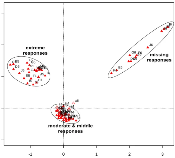
relevance of CA and MCA. Figure 1 shows the MCA of the Spanish data for the questions in

Table 1. Three clusters of response categories are evident: all the missing categories at upper

right, all the moderate responses (“agree” and “disagree”) and middle responses (“neither agree

nor disagree”) in a bunch near the origin (these are the most frequent responses), and all extreme

responses (“strongly agree” and “strongly disagree”) at upper right. A demographic variable,

age group, with six categories from young to old, a1 (16-25 years) to a6 (more than 65 years), is

MCA of questionnaire data such as these: the missing responses dominate as well as response

styles (moderate versus extreme, independent of the fact that several questions have reverse

wording) and a supplementary variable has categories only slightly separated spatially.

Figure 1: MCA of 11 questions from ISSP (1994), Spanish sample (N = 2494), with age group variable as supplementary – the supplementary age categories are all close together near the centre of the map (e.g., the labels a1, a5 and a6 are just visible, with the oldest age group a6 tending in the direction of the missing responses).

Suppose that we wanted to see the map of the response categories specifically in their relation to

the age groups. This can be achieved by constraining the solution space to be defined by the age

categories, that is performing a CCA on the indicator matrix of the 11 questions (66 dummy

variables), with the indicator matrix of the age groups (6 dummy variables) as the constraining

variables. This CCA is identical to the CA of the concatenated matrix of all cross-tabulations of

the 11 questions with the age variable, that is the matrix with 66 rows and 6 columns with the 11

-1 0 1 2 3 -1 0 1 2 3 A1 A2 A3 A4 A5 A6 B1 B2 B3 B4 B5 B6 C1 C2 C3 C4 C5 C6 D1 D2 D3 D4 D5 D6 E1 E2 E3 E4 E5 E6 F1 F2 F3F4 F5 F6 G1 G2 G3 G4 G5 G6 H1 H2 H3H4 H5 H6 I1 I2 I3 I4 I5 I6 J1 J2 J3 J4 J5 J6 K1 K2 K3 K4 K5 K6 a1 a2a3 a4a5 a6 missing responses

moderate & middle responses extreme

cross-tables stacked one on top of another. This result follows from the fact that CCA is

equivalently defined as the CA of the weighted averages of the conditioning variables for each

response category (see, for example, Greenacre, 2007: 191–192). This simplifying result

appears not be well-known: for example, Nishisato’s “forced classification” (Nishisato, 1984,

2006) is identical to the CCA described here, which in turn is identical to the CA of the stacked

tables. Figure 2 shows the CA of the stacked tables, which is more efficiently performed than

the CCA of the large indicator matrices.

Figure 2: CA of cross-tabulations of 11 questions with age groups. The standard biplot scaling is used (Greenacre, 2007: chapter 13).

In Figure 2 the domination of the response styles seen in Figure 1 has vanished and we pick up

the liberal-to-traditional scale from left to right in the response categories, with the reversely

worded questions lining up as we would expect: for example, the most spread-out question is in

-0.6 -0.4 -0.2 0.0 0.2 0.4 0.6 -0 .4 -0 .2 0 .0 0 .2 0 .4 0 .6 a1 a2 a3 a4 a5 a6 A1 A2 A3 A4 A5 A6 B1 B2 B3 B4 B5 B6 C1 C2 C3 C4 C5 C6 D1 D2 D3 D4 D5 D6 E1 E2 E3 E4 E5 E6 F1 F2 F3 F4 F5 F6 G1 G2 G3 G4 G5 G6 H1 H2 H3 H4 H5 H6 I1 I2 I3 I4 I5 I6 J1 J2 J3 J4 J5 J6 K1 K2 K3 K4 K5 K6

favour of men working and women staying at home, question I (see Table 1), from I5 on the left

to I1 on the right, while question A in favour of women working goes in the opposite direction.

Notice that all the missing value categories are on the right, in the direction of the older

respondents.

4. Constraints for dealing with missing responses

CCA can be used to focus on, or partial out, an external variable or variables. In Figure 1 we

have all the missing response categories defining a diagonal spread of points, very dominant in

the analysis because of the high association amongst missing responses on different questions.

To avoid deleting cases that have missing responses from the study, Greenacre and Pardo

(2006a, 2006b) proposed a subset version of correspondence analysis to choose subsets of

categories for visualizing – for example, this approach can be used to select all substantive

response categories and ignore the missing ones. The present approach is an alternative strategy

where we define external variables for constraining the solution. There are different ways of

doing this, and we show just one of the alternatives where the constraining variable is defined as

the count of missing responses for each respondent. For example, a respondent with no missing

respondents gets value 0, with one missing response 1, and so on, with respondents giving

missing responses to all 11 questions getting a value 11. If we constrain the MCA solution to be

linearly related to this single variable we obtain a one-dimensional CCA solution*.

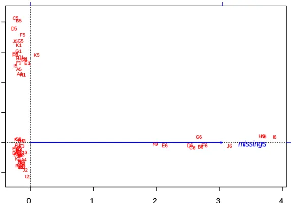
Figure 3 shows this solution as the horizontal axis (labeled ‘CCA1’), and the second axis is the

optimal first axis of the unconstrained solution (labeled ‘CA1’). Comparing this map to Figure

1 we see that the constraint has forced the missing categories to coincide with the first axis. The

*

Matschinger and Angermeyer (2006) also use the missing value counts in order to take care of missing responses – the count variable is added as a categorical variable (i.e., with as many categories as levels of counts) to each of the questions of the questionnaire and then generalized canonical analysis is used with a restriction to concentrate the missing count categories onto a single dimension. The approach is different but the idea is the same: to partial out the missing responses to avoid having to delete cases with missing data.

variable “missings” that we created, is the sum of the 11 columns of the indicator matrix

corresponding to the missing categories, hence its position in space is the average of these

categories, as shown by the vector in Figure 3 corresponding to the constraining variable.

Figure 3: CCA of 11 questions constrained by number of missings, which is a point vector lying at the average of the 11 dummy variables for the missing categories. This vector is constrained to be the first axis in the CCA.

In this sense CCA is acting like a target rotation of the MCA solution and concentrates the high

association of the missing responses on a single dimension. The remaining unconstrained

dimensions are orthogonal to this dimension and so the missing response effect has been

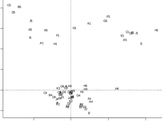
partialled out. Figure 4 shows axes 2 and 3, the first two unconstrained axes of the CCA – the

first unconstrained axis has been maintained vertical as in Figure 3, so that Figure 4 is a rotation

of the solution in Figure 3 around the vertical axis, bringing into view the next dimension

(labeled ‘CA2’) on the horizontal axis. The vertical separation is the more important one,

separating out the response styles, but now we manage to recover the liberal-traditional

0 1 2 3 4 -0 .5 0 .0 0 .5 1 .0 1 .5 2 .0 CCA1 C A 1 A1 A2 A3 A4 A5 A6 B1 B2 B3 B4 B5 B6 C1 C2 C3 C4 C5 C6 D1 D2 D3 D4 D5 D6 E1 E2 E3 E4 E5 E6 F1 F2 F3_F4 F5 F6 G1 G2 G3 G4 G5 G6 H1 H2 H3 H4 H5 H6 I1 I2 I3 I4 I5 I6 J1 J2 J3 J4 J5 J6 K1 K2 K3 K4 K5 K6 missings 0 1 2 3 4 -0 .5 0 .0 0 .5 1 .0 1 .5 2 .0 CCA1 C A 1 0 1 2 3 4 -0 .5 0 .0 0 .5 1 .0 1 .5 2 .0 CCA1 C A 1 A1 A2 A3 A4 A5 A6 B1 B2 B3 B4 B5 B6 C1 C2 C3 C4 C5 C6 D1 D2 D3 D4 D5 D6 E1 E2 E3 E4 E5 E6 F1 F2 F3_F4 F5 F6 G1 G2 G3 G4 G5 G6 H1 H2 H3 H4 H5 H6 I1 I2 I3 I4 I5 I6 J1 J2 J3 J4 J5 J6 K1 K2 K3 K4 K5 K6 missings

dispersion along the horizontal axis, for the extreme responses at the top, and for the moderate

and middle responses at the bottom.

Figure 4: CCA of 11 questions after partialling out the variable “missings” that counts the missing response categories. The missing categories (numbered ‘6’) are now all near the origin and play almost no role in the solution.

5. Discussion

In these analyses we have not reported inertias on the principal axes and their percentages. It is

known that in MCA these values are severe under-estimates of the variance accounted for, and

adjustments have been proposed by Greenacre (1988, 1995) to correct for this. For example, in

Figure 1 the inertias on the first two axes in the “classic” MCA of the indicator matrix are 0.391

and 0.384. Since the total inertia of the indicator matrix† is a fixed value of 5, the percentages of

inertia are 7.8% and 7.7%, while the adjusted values are 33.7% and 32.1% respectively. In

†

The total inertia in the MCA of an indicator matrix with Q categorical variables and a total of J categories is (J–Q)/Q, hence in this example it is (66–11)/11 = 5 (see, for example, Greenacre, 2007: chapter 18). For a definition of the adjustment, see Greenacre, 2007: chapter 19.

-1 0 1 2 -0 .5 0 .0 0 .5 1 .0 1 .5 2 .0 CA2 C A 1 A1 A2 A3 A4 A5 A6 B1 B2 B3 B4 B5 B6 C1 C2 C3 C4 C5 C6 D1 D2 D3 D4 D5 D6 E1 E2 E3 E4 E5 E6 F1 F2 F3 _F4 F5 F6 G1 G2 G3 G4 G5 G6 H1 H2 H3 H4 H5 H6 I1 I2 I3 I4 I5 I6 J1 J2 J3 J4 J5 J6 K1 K2 K3 K4 K5 K6

Figure 2, the total inertia of the CA is equal to 0.0857, which is identical to the inertia in the

constrained CCA solution of the indicator matrix, accounting for only 1.7% of the total inertia of

the indicator matrix. Similarly, in Figure 3 the constrained part of the inertia is 0.383, 7.7% of

the total inertia, while in Figure 4 the two subsequent unconstrained axes have values 0.387 and

0.305, with percentages 7.7% and 6.1% respectively. All these percentages are low owing to the

inflated value of the total inertia of the indicator matrix, but how to adjust in these alternative

situations is not immediately clear and is an open problem. Adjustment may be possible if

canonical MCA could be phrased in terms of the Burt matrix, similar to the way the adjustment

is made for ordinary MCA, where total inertia is taken to be the average of the Burt matrix’s

off-diagonal cross-tabulations.

We have shown how CCA can be used to incorporate external information into MCA results or

to treat specific response categories in survey data by imposing linear constraints on the solution

space. The map can be concentrated on the display on these variables or categories, or their

effects can be partialled out. We are also using this approach fruitfully to study the “middle”

response categories (Greenacre and Pardo, 2008) and their relationship to demographic

variables, as well as to partial out acquiescence effects which are rife in questionnaire data.

Computing note

The ca and vegan packages in R (R development core team, 2008) were used to perform the

analyses and maps in this article – for ca see Nenadić and Greenacre (2007), and for vegan, a

References

Greenacre, M. (1988). Correspondence analysis of multivariate categorical data by weighted

least squares, Biometrika, 75, 457–467.

Greenacre, M. (1995). Multivariate generalisations of correspondence analysis. In Cuadras,

C.M. and Rao, C.R. (eds), Multivariate Analysis: Future Directions 2. North Holland,

Amsterdam, pp. 327–340.

Greenacre, M. (2006). From simple to multiple correspondence analysis. In Greenacre, M. &

Blasius, J. (eds), Multiple Correspondence Analysis and Related Methods. Chapman &

Hall/CRC Press, London, pp. 41–76.

Greenacre, M. (2007). Correspondence Analysis in Practice. Second Edition. London: Chapman

& Hall / CRC Press. Published in Spanish translation as La Práctica del Análisis de

Correspondencias, Fundación BBVA, Madrid, 2008.

Greenacre, M. and Pardo, R. (2006a). Subset correspondence analysis: visualization of selected

response categories in a questionnaire survey, Sociological Methods and Research,35, 193–

218.

Greenacre, M. and Pardo, R. (2006b). Multiple correspondence analysis of subsets of response

categories. In Greenacre, M. & Blasius, J. (eds), Multiple Correspondence Analysis and

Related Methods. Chapman & Hall/CRC Press, London, pp. 197–217.

Greenacre, M. and Pardo, R. (2008). Positioning the “middle” categories in survey research: a

multidimensional approach. Keynote address at the joint conference of the European

Methodology Association and the Society for Multivariate Analysis in the Behavioural

ISSP (1994), Family and Changing Gender Roles II. International Social Survey Programme.

URL http://www.issp.org

Matschinger, H. and Angermeyer, M.C. (2006). The evaluation of “don’t know” responses by

generalized canonical analysis. In Greenacre, M. & Blasius, J. (eds), Multiple

Correspondence Analysis and Related Methods. Chapman & Hall/CRC Press, London, pp.

283–298.

Nenadić, O. and Greenacre, M. J. (2007). Correspondence analysis in R, with two- and

three-dimensional graphics: The ca package. Journal of Statistical Software, 20 (1).

URL http://www.jstatsoft.org/v20/i03/

Nishisato, S. (1984). Forced classification: a simple application of a quantification technique.

Psychometrika, 49, 25–36.

Nishisato, S. (2006). Multivariate Nonlinear Descriptive Analysis. London: Chapman &

Hall/CRC Press, London.

Oksanen J., Kindt R., Legendre P. & O'Hara R.B. (2006). vegan: Community Ecology Package

version 1.8-3. URL http://cran.r-project.org/

R Development Core Team (2008). R: A Language and Environment for Statistical Computing.

R Foundation for Statistical Computing, Vienna, Austria.

URL http://www.R-project.org

Ter Braak, C.J.F. (1986). Canonical correspondence analysis: a new eigenvector technique for