Testing for PPP: Should We Use Panel Methods?

(1)

Testing for PPP:

Should We Use Panel Methods?

¤

Anindya Banerjee

y

_{Massimiliano Marcellino}

z

_{Chiara Osbat}

x

Abstract

A common …nding in the empirical literature on the validity of purchasing power parity (PPP) is that it holds when tested for in panel data, but not in univariate (i.e. country speci…c) analysis. The usual explanation for this mis-match is that panel tests for unit roots and cointegration are more powerful than their univariate counterparts. In this paper we suggest an alternative ex-planation for the mismatch. More generally, we warn against the use of panel methods for testing for unit roots in macroeconomic time series. Existing panel methods assume that cross-unit cointegrating or long-run relationships, that tie the units of the panel together, are not present. However, using empirical examples on PPP for a panel of OECD countries, we show that this assumption is very likely to be violated. Simulations of the properties of panel unit root tests in the presence of long-run cross-unit relationships are then presented to demonstrate the serious cost of assuming away such relationships. The empirical size of the tests is substantially higher than the nominal level, so that the null hypothesis of a unit root is rejected very often, even if correct.

J.E.L. Classi…cation: C23, C33, F31

Keywords: PPP, unit root, panel, cointegration, cross-unit dependence

¤_{We wish to thank Ronnie MacDonald for helpful comments. The …nancial support of the} European University Institute in funding this research is also gratefully acknowledged.

y_{Corresponding author. Department of Economics, European University Institute, 50016} San Domenico di Fiesole. Phone: +39-055-4685-356. Fax: +39-055-4685-202. E-mail: [email protected]

z_{Istituto di Economia Politica and IGIER, Universita’ Bocconi, Via Salasco 3, 20136 Milano} x_{Department of Economics, European University Institute, 50016 San Domenico di Fiesole.}

(2)

1 Introduction

The last few years have seen a veritable explosion of papers on testing for purchasing power parity (PPP) using panels of macroeconomic data. A selection would include

inter alia Mark (1995), Frankel and Rose (1995), Jorion and Sweeney (1996), Oh (1996), Rogo¤ (1996), O’Connell (1998), Papell (1997), and more recently Bayoumi and MacDonald (1999), Pedroni (1999a) and the papers by Papell and co-authors given below.

The real dollar (or Deutsche mark) exchange rate for countryiis constructed as:

qit =eit+p¤t¡pit;

where qit is the logarithm of the real exchange rate, p¤t is the logarithm of the US

(or German) CPI andpt is the logarithm of the CPI for countryi. The strong form

of the test for PPP consists of testing the null of a unit root in theqit series, either

individually (i.e. country by country) or using panel methods, discussed brie‡y in the next section.

More generally, a weak form of the hypothesis may be tested by constructing the series eqit, where

e

qit =eit+®p¤t ¡¯pit:

An acceptance of a unit root in the seriesqeit is taken to be a rejection of the weak

form of the PPP hypothesis. The® and¯ can be either taken to be knowna priori or derived from single-equation- or system-cointegration methods, since all three component series ofq_eit are assumed to be I(1). The test of the weak form in panels

may thus be seen to be tests for cointegration in panel data.

Among the large number of papers available in the literature, special attention should be drawn to the work of Papell and his co-authors who have investigated and drawn attention to a large number of issues that are relevant to a proper consider-ation of the evidence derived from panel tests.

The starting-o¤ point for the use of panel unit root and panel cointegration tests is the presumption that univariate (i.e country-speci…c) tests have low power. Within this framework, Papell (2000) for example has noted that the use of panel tests does not always rescue the various forms of the PPP hypothesis. In particular, Papell and Theodoridis (2000) …nd that the choice of the numeraire currency is important in determining rejections or acceptance of a unit root in the real exchange rate series. Using a recursive estimation exercise, they show that the choice of the Deutsche mark as the numeraire currency leads to rejections of the unit root hypothesis for

(3)

sample sizes of steadily increasing lengths (with a …xed starting point) much more strongly than when the dollar is taken to be the numeraire.

Papell (2000) argues in favour of the use of methods analogous to those em-ployed by Perron (1989) in his much-cited paper that introduced the possibility of deterministic breaks in tests for unit roots. Papell showed that by modelling the appreciation and then depreciation of the dollar in the 1980’s as shifts in the deter-ministic components of the series, stronger rejections of the unit root hypothesis in real exchange rate series are obtained. While the experience with such models in a purely time-series context does not make this a particularly surprising …nding, it nevertheless alerts us to some of the subtleties that need to be tackled in determining whether or not weak- or strong-form PPP holds in the data.

The origin of our research in this paper is the evidence presented in Banerjee, Marcellino, and Osbat (2000) (BMO). There we investigated the properties of tests of cointegration in panels of data, particularly those proposed by Groen and Kleiber-gen (1999) and Larsson and LyhaKleiber-gen (1999), and showed that not taking account of the cointegrating relationships across the units of the panel would lead to serious di¢culties in inference about cointegration within the units of a panel. These tests are extensions to panels of the Johansen approach to estimating cointegrating rank among time series, and the main restriction imposed is that there are no cointe-grating relationships among the variables across the units (typically countries) of the panel. We showed that when this restriction is valid, the tests have the correct size and high power to detect cointegration. If the restriction is invalid however, the tests for cointegration tend to be grossly over-sized especially as T increases, so that the null of no cointegration is rejected too often in relation to the nominal con…dence level (or size) of the test.1

In the context of the equations above, the panel approach (both to testing for unit roots and cointegration) as currently advocated, rules out the existence, for example, of cointegrating relationships between eit and ejt or pit and pjt, for all

i 6= j. In this paper we demonstrate the consequences of the violation of this

assumption by looking at the properties of the panel unit root tests commonly used to test for stationarity of the real exchange rate. We show that over-sizing is a major problem also here. While the analysis in BMO is therefore more directly relevant for the consideration of the weak form of PPP, our main aim here is to explore further the arguments within the context of the strong form of the PPP hypothesis:

1_{This over-sizing property of panel unit root tests has also been discussed by Engel (2000)}

and O’Connell (1998) in slightly di¤erent contexts. Engel’s paper does not deal with panels while O’Connell shows the e¤ect ofshort-run linkages among the units (for example through the non-zero covariances of the errors across the units) on unit root tests.

(4)

In the next section, we provide a brief overview of three of the most commonly used tests for unit roots in panels. These are the Levin and Lin (1992) and Levin and Lin (1993) (LL), Im, Pesaran, and Shin (1997) (IPS) and Maddala and Wu (1999 Special Issue) (MW) tests. More comprehensive summaries are providedinter alia

by Baltagi and Kao (2000) and Banerjee (1999), and readers not interested in tech-nical details may skip this section. Section 3 provides a set of motivating empirical examples demonstrating that while unit-by-unit ADF tests typically tend to accept the null of a unit root for the real exchange rate, panel unit root tests often reject this null. Such rejections must however be treated with a great deal of caution since there is strong evidence, detailed here, of cross-unit or cross-country cointegrating relationships. Therefore, in the light of our discussion above, these rejections instead of being attributed to the higher power of panel unit root tests may be attributed simply to the over-sizing that is present when cointegrating relationships link the units of the panel together. This claim is demonstrated in more detail in section 4 with a set of Monte Carlo experiments that analyze the size and power properties of the LL, IPS and MW tests in a series of cases. The cases studied include notably the presence or absence of cross-unit cointegration and the presence or absence of weak exogeneity of some of the variables. Section 5 o¤ers conclusions and closing remarks.

2 Testing for Unit Roots in Dynamic Panels

2.1 Levin and Lin (1992, 1993)

The model adopted by Levin and Lin allows for …xed e¤ects and unit-speci…c time trends in addition to common time e¤ects (which may in practice be concentrated out of the equation) and is given by

¢yit=®i+±it+µt+½iyit¡1+³it; i= 1;2; :N; t= 1;2; :::; T: (1)

The null hypothesis of interest is H0: ½i = 0 for all i against the alternative HA:

½i =½ <0 for alli.

Levin and Lin (1992) derive the asymptotic distributions of the panel estimator of ½ under di¤erent assumptions on the existence of …xed e¤ects or heterogeneous time trends. For example, if³it »IID(0; ¾2)for …xedi;the errors are also assumed

to be independent across the units of the sample, ®i = ±i = 0 for all i and there

(5)

squares (OLS) pooled panel estimator and associatedt-statistic are given by

TpNb½ =) N(0;2); T; N ! 1 (2) t½=0 =) N(0;1):

Note that, compared to unit-by-unit Dickey-Fuller tests, the LL statistics have (a) a faster rate of convergence to their asymptotic distributions and (b) the limiting distributions are normal.

In a slightly more general model, where®i 6= 0; ±i = 0 in (1),

TpN_b½+ 3pN =) N(0;10:2);pN=T !0; T; N ! 1 (3)

p

1:25t½=0+

p

1:875N =₎ N(0;1);pN=T _!0; T; N _{! 1}:

The null hypothesis for this second model is given by H0 : ½ = 0; ®i = 0 for all i

against the alternativeHA :½ <0; ®i unrestricted.

As a further generalisation, let us now consider the second of the two models dis-cussed above with the error process following a stationary invertible ARMA process for each unit but still being distributed independently across units. Thus,

³it =

1

X

j=0

µij³it¡j +"it; t= 1;2; :::T: (4)

A multi-step procedure is prescribed by Levin and Lin (1993) for this case. The starting point is the application of augmented Dickey-Fuller (ADF) test to each individual series. Thus, the regression

¢yit =®i+½iyit¡1+

pi

X

j=1

µij¢yit¡j +"it; i= 1;2; :N; t= 1;2; :::T (5)

is estimated (for each i) by regressing …rst ¢yit and then yit¡1 on the remaining regressors in the ADF regression above, providing the residuals_beit andVbit¡1 respec-tively. Then the regression of_beit onVbit¡1

b

eit =½iVbit¡1+"it (6)

is estimated to derive_b½_i from the i-th cross-section. The following expressions are next required:

(6)

b ¾2_e_i = (T _¡pi¡1)¡1 T X t=pi+2 (_beit¡b½iVbit¡1)2 (7) e eit = beit=b¾ei e Vit¡1 = Vbit¡1=b¾ei b ¾2_y_i = (T ¡1)¡1 T X t=2 ¢y_it2 + 2 K X L=1 w_KL Ã (T ¡1)¡1 T X t=L+2 ¢yit¢yit¡L) !2 b SNT = N¡1 N X i=1 (_b¾yi=b¾ei);

whereK is the lag truncation parameter and w_KL = (L=(K+ 1)).

The …nal step is to estimate the panel regression (making use of alli andt)

e

eit=½Veit¡1+"eit (8)

and compute thet-statistic

t½=0 = b ½ RSE(_b½); (9) where RSE(_b½) = _b¾" " _N X i=1 T X t=pi+2 e V_it2_¡₁ #¡1=2 (10) b ¾2_" = (NTe)¡1 N X i=1 T X t=pi+2 (_eeit¡b½Veit¡1)2 p = N¡1 N X i=1 pi; Te= (T ¡p¡1):

The Levin and Lin statistic is an adjusted version of the t-statistic above and is given by

t¤½=

t½=0¡NTeSbNT¾b"¡2RSE(b½)e¹Te

¾_T_e ; (11)

where ¹eTe and , ¾Te are mean and standard deviation adjustment terms which are

computed by Monte Carlo simulation and tabulated in their paper for three separate speci…cations of the deterministic terms above.

The main result of the Levin and Lin analysis is that under the null hypothesis that ½= 0, the panel test statistic t¤½ has the property that

(7)

provided the ADF lag order pmax increases at some rate Tp where 0 < p · 1=4 and the lag truncation parameter K increases at rate Tq _where ₀ _{< q <} ₁_{. Under}

the alternative hypothesis,t¤½ diverges to negative in…nity at rate

p

NT, a property that can thereby be exploited to construct a consistent one-tailed test of the null hypothesis against the alternative.

2.2 Im, Pesaran and Shin (1997)

Im, Pesaran, and Shin (1997) extend the Levin and Lin framework to allow for heterogeneity in the value of½_i under the alternative hypothesis. Let

¢yit =®i+½iyit¡1+³it; i= 1;2; :::; N;t = 1;2; :T; (13)

where the errors³_it are serially autocorrelated with di¤erent serial correlation (and variance) properties across the units. The null and alternative hypotheses are given byH0 :½i = 0 for all i; against the alternativeHA :½i <0; i = 1;2; :::; N1; ½i = 0;

i=N1+ 1; N1+ 2; :::N:

Following the critique of Pesaran and Smith (1995) on pooled panel estimators, such as those used by Levin and Lin (1992) and Levin and Lin (1993), Im, Pesaran, and Shin (1997) propose a group-mean Lagrange multiplier (LM) statistic. The ADF regressions ¢yit =®i+½iyit¡1+ pi X j=1 µij¢yit¡j +"it; t = 1;2; :::T (14)

are estimated for eachiand the LM-statistic for testing½i = 0is computed. De…ning

LMN;T =N¡1 N

X

i=1

LMiT(pi;µi); (15)

whereµi = (µ11; µ12; :::µ1pi)0 andLMiT(pi;µi)is the individualLM-statistic for

test-ing½_i = 0, the standardized LM-bar statistic is given by

ªLM = p NnLMN;T ¡ N¡1PN_i₌₁E[LMiT(pi;0j½i = 0] o q N¡1PN i=1V ar[LMiT(pi;0j½i = 0] : (16)

The values of E[LMiT(pi;0j½i = 0] andV ar[LMiT(pi;0j½i = 0] are obtainable by

stochastic simulation and are tabulated in their paper using 50,000 replications for di¤erent values ofT andpi’s.

Im, Pesaran, and Shin (1997) show that under H0: ½i = 0for alli,

(8)

asT; N ¡! 1andN=T ¡!k where k is a …nite positive constant. For the test to be consistent under the alternative, it is also required that lim N¡!1(Ni=N) =¸1;

0 < ¸1 · 1. Under this further assumption, ªLM diverges to positive in…nity at

rate TpN under the alternative.

Im, Pesaran, and Shin (1997) also propose the use of a group-meant-bar statistic given by ªt= p NntN;T ¡ N¡1PNi=1E[tiT(pi;0j½i = 0] o q N¡1PN i=1V ar[tiT(pi;0j½i = 0] (18) where, tN;T =N¡1 N X i=1 tiT(pi;µi) (19)

andtiT(pi;µi)is the individualt-statistic for testing½i = 0for alli: E[tiT(pi;0j½i = 0]

andV ar[tiT(pi;0j½i = 0]are tabulated in the paper. The convergence result stated

for ªLM holds for ªt also, and consistency is guaranteed under the controlled rate

of divergence ofN andT to in…nity.

In a Monte Carlo study, Im, Pesaran, and Shin (1997) demonstrate better …nite sample performances of the ªLM andªt tests in relation to the Levin and Lin test

given by t¤_½. We undertake a comparison of these tests in section 4 below for our various cases of interest. In the comparison we also include the Maddala and Wu test, which is described next.

2.3 Maddala and Wu (1999)

Maddala and Wu, relying on Fisher (1932), suggest combining the p-values of a test-statistic for a unit root in each cross-sectional unit. The Fisher test is an exact and non-parametric test, and may be computed for any arbitrary choice of a test for the unit root in a cross-sectional unit. The statistic is given by

M W :¡2

N

X

i=1

ln(¼i);

and is distributed as a chi-squared variable with 2N degrees of freedom under the assumption of cross-sectional independence. ¼i is the p-value of the test statistic in

unit i, the p-value of the ADF test statistic in the cases that we consider.

The obvious simplicity of this test and its robustness to the choice of lag length and sample size make its use attractive. However, our experience with the MW test is somewhat less encouraging, as reported below.

(9)

3 Testing for PPP

In this section we evaluate empirically whether the strong version of the purchasing power parity (PPP) holds, namely, whether the real exchange rate (rer) is stationary. This question has attracted considerable interest, as mentioned in the Introduction. Following Pedroni (1999b) and Mark (1995), we use quarterly data on nominal exchange rates andcpi, for the period 1973:1-1997:4, for 19 OECD countries.

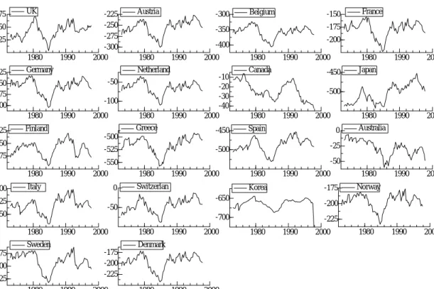
The rers when US is used as the numeraire country are graphed in Figure 1. Note that the nominal exchange rates are expressed as US$ per national currency, so that a decline in the rer corresponds to a depreciation of the national currency. It is di¢cult to determine from the graphs whether therers are stationary or not, but it is evident that most rers tend to move together, in particular for the countries currently in the European Monetary Union. This suggests that if the rers are integrated, they are also cointegrated across countries.

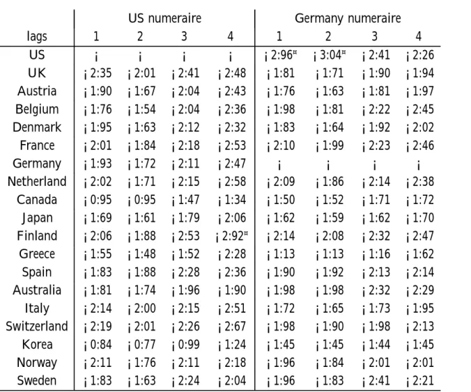
The augmented Dickey-Fuller (ADF) test accepts the null hypothesis of a unit root in therer for each country and any choice of lag length, see Table 1.

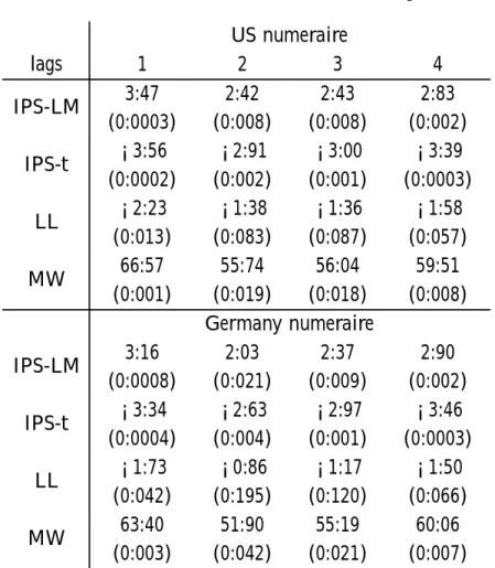
The results of the panel unit root tests are reported in Table 2. Both versions of the IPS tests and the MW statistic reject the presence of a unit root at the 5% signi…cance level, while the LL test in general accepts. Overall, on the basis of the panel tests we would conclude that PPP holds. Yet, before drawing such a conclusion, we should check that the countries under analysis are not linked by cointegrating relationships, an important hypothesis underlying all panel unit root tests (for the tests to have correct size).

As mentioned earlier, it may be seen from Figure 1 that there appear to be substantial comovements of the rers across countries. To evaluate more formally whether therers are cointegrated, we calculate the Johansen trace test for the rers of all pairs of countries, using in each case a VAR(4) with an unrestricted constant to model the variables (the outcome is not sensitive to the choice of the lag length). The results are reported in Table 3. In many cases the null hypothesis of no bivariate cointegration is rejected at the 10% and also at the 5% signi…cance level. Given that this test can be also expected to be biased toward acceptance of the null hypothesis in small samples, even more cross-country cointegration can be presumed to exist.2 Another interesting tool to analyze jointly the properties of large systems of possibly non-stationary variables was developed by Gonzalo and Granger (1995). It allows the determination of the total number of nonstationary trends driving all the variables under analysis. To implement this procedure, …rst we extract the

2_{If the}_{rers were stationary, the hypothesis of cointegrating rank equal to one versus rank equal}

(10)

common trend from each of 7 bivariate systems that are cointegrated according to Table 3 (UK-Austria, Belgium-Netherlands, France-Germany, Japan-Australia, Finland-Norway, Spain-Italy, Greece-Switzerland). Then, we extract the trends from a 4-variable system for Denmark, Canada, Korea and Sweden. The rers for these countries turn out not to be cointegrated, hence we have 4 additional stochastic trends. Finally, we test for cointegration among the 11 trends (7 obtained in the …rst step plus the 4 trends obtained in the second step) using the Johansen trace statistic in a VAR(3). The hypothesis of cointegrating rank equal to 5 is accepted at the 10% level, while that of rank equal to 4 is accepted at the 5% level. Hence, on the basis of the Gonzalo and Granger (1995) procedure, only 6 or 7 stochastic trends drive the joint evolution of the 18rers. As a consequence, there exist 12 or 11 cointegrating relationships among the rers.

Both the bivariate cointegration analysis and the Gonzalo and Granger procedure indicate the presence of many cointegrating relationships across the countries, so that a basic assumption underlying the panel unit root tests is violated. The simulations in the next section show that in this case the panel tests can be substantially biased. The actual size is much larger than the nominal level, i.e. the null hypothesis of a unit root is rejected too often, and this can help to explain the con‡icting outcomes of the univariate and panel unit root tests. From the results of the simulation experiments in Tables 10 and 13 for T = 100, whose parameters are very close to

those of our empirical analysis, it may be seen that LL is the least distorted panel test. Indeed this is the test which accepts the null hypothesis of a unit root at the 5% level for our empirical example, in agreement with the unit by unit ADF tests, and provides evidence against the validity of the strong version of PPP.3

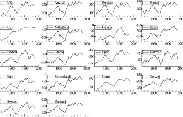
According to Papell and Theodoridis (2000), the choice of thenumeraire country can a¤ect the procedures to evaluate the presence of PPP in the long run. Hence, we repeat our analysis using Germany as the numeraire. The resulting rers are graphed in …gure 2. Though there are some changes with respect to the graphs in Figure 1, the overall pattern is quite similar.

The ADF test still accepts the null hypothesis of a unit root in therer for each country, see Table 1. The IPS and the MW panel tests reject this hypothesis, while the LL statistic accepts it, see Table 2. As for the case with US as thenumeraire, both the graphs in …gure 2 and the formal bivariate cointegration analysis indicate the presence of several cross-country cointegrating relationships among the rers,

3_{Alternative explanations for the failure of Levin and Lin tests to reject the null hypothesis of a}

unit root have been proposed by Papell (2000), as discussed in the introduction to this paper. In some sense these arguments must be weighed o¤ against those proposed here since these provide grounds for over-rejection of the null.

(11)

see Table 4, even though the pattern of bivariate cointegration is di¤erent when Germany is thenumeraire. The presence of cross-country cointegrating relationships among the rers is also con…rmed by the Gonzalo and Granger method. Applying the step-wise procedure we described before, it turns out that in this case only 3 or 4 stochastic trends drive the evolution of the 18 rers.4 _{Hence, the panel tests can} be even more biased towards over-rejection in this case.

In summary, the unit by unit ADF tests favor the hypothesis of a unit root in the real exchange rates, while the IPS and MW panel unit root tests reject this hypoth-esis. This mismatch can be due to a bias in the panel tests, that reject too often the presence of a unit root when there are cross-unit cointegrating relationships. The panel LL test appears to be more robust in this case, and indeed it accepts the presence of a unit root, in agreement with the ADF tests. These …ndings are robust to the choice of the numeraire country, which instead in‡uences the number and composition of the cross-country cointegrating relationships.

4 Simulation results for panel unit root tests

In this section we describe the Monte Carlo design, and then evaluate the per-formance of the panel unit root tests, with and without cross-unit cointegrating relationships. This provides evidence on the reliability of the panel methods when applied to test for PPP and, more generally, to evaluate the stationarity of macroe-conomic time series for several countries.

4.1 The Monte Carlo Design

Let us consider the variables yit, xit, where i = 1; :::N indexes the units and t =

1; :::; T is the temporal index. We group the y and x variables for each unit into theN £1 vectors Yt = (y1t; :::; yNt)0 and Xt = (x1t; :::; xNt)0. Then we consider the

following Error Correction Model (ECM) as the data generating process (DGP):

Ã ¢Yt ¢Xt ! =®¯0 Ã Yt¡1 Xt¡1 ! +"t; (20)

4_{We consider in the …rst step 7 bivariate VARs(4), for the pairs US-UK, Austria-Switzerland,}

France-Spain, Australia-Japan, Finland-Norway, Netherland-Sweden, and Greece-Denmark. Then we analyze a 4-variable VAR(4) for Belgium, Canada, Italy and Korea, but no cointegrating rela-tionships are found. Finally, we run a VAR(3) for the 7 stochastic trends we obtain in the …rst step, plus the 4 trends from the second step. The cointegrating rank is 7 or 8 when using 5% or 10% critical values, so that 4 or 3 stochastic trends drive the 18 rers.

(12)

where"t isi:i:d: N(0;§), with § = 0 B B B B @ ¾1 0 ¢ ¢ ¢ 0 0 ¾2 :::: 0 ... ... ... 0 0 _{¢ ¢ ¢} ¾2N 1 C C C C A;

and¾j is extracted from a uniform distribution on[0:5;1:5], for j = 1; :::;2N.

We also consideredDGPs with lagged di¤erences as regressors and serially cor-related errors. There were no qualitative di¤erences in the results, and hence we focus on the speci…cation in (20). The di¤erent experiments for size and power, with or without cross unit cointegration, are obtained by imposing proper restrictions on the® and¯ matrices, as detailed below. In all cases the results are based on 5000 replications, and are reported for di¤erent values of N (5, 10, 25, 50, 100) and of T (25, 50, 100), to mimic situations often encountered in empirical applications.

4.2 No cross-unit cointegration

The …rst case we consider is testing for unit roots when there are no cross-unit coin-tegrating relationships,i.e., we are in a situation where the assumptions underlying panel tests hold. We are interested in evaluating the small sample size and power of the tests, to have a benchmark for the other cases.

For the size experiments we set ® = 0 in the DGP, so that Xt and Yt are

independent random walks. For the power experiments we use ®= 0 @ NI£N N£IN 0 N£N N£0N 1 A; ¯0 = 0 @ N¡£IN N£0N c I N£N N£0N 1 A;

wherec= 0:9 orc= 0:8. Hence,Xt is an N variate random walk, whileYt is made

up ofN stationary AR(1) processes, with roots equal to c. The estimated model for each unit is

¢yit=°0yit¡1+°1¢yit¡1+°2¢yit¡2+eit: (21)

This choice re‡ects the fact that when the lag length is underspeci…ed relative to the DGP the tests become very undersized, while overspeci…cation improves the size, even though the power can deteriorate slightly. The choice of the lag truncation in computing b¾2_y_i in (7) is also important in determining size, and we follow Levin and Lin’s recommendations for comparability with existing results in the literature.

(13)

The empirical sizes of the unit root tests are reported in Table 5. We can read this table along three directions: for varyingN, for varyingT, and for bothN andT varying. For …xedT, in general the performance of the IPS-LM test improves when N increases, while it deteriorates for the IPS-t and, in particular, for the MW tests; the size is always decreasing for LL. WhenN is …xed, in general the size distortions of all tests decrease with T, and this is particularly evident for MW. When both N and T vary, we consider the cases where N=T is about 0.25 ((N = 5; T = 20), (N = 10; T = 50), (N = 25; T = 100)) or 0.5 ((N = 10; T = 20), (N = 25; T = 50), (N = 50; T = 100)). The size improvements for larger dimensions are clear, in

particular whenN=T = 0:5. Overall, the IPS-LM has very low size distortions when

N > 25 and T > 50, while the other three tests experience deviations from the

nominal level also for these rather large values of units and temporal observations. It is worth noting that the LL test performs better when N is small, less than 25.

The power results are reported in Tables 6 and 7 for, respectively, c = 0:8 and

c = 0:9. For T = 20 and N increasing, the IPS-t and the MW have the highest power, which is not surprising because of their large size distortions. The IPS-LM and the LL tests, with better size properties, have good power for N large when c= 0:8, but not for c = 0:9 (the power is less than 40% also for N = 100). When

T = 50, the situation improves substantially, in particular for the IPS-LM and

already for N = 25, also with c = 0:9. When T = 100 the power is close or equal

to one for all tests, with the exception of LL whenN = 5;10 andc= 0:9. For …xed

N, the power increases substantially with T already for N = 5, and a similar result

holds whenN and T vary jointly.

Overall, these …gures indicate that the temporal dimension is quite important for high power also in a panel context, and that the IPS-LM test has not only good empirical size but also rather high power, particularly whenN >25andT >50.5

4.3 Cross-unit cointegration, weak exogeneity

We now consider the following speci…cation of the DGP, to allow for cross-unit cointegrating relationships to be present:

®= 0:1 0 @ N¡£IN N0£N 0 N£N N¡£IN 1 A; ¯0 = 0 @ N¡£IN N£IN 0 N£N NB£N 1 A;

5_{We also considered di¤erent values for}_c_{across the units. This violates the condition of the LL}

test on the alternative hypothesis, and the LL test turns out to have systematically lower power than the IPS tests and MW in this case.

(14)

B = 0 B B B B B B B B B B B @ 1 _¡1 0 0 0 0 ::: 0 0 1 _¡1 0 0 0 ::: 0 0 0 1 _¡1 0 0 ::: 0 0 0 0 0 0 0 ::: 0 0 0 0 0 0 0 ::: 0 ::: 0 0 0 0 0 0 ::: 0 1 C C C C C C C C C C C A : (22)

Hence, all the variables areI(1), but the system is driven by a number of independent random walks equal to the number of zero rows of B, say b. For example, in the formulation in (22),b=N_¡3. The remaining2N_¡b stationary roots of the system are equal to0:9. There exist N within unit cointegrating relationships, (yit¡xit),

i= 1; :::; N, plusN¡bcross-unit cointegrating relationships of the type(xit¡xi+1t),

i = 1; :::N _¡b. Moreover, the xi variables are weakly exogenous in the subsystem

for theyi variables.6 In BMO, weak exogeneity was an important factor in reducing

the size distortions, which is our reason for considering it here. The next subsection deals with the case of cross unit-relationships but without weak exogoneity.

The estimated model for each unit remains

¢yit =°0yit¡1+°1¢yit¡1+°2¢yit¡2+eit; (23)

and we are interested in evaluating if and how the presence of cross-unit cointegration a¤ects the performance of the panel unit root tests. Note that each yi is I(1), so

that the empirical rejection frequencies of the tests should be around5%.

The results are reported in Tables 8 to 12, for di¤erent values of N and vary-ing percentages of cross-unit cointegration, q, where q = ((N _¡b)=N)_¤100. The parameter q typically ranges from 20% to 80%, i.e., from 20% to 80% of the units are related by bivariate cointegrating relationships. Five points are worth making. First, the distortions for IPS-t and MW are substantial in all cases, with values often in the range20%_¡50% when N > 25 and T = 20. Second, the IPS-LM performs reasonably well for T = 20, while the LL test appears to be quite robust to the presence of cross-unit cointegration, with only minor distortions. Third, focusing on IPS-LM and LL, when T increases the distortions increase. Fourth, the distortions decrease for larger N in the case of LL, and do not increase with N for IPS-LM. Fifth, forN >25the distortions increase with q, while for fewer units the outcome is less clear cut.

6_{Essentially this requires that the cointegrating relationships between}_y

iandxido not a¤ect the

xi variables. See Johansen (1995) for a more precise de…nition of weak exogeneity in cointegrated

(15)

4.4 Cross-unit cointegration, no weak exogeneity

We still want all the variables to beI(1), with the system driven by fewer than 2N stochastic trends and thexi variables no longer weakly exogenous in the subsystem

for the yi variables. Hence, we consider the following speci…cation of the DGP:

®= 0:1 0 @ N¡£IN N0£N A N£N N¡£IN 1 A; ¯0 = 0 @ N¡£IN N£IN B N£N N£0N 1 A; A= 0 B B B B B B B B B B B @ 1 0 0 0 0 0 ::: 0 0 1 0 0 0 0 ::: 0 0 0 1 0 0 0 ::: 0 0 0 0 0 0 0 ::: 0 0 0 0 0 0 0 ::: 0 ::: 0 0 0 0 0 0 ::: 0 1 C C C C C C C C C C C A ; B = 0 B B B B B B B B B B B @ 1 _¡1 0 0 0 0 ::: 0 0 1 _¡1 0 0 0 ::: 0 0 0 1 _¡1 0 0 ::: 0 0 0 0 0 0 0 ::: 0 0 0 0 0 0 0 ::: 0 ::: 0 0 0 0 0 0 ::: 0 1 C C C C C C C C C C C A : (24) There are 2N _¡b stationary roots equal to 0:9, where we recall that b is the number of zero rows of B (i.e., the system is driven by b stochastic trends). The stationary roots are associated withN within unit cointegrating relationships,(yit¡

xit), i= 1; :::; N, plus N¡b cross-unit cointegrating relationships of the type (yit¡

yi+1t),i= 1; :::N¡b. The cointegrating relationship betweenyi andyi+1 a¤ects xi,

which is therefore not weakly exogenous.

The estimated model for each unit remains that in equation (21).

The results are summarized in Table 13. Ranking the tests in terms of size distortions, MW is the worst, followed by IPS-t, which though performs much better than in the weakly exogenous case. IPS-LM is reasonably well behaved for T = 20

andT = 50, but still presents substantial size distortions forT = 100, that increase

with the number of units,N. The LL statistic appears again to be the most robust, with empirical size in the range 3%-8% also for T = 100 and N = 100. It may

also be noted by comparing Tables 8 to 12 with Table 13 that the lack of weak exogeneity does not pose any special problem in the context of our analysis here, while the consequences were much more serious for the results in BMO.

5 Conclusions

The empirical analysis in our paper demonstrates clearly the importance of taking proper account of the presence of cross-unit cointegrating relationships in

(16)

inter-preting the results of unit root tests in panel. These cross-unit relationships are detectable by means of bivariate or small-system cointegration analysis and by the Gonzalo and Granger (1995) procedure on the estimated common trends. Using the latter, the amount of cross-unit cointegration in the PPP panel in section 3 is found to be around 50% with US as thenumeraire and around 80% with Germany as the

numeraire country. Looking at the relevant entries of Tables 8-13, for T=100, N=25 and q=50% or 80%, the size-distortions are in the range of 0.07 to 0.32 whenxt is

weakly exogenous. When xt is not weakly exogenous, the corresponding numbers

are 0.03 and 0.24 respectively. It should also be noted that of all the tests con-sidered, the LL test appears to su¤er the least from size distortion in the presence of cross-unit cointegrating relationships, but the DGPs considered here are on the whole those most favourable to the LL testing framework because of the homogene-ity across the units of the autoregressive parameter. In some results not reported here, we also …nd that when heterogeneity is allowed for in the DGP, the power of the LL test is lower than for the other panel tests considered.

Overall, our results provide yet a further serious warning against the use of standard panel unit root tests but also a stimulus for further research. In particular, the aim should be to understand the theoretical properties of these tests under various relaxations of the underlying assumption of cross-unit long run independence and to devise procedures that are robust to such generalisations.

References

Baltagi, B., and C. Kao(2000): “Nonstationary Panels, Cointegration in Panels and Dynamic Panels: A Survey,” mimeo.

Banerjee, A.(1999): “Panel Data Unit Roots and Cointegration: An Overview,”

Oxford Bulletin of Economic and Statistics, 61, 607–630.

Banerjee, A., M. Marcellino, and C. Osbat (2000): “Some Cautions on the Use of Panel Methods for Integrated Series of Macro-Economic Data,” Discussion Paper working paper n.170, IGIER.

Bayoumi, T., and R. MacDonald (1999): “Deviations of Exchange Rates from Purchasing Power Parity: A Story Featuring Two Monetary Unions,” Discussion Paper 46, 1, IMF Sta¤ Papers.

Engel, C.(2000): “Long-Run PPP May Not Hold After All,”Journal of Interna-tional Economics, 57, 243–273.

(17)

Fisher, R. (1932): Statistical Methods for Research Workers. Oliver and Boyd, Edimburgh.

Frankel, J. A., and A. K. Rose (1995): “Empirical Research on Nominal Ex-change Rates,” in Handbook of International Economics Vol. 3, ed. by G. M. Grossman, and K. Rogo¤, pp. 1689–1729. Elsevier Science, Amsterdam.

Gonzalo, J., and C. W. J. Granger (1995): “Estimation of Common Long-Memory Components in Cointegrated Systems,” Journal of Business and Eco-nomic Statistics, 13, 27–36.

Groen, J. J., and F. R. Kleibergen (1999): “Likelihood-Based Cointegration Analysis in Panels of Vector Error Correction Models,” Discussion Paper Discus-sion Paper 55, Tinbergen Institute.

Im, K. S., M. H. Pesaran,andY. Shin(1997): “Testing for Unit Roots in Hetero-geneous Panels,” Discussion paper, Department of Applied Economics, University of Cambridge.

Johansen, S. (1995): Likelihood-Based Inference in Cointegrated Vector Autore-gressive Models. Oxford University Press, Oxford and New York.

Jorion, P., and R. Sweeney (1996): “Mean Reversion in Real Exchange Rates: Evidence and Implications for Forecasting,” Journal of International Money and Finance, August, 535–550.

Larsson, R., and J. Lyhagen (1999): “Likelihood-Based Inference in Multi-variate Panel Cointegration Models,” Discussion Paper Working Paper Series in Economics and Finance 331, Stockholm School of Economics and Finance.

Levin, A., and C. Lin (1992): “Unit Root Tests in Panel Data: Asymptotic and Finite Sample Properties,” Discussion Paper 92-93, Department of Economics, University of California at San Diego.

Levin, A.,and C. F. Lin(1993): “Unit Root Tests in Panel Data: New Results,” Discussion Paper Discussion Paper 56, University of California at San Diego.

Maddala, G., and S. Wu (1999 Special Issue): “A Comparative Study of Unit Root Tests and a New Simple Test,” Oxford Bulletin of Economic and Statistics, 61, 631–652.

Mark, N.(1995): “Exchange Rates and Fundamentals: Evidence on Long-Horizon Predictability,” American Economic Review, 85, 201–218.

(18)

O’Connell, P. G. J. (1998): “The Overvaluation of Purchasing Power Parity,”

Journal of International Economics, 44, 1–19.

Oh, K.(1996): “Purchasing Power Parity and Unit Root Tests Using Panel Data,”

Journal of International Money and Finance, 15, 405–418.

Papell, D. (1997): “Searching for Stationarity: Purchasing Power Parity Under the Current Float,”Journal of International Economics, 43, 313–332.

Papell, D. H.(2000): “The Great Appreciation, the Great Depreciation, and the Purchasing Power Parity Hypothesis,” Discussion paper, University of Huston.

Papell, D. H.,and H. Theodoridis(2000): “The Choice of Numeraire Currency in Panel Tests of Purchasing Power Parity,” Forthcoming: the Journal of Money, Credit and Banking.

Pedroni, P. (1999a): “Critical Values for Cointegration Tests in Heterogeneous Panels with Multiple Regressors,” Oxford Bulletin of Economics and Statistics, 61, 653–670.

Pedroni, P. (1999b): “Critical Values for Cointegration Tests in Heterogeneous Panels with Multiple Regressors,” Oxford Bulletin of Economics and Statistics, 61 Special Issue, 653–70.

Perron, P. (1989): “The Great Crash, the Oil Price Shock and the Unit Root Hypothesis,” Econometrica, 58, 1361–1401.

Pesaran, H., and R. Smith (1995): “Estimating Long-Run Relationships from Dynamic Heterogeneous Panels,” Journal of Econometrics, 68, 79–113.

Rogoff, K.(1996): “The Purchasing Power Parity Puzzle,” Journal of Economic Literature, 34(2), 647–668.

(19)

Tables

Table 1: Univariate ADF unit root tests for real exchange rates US numeraire Germany numeraire

lags 1 2 3 4 1 2 3 4 US ¡ ¡ ¡ ¡ ¡2:96¤ _¡₃_:₀₄¤ _¡₂_:₄₁ _¡₂_:₂₆ UK ¡2:35 _¡2:01 _¡2:41 _¡2:48 _¡1:81 _¡1:71 _¡1:90 _¡1:94 Austria ¡1:90 _¡1:67 _¡2:04 _¡2:43 _¡1:76 _¡1:63 _¡1:81 _¡1:97 Belgium ¡1:76 _¡1:54 _¡2:04 _¡2:36 _¡1:98 _¡1:81 _¡2:22 _¡2:45 Denmark ¡1:95 _¡1:63 _¡2:12 _¡2:32 _¡1:83 _¡1:64 _¡1:92 _¡2:02 France ¡2:01 ¡1:84 ¡2:18 ¡2:53 ¡2:10 ¡1:99 ¡2:23 ¡2:46 Germany ¡1:93 _¡1:72 _¡2:11 _¡2:47 _¡ _¡ _¡ _¡ Netherland ¡2:02 _¡1:71 _¡2:15 _¡2:58 _¡2:09 _¡1:86 _¡2:14 _¡2:38 Canada ¡0:95 _¡0:95 _¡1:47 _¡1:34 _¡1:50 _¡1:52 _¡1:71 _¡1:72 Japan ¡1:69 _¡1:61 _¡1:79 _¡2:06 _¡1:62 _¡1:59 _¡1:62 _¡1:70 Finland ¡2:06 _¡1:88 _¡2:53 _¡2:92¤ _¡₂_:₁₄ _¡₂_:₀₈ _¡₂_:₃₂ _¡₂_:₄₇ Greece ¡1:55 _¡1:48 _¡1:52 _¡2:28 _¡1:13 _¡1:13 _¡1:16 _¡1:62 Spain ¡1:83 _¡1:88 _¡2:28 _¡2:36 _¡1:90 _¡1:92 _¡2:13 _¡2:14 Australia ¡1:81 _¡1:74 _¡1:96 _¡1:90 _¡1:98 _¡1:98 _¡2:32 _¡2:29 Italy ¡2:14 ¡2:00 ¡2:15 ¡2:51 ¡1:72 ¡1:65 ¡1:73 ¡1:95 Switzerland ¡2:19 _¡2:01 _¡2:26 _¡2:67 _¡1:98 _¡1:90 _¡1:98 _¡2:13 Korea ¡0:84 ¡0:77 ¡0:99 ¡1:24 ¡1:45 ¡1:45 ¡1:44 ¡1:45 Norway ¡2:11 _¡1:76 _¡2:11 _¡2:18 _¡1:96 _¡1:84 _¡2:01 _¡2:01 Sweden ¡1:83 _¡1:63 _¡2:24 _¡2:04 _¡1:96 _¡1:83 _¡2:41 _¡2:21 ¤ _and¤¤_{indicate rejection at the 5% and 1% of the null hypothesis of a unit root}

(20)

Table 2: Panel unit root tests for real exchange rates US numeraire lags 1 2 3 4 IPS-LM 3:47 (0:0003) 2:42 (0:008) 2:43 (0:008) 2:83 (0:002) IPS-t ¡3:56 (0:0002) ¡2:91 (0:002) ¡3:00 (0:001) ¡3:39 (0:0003) LL ¡2:23 (0:013) ¡1:38 (0:083) ¡1:36 (0:087) ¡1:58 (0:057) MW 66:57 (0:001) 55:74 (0:019) 56:04 (0:018) 59:51 (0:008) Germanynumeraire IPS-LM 3:16 (0:0008) 2:03 (0:021) 2:37 (0:009) 2:90 (0:002) IPS-t ¡3:34 (0:0004) ¡2:63 (0:004) ¡2:97 (0:001) ¡3:46 (0:0003) LL ¡1:73 (0:042) ¡0:86 (0:195) ¡1:17 (0:120) ¡1:50 (0:066) MW 63:40 (0:003) 51:90 (0:042) 55:19 (0:021) 60:06 (0:007) p-values in parentheses

(21)

Table 3: Rejection of the null hypothesis of no cointegration (rank=0) using Jo-hansen trace statistic, US is numeraire

UK Au Be Fr Ge Ne Ca Ja Fi Gr Sp Aul It Sw Ko No Swe De UK ** ** * * * – ** ** – ** – ** ** – – * ** Au ** – – ** – – – – ** – – – ** – – – – Be ** – * * * – – – * – – – – – – – – Fr * – * ** ** – – – * – – – – – – – ** Ge * ** * ** – – – – ** – – – * – – – * Ne * – * ** – – – – – – * – – – – – – Ca – – – – – – – – – – – – – – – – – Ja ** – – – – – – – * – * – * – – – – Fi ** – – – – – – – ** – ** ** – * ** – – Gr – ** * * ** – – * ** – – * ** – – – ** Sp ** – – – – – – – – – – ** * – – – – Aul – – – – – * – * ** – – – – – – – – It ** – – – – – – – ** * ** – – – – – – Sw ** ** – – * – – * – ** * – – – – – – Ko – – – – – – – – * – – – – – – – – No – – – – – – – – ** – – – – – – – – Swe * – – – – – – – – – – – – – – – – De ** – – ** * – – – – ** – – – – – – –

** and * indicate rejection at 5% and 10%. Results are based on a VAR(4) with unrestricted constant.

(22)

Table 4: Rejection of the null hypothesis of no cointegration (rank=0) using Jo-hansen trace statistic, Germany is numeraire

UK Au Be Fr US Ne Ca Ja Fi Gr Sp Aul It Sw Ko No Swe De UK – – – ** – – ** ** – – * – * – – – – Au – – ** – – – * – ** – ** – ** – – – – Be – – – – – – – – ** – ** – – – – – – Fr – ** – – ** – * – ** * ** – * – – – ** US ** – – – – – * – – – ** – – – – * – Ne – – – ** – – – – ** – ** – – – – * – Ca – – – – – – – * – – – – – – – – – Ja ** * – * * – – * ** * ** – ** – * – – Fi ** – – – – – * * * * ** ** – – * – – Gr – ** ** ** – ** – ** * – – – ** – – * ** Sp – – – * – – – * * – ** – – – ** – – Aul * ** ** ** ** ** – ** ** – ** – ** ** ** ** ** It – – – – – – – – ** – – – – – * – – Sw * ** – * – – – ** – ** – ** – – – – – Ko – – – – – – – – – – – ** – – – * – No – – – – – – – * * – ** ** * – – – – Swe – – – – * * – – – * – ** – – * – – De – – – ** – – – – – ** – ** – – – – –

** and * indicate rejection at 5% and 10%. Results are based on a VAR(4) with unrestricted constant.

(23)

Table 5: Unit root tests, no cross-unit cointegration - Size N/T 20 50 100 5 IPS LM IPS t LL MW 0:067 0:137 0:091 0:185 0:073 0:083 0:056 0:092 0:070 0:071 0:060 0:067 10 IPS LM IPS t LL MW 0:066 0:132 0:090 0:181 0:073 0:081 0:055 0:097 0:073 0:072 0:061 0:070 25 IPS LM IPS t LL MW 0:041 0:189 0:049 0:325 0:056 0:098 0:039 0:118 0:055 0:069 0:044 0:075 50 IPS LM IPS t LL MW 0:041 0:271 0:042 0:480 0:052 0:109 0:031 0:143 0:050 0:071 0:037 0:081 100 IPS LM IPS t LL MW 0:031 0:382 0:023 0:674 0:047 0:129 0:019 0:176 0:049 0:077 0:029 0:097

(24)

Table 6: Unit root tests, no cross-unit cointegration - Power, roots=0.8 N/T 20 50 100 5 IPS LM IPS t LL MW 0:165 0:324 0:176 0:329 0:780 0:844 0:465 0:767 1:000 1:000 0:944 1:000 10 IPS LM IPS t LL MW 0:227 0:532 0:232 0:511 0:970 0:990 0:748 0:967 1:000 1:000 0:999 1:000 25 IPS LM IPS t LL MW 0:412 0:859 0:380 0:797 1:000 1:000 0:987 1:000 1:000 1:000 1:000 1:000 50 IPS LM IPS t LL MW 0:661 0:988 0:586 0:966 1:000 1:000 1:000 1:000 1:000 1:000 1:000 1:000 100 IPS LM IPS t LL MW 0:903 1:000 0:822 0:992 1:000 1:000 1:000 1:000 1:000 1:000 1:000 1:000

(25)

Table 7: Unit root tests, no cross-unit cointegration - Power, roots=0.9 N/T 20 50 100 5 IPS LM IPS t LL MW 0:100 0:218 0:128 0:252 0:338 0:413 0:161 0:346 0:870 0:905 0:402 0:826 10 IPS LM IPS t LL MW 0:114 0:305 0:133 0:348 0:523 0:690 0:241 0:542 0:992 0:998 0:717 0:986 25 IPS LM IPS t LL MW 0:156 0:553 0:181 0:569 0:870 0:978 0:502 0:890 1:000 1:000 0:987 1:000 50 IPS LM IPS t LL MW 0:228 0:780 0:231 0:793 0:991 1:000 0:800 0:993 1:000 1:000 1:000 1:000 100 IPS LM IPS t LL MW 0:374 0:971 0:333 0:965 1:000 1:000 0:978 1:000 1:000 1:000 1:000 1:000

(26)

Table 8: Unit root tests, cross-unit cointegration, weak exogeneity - N=5 q/T 20 50 100 20% IPS LM IPS t LL MW 0.091 0.176 0.101 0.205 0.118 0.140 0.080 0.132 0.132 0.136 0.087 0.122 40% IPS LM IPS t LL MW 0.176 0.292 0.117 0.303 0.328 0.361 0.126 0.335 0.363 0.369 0.144 0.340 60% IPS LM IPS t LL MW 0.081 0.165 0.103 0.208 0.165 0.198 0.095 0.178 0.338 0.358 0.121 0.313 80% IPS LM IPS t LL MW 0.080 0.171 0.103 0.207 0.193 0.240 0.105 0.194 0.432 0.473 0.158 0.393 q: percentage of cross-unit cointegration

(27)

Table 9: Unit root tests, cross-unit cointegration, weak exogeneity - N=10 q/T 20 50 100 20% IPS LM IPS t LL MW 0:055 0:157 0:071 0:237 0.076 0.105 0.048 0.113 0.110 0.123 0.070 0.120 50% IPS LM IPS t LL MW 0.050 0.158 0.070 0.232 0.091 0.128 0.055 0.126 0.175 0.199 0.084 0.174 70% IPS LM IPS t LL MW 0.066 0.183 0.083 0.255 0.148 0.211 0.071 0.183 0.347 0.398 0.119 0.324 90% IPS LM IPS t LL MW 0.062 0.177 0.082 0.240 0.132 0.196 0.065 0.162 0.271 0.337 0.116 0.251 q: percentage of cross-unit cointegration

(28)

Table 10: Unit root tests, cross-unit cointegration, weak exogeneity - N=25 q/T 20 50 100 25% IPS LM IPS t LL MW 0:044 0:202 0:051 0:340 0:081 0:137 0:046 0:145 0:133 0:160 0:060 0:161 50% IPS LM IPS t LL MW 0:049 0:227 0:059 0:359 0:118 0:206 0:052 0:192 0:246 0:310 0:073 0:255 70% IPS LM IPS t LL MW 0:053 0:227 0:064 0:362 0:129 0:210 0:055 0:188 0:238 0:316 0:078 0:245 90% IPS LM IPS t LL MW 0:054 0:246 0:069 0:376 0:134 0:235 0:064 0:201 0:265 0:356 0:087 0:266

(29)

(30)

(31)

Table 13: Unit root tests, cross-unit cointegration, no weak exogeneity q=50% q=80% N/T 20 50 100 20 50 100 5 (a) IPS LM IPS t LL MW 0.077 0.068 0.091 0.179 0.069 0.097 0.054 0.095 0.121 0.124 0.057 0.112 0.081 0.072 0.092 0.197 0.098 0.137 0.060 0.128 0.235 0.260 0.067 0.209 10 IPS LM IPS t LL MW 0.063 0.055 0.067 0.229 0.054 0.095 0.039 0.097 0.100 0.121 0.042 0.099 0.062 0.060 0.070 0.231 0.056 0.103 0.032 0.100 0.127 0.163 0.037 0.122 25 IPS LM IPS t LL MW 0.050 0.046 0.050 0.348 0.055 0.127 0.034 0.133 0.114 0.157 0.038 0.129 0.058 0.055 0.058 0.365 0.062 0.167 0.033 0.153 0.171 0.241 0.035 0.181 50 IPS LM IPS t LL MW 0.060 0.054 0.049 0.515 0.066 0.208 0.031 0.205 0.176 0.268 0.036 0.214 0.071 0.068 0.056 0.538 0.062 0.224 0.023 0.185 0.376 0.546 0.049 0.404 100 IPS LM IPS t LL MW 0.071 0.057 0.033 0.715 0.060 0.307 0.024 0.289 0.252 0.417 0.032 0.322 0.077 0.071 0.041 0.739 0.116 0.485 0.038 0.394 0.478 0.726 0.040 0.528 q: percentage of cross-unit cointegration, (q = ((N-b)/N)*100)

(32)

1980 1990 2000 25 50 75 UK 1980 1990 2000 -300 -275 -250 -225 Austria 1980 1990 2000 -400 -350 -300 Belgium 1980 1990 2000 -200 -175 -150 France 1980 1990 2000 -100 -75 -50 -25 Germany 1980 1990 2000 -100 -50 Netherland 1980 1990 2000 -40 -30 -20 -10 Canada 1980 1990 2000 -500 -450 Japan 1980 1990 2000 -175 -150 -125 Finland 1980 1990 2000 -550 -525 -500 Greece 1980 1990 2000 -500 -450 Spain 1980 1990 2000 -50 -25 0 Australia 1980 1990 2000 -750 -725 -700 Italy 1980 1990 2000 -50 0 Switzerlan 1980 1990 2000 -700 -650 Korea 1980 1990 2000 -225 -200 -175 Norway 1980 1990 2000 -225 -200 -175 Sweden 1980 1990 2000 -225 -200 -175 Denmark

(33)

1980 1990 2000 0 50 UK 1980 1990 2000 -300 -250 Austria 1980 1990 2000 -400 -350 Belgium 1980 1990 2000 -200 -150 France 1980 1990 2000 -40 -20 0 US 1980 1990 2000 -100 -50 Netherland 1980 1990 2000 -40 -20 0 Canada 1980 1990 2000 -550 -500 -450 Japan 1980 1990 2000 -200 -150 Finland 1980 1990 2000 -550 -500 Greece 1980 1990 2000 -550 -500 -450 Spain 1980 1990 2000 -50 -25 Australia 1980 1990 2000 -750 -700 Italy 1980 1990 2000 -100 -50 0 Switzerland 1980 1990 2000 -700 -650 Korea 1980 1990 2000 -250 -200 -150 Norway 1980 1990 2000 -200 -150 Sweden 1980 1990 2000 -250 -200 -150 Denmark