Statistical Lifetime-Models
David Steinsaltz1University of Oxford
Based on early editions by Matthias Winkel and Mary Lunn
1 2 3 4 1 2 3 4 Time Age P'(1,t) P'(2,t) P'(3,t) HT 2010 1
Statistical Lifetime-Models
David Steinsaltz – 16 lectures HT 2010[email protected] Prerequisites
Part A Probability, Part A Statistics and Part B Applied Probability are prerequisites.
Website: http://www.steinsaltz.me.uk/BS3b/BS3b.html
Aims
Statistical Lifetime-Models follows on from Applied Probability. Models introduced there are examined in the first part of the course more specifically in a life insurance context where tran-sitions typically model the passage from ‘alive’ to ‘dead’, possibly with intermediate stages like ‘loss of a limb’ or ‘critically ill’. The aim is to develop statistical methods to estimate transition rates and more specifically to construct life tables that form the basis in the calculation of life insurance premiums.
We will then move on to survival analysis, which is widely used in medical research, in addition to insurance, in which we consider the effect of covariates and of partially observed data. We also explain demographic concepts, and how life tables are adapted to the context of changing mortality rates.
Synopsis
Survival models: general lifetime distributions, force of mortality (hazard rate), survival func-tion, specific mortality laws, the single decrement model, curtate lifetimes, life tables, period and cohort.
Estimation procedures for lifetime distributions: empirical lifetime distributions, censoring, Kaplan-Meier estimate, Nelson-Aalen estimate. Parametric models, accelerated life models in-cluding Weibull, log-normal, log-logistic. Plot-based methods for model selection. Proportional hazards, partial likelihood, semiparametric estimation of survival functions, use and overuse of proportional hazards in insurance calculations and epidemiology.
Two-state and multiple-state Markov models, with simplifying assumptions. Estimation of Markovian transition rates: Maximum likelihood estimators, time-varying transition rates, census approximation. Applications to reliability, medical statistics, ecology.
Graduation, including fitting Gompertz-Makeham model, comparison with standard life table: tests including chi-square test and grouping of signs test, serial correlations test; smooth-ness.
Exercises and Classes
Classes will be held on Fridays. There will be four sessions: 10-11, 11-12, 2-3, 3-4. Class assignments will be available on Minerva athttps://minerva.stats.ox.ac.uk.
Scripts are to be handed in by Mondays 4pm in the Department of Statistics.
The scope of exercises goes significantly beyond that of exam questions in many cases, but understanding the exercises is essential to coping with the variety of exam questions that might come up. There is a great range of difficulty in the exercises, and most students should find at least some of the exercises very challenging. Try all of them, but don’t spend hours and hours on questions if you are not making any progress.
Try to start solving exercises when you get the problem sheet, not the day before you have to hand in your solutions. This allows you to have second attempts at exercises that you can’t solve straight away.
Lecture notes are meant to be useful when solving exercises. You may use any result from the lectures, except where the contrary is explicitly stated.
Reading
There are lots of good books on survival analysis. Look for one that suits you. Some pointers will be given in the lecture notes to readings that are connected, but look in the index to find topics that confuse you and/or interest you.
The actuarial material in the course is modeled on the CT4 Core Reading from the Institute of Actuaries.
CT4 Models Core Reading. Faculty & Institute of Actuaries
This is the core reading for the actuarial professional examination on survival models. In some places, the approach is more practically oriented and often placed in an insurance context, whereas the course is more academic and not only oriented towards insurance applications. All in all, this is the main reference for about half the course. It is available for about£21.50 from the Institute of Actuaries on Worcester Street. (A few college libraries have it.)
D.R. Cox and D. Oakes: Analysis of Survival Data. Chapman & Hall (1984) This is the classical text on survival analysis. The presentation is concise, but gives a broad view of the subject. The text contains exercises. This is the main reference for about half the course. It contains also much more related material beyond the scope of the course.
H.U. Gerber: Life Insurance Mathematics. 3rd edition, Springer (1997)
The presentation is concise. Only three chapters are relevant. Chapter 2 gives an introduction to lifetime distributions, Chapter 7 discusses the multiple decrement model and Chapter 11 estimation procedures for lifetime distributions. The remainder combines the ideas with the interest rate theory of BS4.
Klein & Moeschberger: Survival Analysis: Techniques for Censored and Truncated Data, 2nd edition, Springer (2003)
This is an excellent source for a lot of the survival analysis topics, particularly censoring and truncation, and the Kaplan-Meier and Nelson-Aalen estimators. Lots of terrific examples.
Glossary vi
1 Introduction: Survival Models 1
1.1 Early life tables . . . 1
1.2 Basic statistical methods for lifetime distributions . . . 3
1.2.1 Plot the data . . . 3
1.2.2 Fit a model . . . 4
1.2.3 Significance test . . . 6
1.3 Overview of the course . . . 7
2 Lifetime distributions 9 2.1 Survival function and hazard rate (force of mortality) . . . 9
2.2 Residual lifetimes . . . 10
2.3 Force of mortality . . . 10
2.4 Defining mortality laws from hazards . . . 11
2.5 Curtate lifespan. . . 13
2.6 Single decrement model . . . 13
2.7 Mortality laws: Simple or Complex? Parametric or Nonparametric? . . . 14
3 Life Tables 15 3.1 Notation for life tables . . . 16
3.2 Continuous and discrete models . . . 16
3.2.1 General considerations . . . 16
3.2.2 Are life tables continuous or discrete? . . . 17
3.3 Interpolation for non-integer ages . . . 18
3.4 Crude estimation of life tables – discrete method . . . 20
3.5 Crude life table estimation – continuous method . . . 20
3.6 Comparing continuous and discrete methods. . . 21
3.7 An example: Fractional lifetimes can matter . . . 22
4 Cohorts and Period Life Tables 26 4.1 Types of life tables . . . 26
4.2 Life Expectancy. . . 29
4.2.1 What is life expectancy? . . . 29
4.2.2 Example. . . 30
4.2.3 Life expectancy and mortality. . . 30
4.3 An example of life-table computations . . . 31
5 Central exposed to risk and the census approximation 33
5.1 Censoring . . . 33
5.2 Insurance data . . . 33
5.3 Census approximation . . . 34
5.4 Lexis diagrams . . . 36
6 Comparing life tables 41 6.1 The binomial model . . . 41
6.2 The Poisson model . . . 42
6.3 Testing hypotheses forqx and µx+1 2 . . . 43
6.3.1 The tests . . . 44
6.3.2 An example . . . 45
6.4 Graduation . . . 46
6.4.1 Parametric models . . . 46
6.4.2 Reference to a standard table . . . 46
6.4.3 Nonparametric smoothing . . . 47
6.4.4 Methods of fitting . . . 47
6.4.5 Examples . . . 48
7 Multiple decrements model 52 7.1 The Poisson model . . . 52
7.2 Rates in the single decrement model . . . 53
7.3 Multiple decrement models . . . 54
7.3.1 An introductory example . . . 55
7.3.2 Basic theory . . . 56
7.3.3 Multiple decrements – time-homogeneous rates . . . 56
8 Multiple Decrements: Theory and Examples 58 8.1 Estimation for general multiple decrements . . . 58
8.2 Example: Workforce model . . . 59
9 Multiple decrements: The distribution of the endpoint 60 9.1 Which state do we end up in? . . . 60
10 Continuous-time Markov chains 64
10.1 General Markov chains . . . 64
10.1.1 Discrete time, estimation of Π-matrix . . . 64
10.1.2 Estimation of theQ-matrix . . . 64
10.2 The induced Poisson process . . . 65
10.3 Parametric and time-dependent models . . . 68
10.3.1 Example: Marital status model . . . 69
10.3.2 The general simple birth-and-death process . . . 70
10.3.3 Lower-dimensional parametric models of simple birth-and-death processes 70 10.4 Time-varying transition rates . . . 71
10.4.1 Maximum likelihood estimation . . . 71
10.4.2 Example. . . 72
10.4.3 Construction of the stochastic process (Xt)t≥0 . . . 72
10.5 Occupation times . . . 74
10.5.1 The multiple decrements model . . . 75
10.5.2 The illness model . . . 75
11 Survival analysis: Introduction 77 11.1 Censoring and truncation . . . 77
11.2 Likelihood and Censoring . . . 78
11.3 Data . . . 78
11.4 Non-parametric survial estimation . . . 79
11.4.1 Review of basic concepts. . . 79
11.4.2 Kaplan-Meier estimator . . . 81
11.4.3 Nelson-Aalen estimator and new estimator ofS . . . 81
11.4.4 Invented data set . . . 82
12 Confidence intervals and left truncation 83 12.1 Greenwood’s formula . . . 83
12.1.1 Reminder of theδ method . . . 83
12.1.2 Derivation of Greenwood’s formula forvar(Sb(t)) . . . 84
12.2 Left truncation . . . 85
12.3 Example: The AML study . . . 86
12.4 Actuarial estimator . . . 89
13 Semiparametric models: accelerated life, proportional hazards 90 13.1 Introduction to semiparametric modeling . . . 90
13.2 Accelerated Life models . . . 90
13.2.1 Medians and Quantiles. . . 91
13.3 Proportional Hazards models . . . 91
13.3.1 Plots . . . 91
13.4 AL parametric models . . . 91
13.4.1 Plots for parametric models . . . 92
13.4.2 Regression in parametric AL models (assuming right censoring only) . . . 93
14 Cox regression, Part I 95
14.1 What is Cox Regression? . . . 95
14.2 Relative Risk . . . 96
14.3 Baseline hazard . . . 97
15 Cox regression, Part II 99 15.1 Dealing with ties . . . 99
15.2 Plot for PH assumption with continuous covariate . . . 100
15.3 The AML example . . . 100
16 Testing Hypotheses 104 16.1 Tests in the regression setting . . . 104
16.2 Non-parametric testing of survival between groups . . . 104
16.2.1 General principles . . . 104
16.2.2 Standard tests . . . 105
16.3 The AML example . . . 107
A Assignments I
A.1 Revision, lifetime distributions . . . III
A.2 Estimation of lifetime distributions . . . V
A.3 Sampling theory for Life Table estimation; Census approximation . . . VIII
A.4 Multiple decrements and general Markov models . . . XI
A.5 Censoring and truncation, Kaplan-Meier estimator . . . XIII
A.6 Model testing; Proportional-hazards and accelerated lifetimes . . . XV
B Solutions XVIII
B.1 Revision, lifetime distributions . . . XVIII
B.2 Estimation of lifetime distributions . . . XXII
B.3 Sampling theory for Life Table estimation; Census approximation . . . XXIX
B.4 Multiple decrements and general Markov models . . . XXXIV
B.5 Censoring and truncation, Kaplan-Meier estimator . . . XXXVIII
cdf Cumulative distribution function. 9,10
census approximation Method of estimatingCentral Exposed To Riskbased on observations of curtate age at death. 17,34
Central Exposed To Risk Total time that individuals are at risk. Under some circum-stances, this is about the number of individuals at risk at the midpoint the estimation period. ix,17,42
cohort A group of individuals of equivalent age (in whatever sense relevant to the study), observed over a period of time. 8,16
cohort life table Life table showing mortality of individuals born in the same year (or ap-proximately same year). 26
curtate lifetime The integer part of a real-valued life time. 17
force of mortality Same as mortality rate, but also used in a discrete context. 10
graduation Smoothing for life tables. 46
hazard rate Density divided by survival. Thus, the instantaneous probability of the event occurring, conditioned on survival to time t. 10
Initial Exposed To Risk Number of individuals at risk at the start of the estimation period.
17,41,42
Maximum Likelihood Estimator Estimator for a parameter, chosen to maximise the like-lihood function. 20
mortality rate Same as hazard rate, in a mortality context. 10
period life table Life table showing mortality of individuals of a given age living in the same year (or approximately same year). 26
Radix The initial number of individuals in the nominal cohort described by a life table. 16
single-decrement model Two-state Markov model with transient state ‘alive’ and absorbing state ‘dead’. 13
stopping time A random time that does not depend on the future. 65
Introduction: Survival Models
1.1
Early life tables
In one of the earliest treatises on probability George Leclerc Buffon considered the problem of finding the fundamental unit of risk, the smallest discernible probability. He wrote that “all fear or hope, whose probability equals that which produces the fear of death, in the moral realm may be taken as unity against which all other fears are to be measured.” [Buf77, p. 56] In other words, because no healthy man in the prime of life (he argued) attends to the risk that he may die in the next twenty-four hours, Buffon considered that events with this probability could be treated as negligible; after all, “since the intensity of the fear of death is a good deal greater than the intensity of any other fear or hope,” any other risk of equivalent probability of a less troubling event — such as winning a lottery — would leave a person equally indifferent. He decided that the appropriate age to consider for a man to be in the prime of health was 56 years. But what is that probability, that a 56 year old man dies in the next day?
To answer this, Buffon turned to mortality tables. A colleague (one M. Dupr´e of Saint-Maur) assembled the registers of 12 rural parishes and 3 parishes of Paris, in which 23,994 deaths were recorded. The ages at death were all recorded, so that he knew that 174 of the deaths were at age 56; that is, between the 56th and 57th birthdays.1 Our na¨ıve estimator for the probability of an event is
probability of occurrence = number of occurrences number of opportunities.
The number of occurrences of the event (death of an individual aged 56) is observed to be 174. But what about the denominator? The number of “opportunities” for this event is just the number of individuals in the population at the appropriate age. The most direct way to determine this number would be a time-consuming census. Buffon’s approach (and that of other 17th and 18th creators of such life tables) depended upon the following implicit logic: Suppose the population is stable, so that the same number of people in each age group die each year. Since every person dies at some time (it is believed), the total number of people in the population who live to their 56th birthday will be exactly the same as the number of people
1
Actually, Buffon’s statistical procedure was a bit more complicated than this. The recorded numbers of deaths at ages 55,56,57,58,59,60 were 280,130,129,182,90,534 respectively. Buffon observed that the priests (“particularly the country priests”) were likely to record round numbers for the age at death, rather than the exact age — which they may not know anyway. He thus decided that it would make more sense to smooth (as statisticians would call the procedure today) orgraduate(as actuaries call it) the data. We will learn about graduation in Lecture.
observed to have diedafter their 56th birthday in the particular year under observation, which happens to be 5031. The probability of dying in one day may then be estimated as
1 365× 174 5031 ≈ 1 10000, and Buffon proceeds to reason with this estimate.
From this elementary exercise we see that:
• Mortality probabilities can be estimated as the ratio of the number of deaths to the number of individuals “at risk”.
• The numerator (the number of deaths) is usually straightforward to determine. • The denominator (the number at risk) can be challenging.
• Mortality can serve as a model for thinking about risks (and opportunities) more generally, for events happening at random times.
• You don’t get very far in thinking about mortality and other risks without some sort of theoretical model.
The last claim may require a bit more elucidation. What would a na¨ıve, empirical approach to life tables look like? Given a census of the population by age, and a list of the ages at death in the following year, we could compute the proportion of individuals aged x who died in the following year. This is merely a free-floating fact, which could be compared with other facts, such as the measured proportion of individuals aged x who died in a different year (or at a different age, or a different place, etc.) If you want to talk about a probability of dying in that year (for which the proportion would serve as an estimate), this is a theoretical construct, which can be modelled (as we will see) in different ways. Once you have a probability model, this allows you to pose (and perhaps answer) questions about the probability of dying in a given day, make predictions about past and future trends, and isolate the effect of certain medications or life-style changes on mortality.
There are many different kinds of problems for which the same survival analysis statistics may be applied. Some examples which we will consider at various points in this course are:
• Time to failure of a machine with multiple internal components. • Time from infection until a subject shows signs of illness.
• Time from starting to try to conceive a baby until a woman is pregnant.
• Time until a person diagnosed with (and perhaps treated for) a disease has a recurrence. • Time until an unmarried couple marries or separates.
Often, though, we will use the term “lifetime” to represent any waiting time, along with its attendant vocabulary: survival probability, mortality rate, cause of death, etc.
1.2
Basic statistical methods for lifetime distributions
In Table1.1we see the estimated ages at death for 103 tyrannosaurs, from four different species, as reported in [ECIW06]. Let us treat them here as a single population.
A. sarcophagus 2,4,6,8,9,11,12,13,14,14,15,15,16,17,17,18,19,19,20,21,23,28 T. rex 2,6,8,9,11,14,15,16,17,18,18,18,18,18,19,21,21,21, 22,22,22,22,22,22,23,23,24,24,28 G. libratus 2,5,5,5,7,9,10,10,10,11,12,12,12,13,13,14,14,14,14,14, 15,16,16,17,17,17,18,18,18,19,19,19,20,20,21,21,21,21,22 Daspletosaurus 3,9,10,17,18,21,21,22,23,24,26,26,26
Table 1.1: 103 estimated ages of death (in years) for four different tyrannosaur species.
In Part A Statistics you learned to do the following: 1.2.1 Plot the data
The most basic thing you can do with any data is to sort the observations into bins of some width ∆, and plot the histogram, as in Figure1.1). This does not presuppose any model.
Histogram of tyrannosaur deaths
age (yrs) Frequency 0 5 10 15 20 25 30 0 2 4 6 8 10
(a) Narrow bins
Histogram of tyrannosaur deaths
age (yrs) Frequency 0 5 10 15 20 25 30 0 5 10 15 20 25 30 (b) Wide bins
1.2.2 Fit a model
Suppose we believe the list of lifetimes to be i.i.d. samples from a fixed (unknown) distribution. We can then use the data to determine which distribution it was that generated the samples.
In Part A statistics you learned parametric maximum likelihood estimation. Suppose the unknown distribution is believed to be one of a family of distributions that is indexed by a possibly multivariate (k-dimensional) parameter λ∈Λ ⊂ Rk. That is — taking just the case
of data from a continuous distribution — the distribution of the independent observations has densityf(T;λ) at the pointT, if the true value of the parameter isλ. Suppose we have observed
nindependent lifetimesT1, . . . , Tn. We define the log-likelihood function to be the (natural) log
of the density of the observations, considered as a function of the parameter. By the assumption of independence, this is `T1,...,Tn(λ) =`T:= n X i=1 lnf(Ti;λ). (1)
(We use T to represent the vector (T1, . . . , Tn).) The maximum likelihood estimator (MLE) is
simply the value ofλthat makes this as large as possible: ˆ λ= ˆλ(T) = ˆλ(T1, . . . , Tn) := arg max λ∈Λ n Y i=1 f(Ti;λ). (2)
Notice the nomenclature: maxλ∈Λf(λ) picks the maximal value in the range off, arg maxλ∈Λf(λ)
picks theλ-value in the domain off for which this maximum is attained.
The most basic model for lifetimes is the exponential. This is the “memoryless” waiting-time distribution, meaning that the remaining waiting waiting-time always has the same distribution, conditioned on the event not having occurred up to any timet. This distribution has a single parameter (k= 1)µ, and density
f(µ;T) =µe−µT.
The parameter µ is chosen from the domain Λ = (0,∞). If we observe independent lifetimes
T1, . . . , Tn from the exponential distribution with parameterµ, and let ¯T :=n−1Pni=1Ti be the
average, the log likelihood is
`T(µ) = n X i=1 ln µe−µTi =n lnµ−T µ¯ ,
which has maximum at ˆµ = 1/T¯ = n/P
Ti. This is an example of what we will see to be a
general principle:
Estimated rate = # events
total time at risk. (3)
In some cases we will be thinking of the time as random, in other cases the number of events, but the formula (3) remains. The challenge will be to estimate the number of events and the total time in a way that they correspond to the same time period and the same population, since they are often estimated from different data sources and timed in different ways.
For largen, the estimator ˆλ(T1, . . . , Tn) is approximately normally distributed, under some
regularity conditions, and it has some other optimality properties (finite-sample and asymp-totic). This allows us to construct approximate confidence intervals/regions to indicate the precision of maximum likelihood estimates. Specifically, for
ˆ λ∼N λ,(I(λ))−1, where Ij1j2(λ) =−E " ∂2 ∂λj1∂λj2 n X i=1 ln(f(Ti;λ)) # =−E ∂2`T(λ) ∂λj1∂λj2
are the entries of the Fisher Information matrix. Of course, we generally don’t know whatλis — otherwise, we probably would not be bothering to estimate it! — so we may approximate the Information matrix by computing Ij1j2(ˆλ) instead. Furthermore, we may not be able to
compute the expectation in any straightforward way; in that case, we use the principle of Monte Carlo estimation: We approximate the expectation of a random variable by the average of a sample of observations. We already have the sample T1, . . . , Tn from the correct distribution,
so we define theobserved information matrix
Jj1j2(λ, T1, . . . , Tn) =− 1 n n X i=1 ∂2lnf(Ti;λ) ∂λj1∂λj2 .
Again, we may substitute Jj1j2(ˆλ, T1, . . . , Tn), since the true value of λ is unknown. Thus, in
the case of a one-dimensional parameter (where the covariance matrix is just the variance and the matrix inverse (I(ˆλ))−1 is just the multiplicative inverse in R), we obtain
" ˆ λ−1.96 s 1 I(ˆλ), ˆ λ+ 1.96 s 1 I(ˆλ) #
as an approximate 95% confidence interval for the unknown parameterλ. In the case of the exponential model, we have
`00T(µ) =−n
µ2,
so that the standard error for ˆµ is µ/√n, which we estimate by ˆµ/√n. For the tyrannosaur data of Table 1.1, we have
¯
T = 16.03,
ˆ
µ= 0.062, SEµˆ = 0.0061,
95% confidence interval for ˆµ= (0.050,0.074).
Aside: In the special case of exponential lifetimes, we can construct exact confidence in-tervals, since we know the distribution of n/µˆ ∼ Γ(n, µ), so that 2nµ/µˆ ∼ χ22n allows to use
χ2-tables.
Is the fit any good? We have various standard methods of testing goodness of fit — we discuss an example in section1.2.3— but it’s pretty easy to see by eye that the histograms in Figure1.1aren’t going to fit an exponential distribution, which is a declining density, very well. In Figure1.2we show the empirical (observed) cumulative distribution of tyrannosaur deaths, together with the cdf of the best exponential fit, which is obviously not a very good fit at all.
We also show (in green) the fit to a class of distribution which is an example of a larger class that we will meet later, called the “Weibull” distributions. Instead of the exponential cdf
F(t) = 1−e−µt, suppose we takeF(t) = 1−e−αt2. Note that if we define Y
i =Ti2, we have
P(Yi ≤y) =P(Ti≤
√
y) = 1−e−αy,
soYi is actually exponentially distributed with parameter α. Thus, the MLE for α is
ˆ
α= Pn
Ti2.
0 5 10 15 20 25 30 0.0 0.2 0.4 0.6 0.8 1.0 Age CDF
Figure 1.2: Empirical cumulative distribution of tyrannosaur deaths (circles), together with cdf of exponential fit (red) and Weibull fit (green).
1.2.3 Significance test
The maximum-likelihood approach is optimal in many respects for picking the correct parameter based on the observed data,under the assumption that the observed data did actually come from a distribution in the appointed parametric family. But did they? We already looked at a plot, Figure1.2, comparing the fit cdf to the observed cdf. The Weibull fit was clearly better. But how much better?
One way to answer this question is to apply a significance test. We start with a set of distributionsH1, such that we know that it includes the true distribution (for instance, the set of all distributions on (0,∞), and a null hypothesisH0 ⊂H1, and we wish to test how plausible the observations are as a sample fromH0, rather than from the alternative hypothesisH1\H0.
The standard parametric procedure is to use aχ2 goodness of fit test, based on the statistic
X2= m X j=1 (Oj−Ej)2 Ej ∼χ2m−k−1 approximately, underH0, (4)
wheremis the number of bins (e.g. from your histogram), but merged to satisfy size restrictions, and k the number of parameters estimated. Oj is the random variable modelling the number
observed in bin j, Ej the number expected under maximum likelihood parameters. To justify
the approximate distribution for the test statistic, we require that at most 20% of bins have
Ej ≤5, none Ej ≤1 (‘size restriction’).
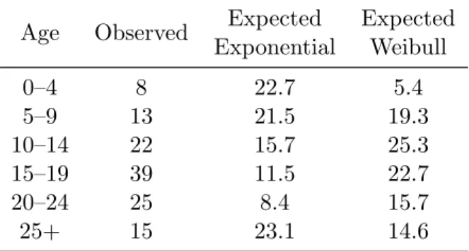
We obtain then X2 = 17.9 for the Weibull model, and X2 = 92.2 for the exponential distribution. The latter produces a p-value on the order of 10−18, but the former has a p-value around 0.0013. Thus, while the data could not possibly have come from an exponential distribution, or anything like it, the Weibull distribution, while unlikely to have produced exactly these data, is a plausible candidate.
Age Observed Expected Expected Exponential Weibull 0–4 8 22.7 5.4 5–9 13 21.5 19.3 10–14 22 15.7 25.3 15–19 39 11.5 22.7 20–24 25 8.4 15.7 25+ 15 23.1 14.6
Table 1.2: χ2 computation for fitting tyrannosaur data.
1.3
Overview of the course
Why do we need special statistical methods for lifetime data? Some reasons are:
• Large samplesOther models, such as single-decrement models with time-varying tran-sition rates, may be closer to the truth. We may have more elaborate multivariate para-metric models for the transition rates, but they are unlikely to be precisely true. The problem then is that the parametric families will eventually be rejected, once the sample size is large enough — and since we may be concerned with statistical surveys of, for example, the entire population of the UK, the sample sizes will be very large indeed. Nonparametric or semiparametric methods will be better able to let the data speak for themselves.
• Small samples While nonparametric models allow the data to speak for themselves, sometimes we would prefer that they be somewhat muffled. When the number of ob-served deaths is small — which can be the case, even in a very large data set, when considering advanced ages, above 90, and certainly above 100, because of the small num-ber of individuals who survive to be at risk, but also in children, because of the very low mortality rate — the estimates are less reliable, being subject to substantial random noise. Also, the mortality pattern changes over time, and we are often interested in fu-ture mortality, but only have historical data. A non-parametric estimate that precisely reflects the data at hand may reflect less well the underlying processes, and be ill-suited to projection into the future. Graduation (smoothing) and extrapolation methods have been developed to address these issues.
• Incomplete observationsSome observations will be incomplete. We may not know the exact time of a death, but only that it occurred before a given time, or after a given time, or between two known times, a phenomenon called “censoring”. (When we are informed only of the year of a death, but not the day or time, this is a kind of censoring. Or we may have observed only a sample of the population, with the sample being not entirely random, but chosen according to being alive at a certain date, or having died before a certain date, a phenomenon known as “truncation”. We need special techniques to make use of these partial observations.) Since we are observing times, subjects who break off a study midway through provide partial information in a clearly structured way.
• Successive eventsA key fact about time is its sequence. A patient is infected, develops symptoms, has a diagnosis, a treatment, is cured or relapses, at some point dies. Some
or all of these events may be considered as a progression, and we may want to model the sequence of random times. Some care is needed to carry out joint maximum likelihood estimation of all transition rates in the model, from one or several individuals observed. This can be combined with time-varying transition rates.
• Comparing lifetime distributionsWe may wish to compare the lifetime distributions of different groups (e.g., smokers and nonsmokers; those receiving a traditional cholesterol medication and those receiving the new drug) or the effect of a continuous parameter (e.g., weight) on the lifetime distribution.
• Changing rates Mortality rates are not static in time, creating disjunction between period measures — looking at a cross-section of the population by age as it exists at a given time — and cohortmeasures — looking at a group of individuals born at a given time, and following them through life.
Lifetime distributions
All the stochastic models in this course will be within the class of discrete state-space Markov processes which may be time inhomogeneous. We will not be using the general form of these models, but will be simplifying and specialising them substantially. What unifies this course is the nature of the questions we will be asking. In the standard theory of Markov processes, we focus early on stationary processes. Our models will not be stationary, because they have absorbing states. The key questions will concern the absorbing states: When the process is absorbed (the “lifetime”), and, in some models, which state absorbs it.
We need to be careful to distinguish between representations of the population and repre-sentations of the individual. In the present context, the Markov process always represents an individual. The population consists of some number of independently running copies of the basic Markov process. In simple cases — for instance, exponential mortality — the population-level process (total population at timet) will also be a Markov process, a “pure-death” chain. This raises the complication that there are usually two different kinds of time running: The “internal” time of the individual process, which usually represents age in some way, and calen-dar time. The full implications of these interacting time-frames — also called the cohort and the period perspective — are a major topic in demography, and we will only touch on them in this course.
2.1
Survival function and hazard rate (force of mortality)
As discussed in chapter 1, the simplest lifetime model is the single-decrement model: The in-dividual is alive for some length of time L, at the end of which he/she becomes dead. This is a homogeneous Markov process if and only if L has an exponential distribution. In general, we may describe a lifetime distribution — which is simply the distribution of a nonnegative random variable — in several different ways:
cdf F(t) =PL≤t ;
survival function S(t) = ¯F(t) = 1−F(t) =PL > t ; density function f(t) =dF/dt;
hazard rate λ(t) =f(t)/F¯(t)
The hazard rate is also called mortality rate in survival contexts. The traditional name in demography is force of mortality. This may be thought of as the instantaneous rate of dying per unit time, conditioned on having already survived.s The exponential distribution with pa-rameterλ∈(0,∞) is given by
cdf F(t) = 1−e−λt; survival function F¯(t) =e−λt;
density function f(t) =λe−λt; hazard rate λ(t) =λ.
Thus, the exponential is the distribution with constant force of mortality, which is a formal statement of the “memoryless” property.
2.2
Residual lifetimes
Assume that there is an overall lifetime distribution, and every individual born has a random lifetime according to this distribution. Then, if we observe sombody now agedx, and we denote his residual lifetimeT −x byTx, then we have
¯ FTx(t) = ¯FT−x|T >x(t) = ¯ FT(x+t) ¯ FT(x) , fTx(t) =fT−x|T >x(t) = fT(x+t) ¯ FT(x) , t≥0. (1) So, any distribution of a full lifetime T is naturally associated with a family of conditional distributions ofT given T > x.
2.3
Force of mortality
We now look more closely at the hazard rate, which may be defined as
hT(t) =µt= lim ε↓0 1 εP(T ≤t+ε|T > t) = limε↓0 1 εP(t < T ≤t+ε) P(T > t) = fT(t) ¯ FT(t) . (2)
The density fT(t) is the (unconditional) infinitesimal probability to die at age t. The hazard
rate hT(t) is the (conditional) infinitesimal probability to die at age tof an individual known
to be alive at aget. It may seem that the hazard rate is a more complicated quantity than the density, but it is very well suited to modelling mortality. Whereas the density has to integrate to one and the distribution function (survival function) has boundary values 0 and 1, the force of mortality has no constraints, other than being nonnegative — though if “death” is certain the force of mortality has to integrate to infinity. Also, we can read its definition as a differential equation and solve
¯ FT0(t) =−µtF¯T(t), F¯(0) = 1 ⇒ F¯T(t) = exp − Z t 0 µsds , t≥0. (3) We can now express the distribution ofTx as
¯ FTx(t) = ¯ FT(x+t) ¯ FT(x) = exp − Z x+t x µsds = exp − Z t 0 µx+rdr , t≥0. (4)
Note that this implies thathTx(t) =hT(x+t), so it is really associated with agex+tonly, not
with initial agex nor with timetafter initial age. Also note that, given a measurable function
µ: [0,∞) → R, ¯FTx(0) = 1 always holds, ¯FTx decreasing if and only if µ ≥0. ¯FTx(∞) = 0 if
and only if R0∞µtdt=∞. This leaves a lot of modelling freedom via the force of mortality.
Densities can now be obtained from the definition of the force of mortality (and consistency) asfTx(t) =µt+xF¯Tx(t).
2.4
Defining mortality laws from hazards
We are now in the position to model mortality laws via their force of mortality. Clearly, the Exp(λ) distribution has a constant hazard rate µt ≡λ, and the uniform distribution on [0, ω]
has a hazard rate
hT(t) =
1
ω−t, 0≤t < ω. (5)
Note that hereRω
0 hT(t)dt=∞ squares with ¯FT(ω) = 0 and forces the maximal ageω. This is
a general phenomenon: distributions with compact support have a divergent force of mortality at the supremum of their support, and the singularity is not integrable.
The Gompertz distribution is given by µt =Beθt. More generally, Makeham’s law is given
by
µt=A+Beθt, F¯Tx(t) = exp
n
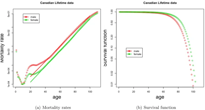
−At−meθ(x+t)−eθxo, x≥0, t≥0, (6) for parametersA >0,B >0,θ >0;m=B/θ. Note that mortality grows exponentially. Ifθis big enough, the effect is very close to introducing a maximal ageω, as the survival probabilities decrease very quickly. There are other parameterisations for this family of distributions. The Gompertz distribution is named for British actuary Benjamin Gompertz, who in 1825 first published his discovery [Gom25] that human mortality rates over the middle part of life seemed to double at constant age intervals. It is unusual, among empirical discoveries, for having been confirmed rather than refuted as data have improved and conditions changed, and it (or Makeham’s modification) serves as a standard model for mortality rates not only in humans, but in a wide variety of organisms. As an example, see Figure2.1, which shows Canadian mortality rates from life tables produced by Statistics Canada (available at http://www.statcan.ca: 80/english/freepub/84-537-XIE/tables.htm). Notice how close to a perfect line the mid-life mortality rates for both males and females is, when plotted on a logarithmic scale, showing that the Gompertz model is a very good fit.
Figure 2.1(b) shows the corresponding survival curves. It is worth recognising how much more informative the mortality rates are. in Figure 2.1(a) we see that male mortality is reg-ularly higher than female mortality at all ages (and by a fairly constant ratio), we see several phases of mortality — early decline, jump in adolescence, then steady increase through midlife, and deceleration in extreme old age — whereas Figure 2.1(b)shows us only that mortality is accelerating overall, and that males have accumulated higher mortality by late life.
TheWeibull distribution suggests a polynomial rather than exponential growth of mortality
µt=ktn, F¯Tx(t) = exp − k n+ 1 (x+t) n+1−xn+1 , x≥0, t≥0, (7) for rate parameterk >0 and exponentn >0. The Weibull model is commonly used in engineer-ing contexts to represent the failure-time distribution for machines. The Weibull distribution arises naturally as the lifespan of a machine withn redundant components, each of which has
0 20 40 60 80 100 1e-04 5e-04 5e-03 5e-02 5e-01
Canadian Lifetime data
age
Mortality rate
male female
(a) Mortality rates
0 20 40 60 80 100 0.01 0.02 0.05 0.10 0.20 0.50 1.00
Canadian Lifetime data
age
Survival function
male female
(b) Survival function
Figure 2.1: Canadian mortality data, 1995–7.
constant failure rate, such that the machine fails only when all components have failed. Later in the course we will discuss how to fit Weibull and Gompertz models to data.
Another class of distributions is obtained by replacing the parameter λ in the exponen-tial distribution by a (discrete or continuous) random variable M. Then the specification of exponential conditional densities
fT|M=λ(t) =λe−λt (8)
determines the unconditional density of T as
fT(t) = Z ∞ 0 fT ,M(t, λ)dλ= Z ∞ 0 λe−λtfM(λ)dλ or fT(t) = X λ>0 λe−λtP(M =λ). (9) Various special cases of exponential mixtures and other extensions of the exponential distribu-tion have been suggested in a life insurance context. Some of these will be presented later.
E.g., for M ∼Geom(p), i.e.P(M =k) =pk−1(1−p), k≥1, we obtain ¯ FT(t) = Z ∞ t fT(s)ds= Z ∞ t ∞ X k=1 fT|M=k(s)pk−1(1−p)ds = ∞ X k=1 Z ∞ t ke−ktpk−1(1−p)ds= (1−p)e −t 1−pe−t
and one easily deduces
fT(t) =
(1−p)e−t
(1−pe−t)2, t≥0.
The corresponding hazard rate is
hT(t) = fT(t) ¯ FT(t) = 1 1−pe−t,
2.5
Curtate lifespan
We have implicitly assumed that the lifetime distribution is continuous. However, we can always pass from a continuous random variableT on [0,∞) to a discrete random variable K = [T], its integer part, on N. IfT models a lifetime, thenK is called the associated curtate lifetime.
2.6
Single decrement model
The exponential model may also be represented as a Markov process. Let S = {0,1} be our state space, with interpretation 0=‘alive’ and 1=‘dead’, and consider theQ-matrix
Q= −µ µ 0 0 . (10)
Then a continuous-time Markov chain X = (Xt)t≥0 with X0 = 0 and Q-matrix Q will have a
holding timeT ∼exp(µ) in state 0 before a transition to 1, where it is absorbed, i.e.
Xt=
0 if 0≤t < T
1 ift≥T . (11)
The transition matrix is
Pt=etQ= e−µt 1−e−µt 0 1 .
It seems that this is an overly elaborate description of a simple model (diagrammed in Figure
2.2), but this viewpoint will be useful for generalisations. Also, the ‘rate parameter’ µ has a more concrete meaning, and the lack of memory property of the exponential distribution is also reflected in the Markov property: given that the chain is still in state 0 at time t (i.e. given
T > t), the residual holding time (i.e. T −t) has conditional distribution Exp(µ).
Alive
μ
Dead
Figure 2.2: The single-decrement model.
This model may be generalised by allowing the transition rateµto become an age-dependent rate function t 7→ µ(t). This may be seen as a very special kind of inhomogeneous Markov process, or as a special kind of renewal process (one with only one transition). The general two-state model with transient two-state ‘alive’ and absorbing two-state ‘dead’, is called the ‘single-decrement model’.
2.7
Mortality laws: Simple or Complex? Parametric or
Non-parametric?
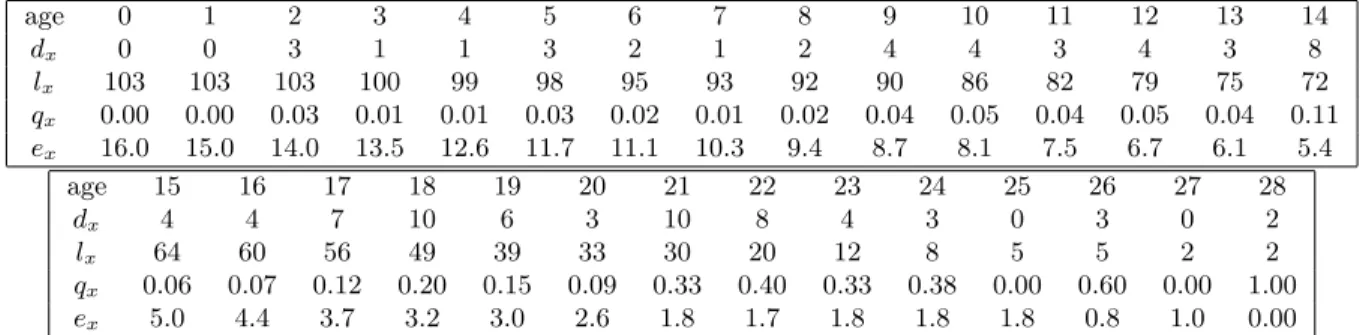
Consider the data for Albertosaurus sarcophagus in Table 1.1. We see here the estimated ages at death for 22 members of this species. Let us assume, for the sake of discussion, that these estimates are correct, and that our skeleton collection represents a simple random sample of all Albertosaurs that ever lived. If we assume that there was a large population of these dinosaurs, and that they died independently (and not, say, in a Cretaceous suicide pact), then these are 22 independent samplesT1, . . . , T22of a random variableT whose distribution we would like to know. Consider the probabilities
qx :=Px≤T < x+ 1 .
Then the number of individuals observed to have curtate lifespan x has binomial distribution
Bin(22, qx). The MLE for a binomial probability is just the na¨ıve estimate ˆqx= # successes/# trials
(where a “success”, in this case, is a death in the age interval under consideration). To compute ˆ
q2, then, we observe that there were 22 Albertosaurs from our sample still alive on their 22 birthdays, of which one unfortunate met its maker in the following year: ˆq2 = 1/22≈0.046.As for ˆq3, on the other hand, there were 21 Albertosaurs observed alive on their third birthdays,
and all of them arrived safely at their fourth, making ˆq3 = 0/21. This leads us to the peculiar
conclusion that our best estimate for the probability of an albertosaur dying in its third year is 0.046, but that the probability drops to 0 in its fourth year, then becomes nonzero again in the fifth year, and so on. This violates our intuition that mortality rates should be fairly smooth as a function of age. This problem becomes even more extreme when we consider continuous lifetime models. With no constraints, the optimal estimator for the mortality distribution would put all the mass on just those moments when deaths were observed in the sample, and no mass elsewhere — in other words, infinite hazard rate at a finite set of points at which deaths have been observed, and 0 everywhere else.
As we see from Figure 1.1, the mortality distribution for the tyrannosaurs becomes much smoother and less erratic when we use larger bins for the histogram. This is no surprise, since we are then sampling from a larger baseline, leading to less random fluctuation. The simplest way to impose our intuition of regularity upon the estimators is to increase the time-step and reduce the number of parameters to estimate. An extreme version of this, of course, is to impose a parametric model with a small number of parameters. This is part of the standard tradeoff in statistics: a free, nonparametric model is sensitive to random fluctuations, but constraining the model imposes preconceived notions onto the data.
Notation: When the hazard rate µx is being assumed constant over each year of life, the
continuous mortality rate has been reduced to a discrete set of parameters. What do we call these parameters? By convention, the value of µ that is in effect for all ages in [x, x+ 1) is identified with just one age, namelyµx+1
Life Tables
Reading: Gerber Sections 2.4-2.5, CT4 Units 5-2, 6, 10-1 Further reading: Cox-Oakes Sections 4.1-4.4, Gerber Sections 11.1-11.5
Life tables represent a discretised form of the hazard function for a population, often together with raw mortality data. Apart from an aggregate table subsuming the whole population (of the UK, say), such tables exist for various groups of people characterized by their sex, smoking habits, job type, insurance level etc. This immediately raises interesting questions concerning the interdependence of such tables, but we focus here on some fundamental issues, which are already present for the single aggregate table.
We begin with a na¨ıve, empirical approach. In Table 3.2 we see a life table for men in the UK, in the years 1990–2, as provided by the Office of National Statistics. In the column labelled
Ex we see the number of years “exposed to risk” in age-class x. Since everyone alive is at risk
of dying, this should be exactly the sum of the number of individuals alive in the age class in years 1990, 1991, and 1992. The 1991 number is obtained from the census of that year, and the other two years are estimated. The column dx shows the number of men of the given age
known to have died during this three-year period. The final column ismx :=dx/Ex.
Again, this is an empirical fact, but we find ourselves in a quandary when we try to interpret it. What ismx? If the number of deaths is reasonably stable from year to year, thenmxshould
be close to the fraction of men agedx who died each year. How close? The number of men at risk changes constantly, with each birthday, each death, each immigration or emigration. We sense intuitively that the effect of these changes would be small, but how small? And what would we do to compensate for this in a smaller population, where the effects are not negligible? How do we make projections about future states of the population?
3.1
Notation for life tables
qx Probability that individual agedx dies before reaching agex+ 1
px Probability that individual agedx survives to agex+ 1
tqx Probability that individual agedx dies before reaching agex+t tpx Probability that individual agedx survives to agex+t
lx Number of people who survive to age x. Note: This is based
on starting with a fixed number l0 of lives, called theRadix;
most commonly, for human populations the radix is 100,000
dx Number of individuals who die agedx (from the standard population) tmx Mortality rate between exact agex and exact agex+t
ex Remaining life expectancy at age x
Note the following relationships:
dx =lx−lx+1; lx+1 =lxpx =lx(1−qx); tpx = t−1 Y i=0 px+i
The quantitiesqxmay be thought of as the discrete analogue of the mortality rate — we will
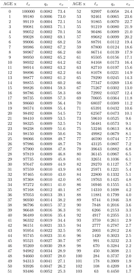
call it thediscrete mortality rateordiscrete hazard function— since it describes the probability of dying in the next unit of time, given survival up to agex. In Table3.1we show the life table computed from the raw data of Table3.2. (It differs slightly from the official table, because the official table added some slight corrections. The differences are on the order of 1% in qx, and
much smaller in lx.) The life table represents the effect of mortality on a nominal population
starting with size l0 called the Radix, and commonly fixed at 100,000 for large-population life
tables. Imagine 100,000 identical individuals — a cohort — born on 1 January, 1900. In the column qx we give the estimates for the probability of an individual who is alive on his x
birthday dying in the next year, before his x+ 1 birthday. (We discuss these estimates later in the chapter.) Thus, we estimate that 820 of the 100,000 will die before their first birthday. The survivingl1 = 99,180 on 1 January, 1901, face a mortality probability of 0.00062 in their next year, so that we expect 61 of them to die before their second birthday. Thus l2 = 99119.
And so it goes. The final column of this table, labelled ex, gives remaining life expectancy; we
will discuss this in section??.
3.2
Continuous and discrete models
3.2.1 General considerations
The first decision that needs to be made in setting up a lifetime model is whether to model lifetimes as continuous or discrete random variables. On first consideration, the discrete ap-proach may seem to recommend itself: after all, we are commonly concerned with mortality data given in whole years or, if not years, then whole numbers of months, weeks, or days. Real measurements are inevitably discrete multiples of some minimal unit of precision. In fact, though, discrete models for measured quantities are problematic because
• They tie the analysis to one unit of measurement. If you start by measuring lifespans in years, and restrict the model accordingly you have no way of even posing a question about, for instance, the effect of shifting the reporting date within the year.
• Discrete methods are comfortable only when the numbers are small, whereas moving down to the smallest measurable unit turns the measurements into large whole numbers. Once you start measuring an average human lifespan as 30000 days (more or less), real numbers become easier to work with, as integrals are easier than sums.
• It is relatively straightforward to embed discrete measures within a continuous-time model, by considering the integer part of the continuous random lifetime, called the curtate lifetimein actuarial terminology.
(Compare this to the suggestion once made by the physicist Enrico Fermi, that lecturers might take their listeners’ investment of time more seriously if they thought of the 50-minute span of a lecture as a “microcentury”.) The discrete model, it is pointed out by A. S. Macdonald in [Mac96] (and rewritten in [CT406, Unit 9]), “is not so easily generalised to settings with more than one decrement. Even the simplest case of two decrements gives rise to difficult problems,” and involves the unnecessary complication of estimating an Initial Exposed To Risk. We will generally treat the continuous model as the fundamental object, and treat the discrete data as coarse representations of an underlying continuous lifetime. However, looking beyond the actuarial setting, there are models which really do not have an underlying continuous time parameter. For instance, in studies of human fertility, time is measured in menstrual cycles, and there simply are no intermediate chances to have the event occur.
3.2.2 Are life tables continuous or discrete?
The standard approach to life tables mixes the continuous and discrete, in sometimes confusing ways. The data upon which life tables are based are measured in discrete units, but in most applications we assume that the risk is actually continuous. If we were to observe a fixed number of individuals for exactly one year, and count the number of deaths at the end of the year, and if the number of deaths during the year were a small fraction of the total number at risk, it would hardly matter whether we chose a discrete or continuous model. As we discuss in chapter5.3, the distinction becomes significant to the extent that the number of individuals at risk changes substantially over a single time unit; then we need to distinguish amongInitial Exposed To Risk,Central Exposed To Risk, and thecensus approximation(see chapter5.3).
The connection between discrete and continuous laws is fairly straightforward, at least in one direction. Suppose T is a lifetime with hazard rate µx at age x, and qx is the probability
of dying on or after birthdayx, and before thex+ 1 birthday. Then
tqx=e−
Rx+t
x µsds.
Another way of putting this is to say that the discrete model may be embedded in the continuous model, by considering the discrete random variableK = [T], called the associated
curtate lifetime. The remainder (fractional part) S = T −K = {T} can often be treated separately in a simplified way (see below). Clearly, the probability mass function ofK on Nis
given by P(K =n) =P(n≤T < n+ 1) = Z n+1 n fT(t)dt= ¯FT(n)−F¯T(n+ 1) = exp − Z n 0 µT(t)dt 1−exp − Z n+1 n µT(t)dt
and if we denote the one-year death probabilities (discrete hazard function) by
qk =P(K =k|K≥k) = P(K =k) P(K ≥k) = 1 −exp − Z k+1 k µT(t)dt
andpk= 1−qk,k∈N, we obtain the probability of success afternindependent Bernoulli trials with varying success probabilitiesqk:
P(K =n) =p0. . . pn−1qn.
Note thatqkonly depends on the hazard rate between ages kandk+ 1. As a consequence, for
Kx= [Tx]
P(Kx =n) =px. . . px+n−1qx+n
are also easily represented in terms of (qk)k∈N.
3.3
Interpolation for non-integer ages
Suppose now that we have modeled the curtate lifetimeK. The fractional partS of the lifetime is a random variable on the interval [0,1], commonly modeled in one of the following ways: Constant force of mortality µ(x) is constant on the interval [k, k+1), and is calledµT(k+12),
or sometimesµk+1
2 when T is clear from the context. Then 1qk= 1−e
−µ
k+ 12; µ
k+12 =−lnpk.
S has the distribution of an exponential random variable conditioned on S <1, so it has density f(s) =µk+1 2 e−µk+ 1 2 s 1−e−µk+ 12 .
This assumption thus implies decreasing density of the lifetime through the interval. We also have, for 0≤s≤1, andk an integer,
spk =P(T > k+s|T > k) = exp − Z k+s k µtdt = expn−sµk+1 2 o = (1−qk)s.
Note thatK and S are not independent, under this assumption. Uniform IfS is uniform on [0,1), this implies that for s∈[0,1),
fT(k+s) = ( ¯FT(k)−F¯T(k+ 1)) = ¯FT(k)qk, sqk=s·1qk, ¯ FT(k+s) = ¯FT(k) 1−sqk , µT(k+s) = fT(k+s) ¯ FT(k+s) = qk 1−sqk .
So this assumption implies that the force of mortality is increasing over the time unit. Note that µ is discontinuous at (some if not all) integer times unless q0 = α = 1/n and
qx+1 =qx/(1−qx), i.e. qk = 1−αkα,k = 1, . . . , n−1, with ω =n maximal age. Usually,
one accepts discontinuities.
Balducci 1−tqk+t = (1−t)qk for t∈ [0,1), so that the probability of death in the remaining
time 1−t, having survived tok+t, is the product of the time left and the probability of death in [k, k+ 1). There is a trivial identity that the probability of surving 1 time unit from timekis the probability of survivingttime units from timek, times the probability of surviving 1−ttime units from timek+t. Thus
qk = 1−(1−tqk)·(1−1−tqk+t) = 1−(1−tqk)·(1−(1−t)qk), so that tqk= 1− 1−qk 1−(1−t)qk ,
This implies that ¯ FT(k+t) = ¯FT(k)P T > k+tT > k = ¯FT(k) 1−qk 1−qk+tqk fT(k+t) = d dt ¯ FT(k+t) = ¯ FT(k)qk(1−qk) (1−qk+tqk)2 , µT(k+t) = fT(k+t) ¯ FT(k+t) = qk 1−qk+tqk
So this assumption implies that the force of mortality is decreasing over the time unit. Once we have made one of these assumptions, we can reconstruct the full distribution of a lifetime T from the entries (qx)x∈N of a life table. When the force of mortality is small, these
different assumptions are all equivalent toµk+1
2 =qk. Notice again that the choice of a
measure-ment unit for discretisation implies a certain level of smoothing, in continuous nonparametric life table computations. Taking the evidence at face value, we would have to say that we have observed zero mortality rate, except at the instants at which deaths were observed, where mor-tality jumps to∞. Of course, we average over a period of time, either by imposing the constraint that mortality rates be step functions, constant over a single measurement unit (or multiple units, if we wish to impose additional smoothing, usually because the number of observations is small).
Moving in the other direction is not so straightforward. The continuous model cannot be embedded in the discrete model, for obvious reasons: within the framework of the discrete model, there is no such thing as a death midway through a time period. Traditionally, when the discrete nature of lifetable data has been in the foreground, a model of the fractional part, such as one of those listed above, has been adjoined to the model. As described in section3.2.1, this approach quickly collapses under the weight of unnecessary complications, which is why we will always treat the continuous lifetime as the fundamental object, except when the lifetime truly is measured only in discrete units.
3.4
Crude estimation of life tables – discrete method
Since their invention in the 17th century, the basic methodology for life table has been to collect (from the church registry or whoever kept records of births and deaths) lifetimes, truncate to integer lifetimes, count the numbers dx of deaths between ages x and x+ 1, relate this to the
numbers `x alive at age x, and use ˆqx(0) = dx/`x, or similar quantities as an estimate for the
one-year death probabilityqx.
In our model, the deaths are Bernoulli events with probability qx, so we know that the
Maximum Likelihood Estimator for qx is ˆq
(0)
x = # successes/# trials = dx/`x for n = `0
independently observed curtate lifetimesk1, . . . , kn, observed from random variables with
com-mon probability mass function (m(x))x∈N parameterized by (qx)x∈N. If we denote m(x) =
(1−q0). . .(1−qx−1)qx, the likelihood is n Y i=1 m(k(i)) = Y x∈N (m(x))dx = Y x∈N (1−qx)`x−dxqdxx , (1)
where only max{k1, . . . , kn}+ 1 factors in the infinite product differ from 1, and
dx=dx(k1, . . . , kn) = # n 1≤i≤n:k(i)=x o , `x =`x(k1, . . . , kn) = # n 1≤i≤n:k(i)≥xo.
This product is maximized when its factors are maximal (the xth factor only depending on parameter qx). An elementary differentiation shows that q 7→ (1−q)`−dqd is maximal for
ˆ q=d/`, so that ˆ qx(0)= ˆq(0)x (k1, . . . , kn) = dx(k1, . . . , kn) `x(k1, . . . , kn) , 0≤x≤max{k1, . . . , kn}.
Note that for x = max{k1, . . . , kn}, we have ˆqx(0) = 1, so no survival beyond the highest age
observed is possible under the maximum likelihood parameters, so that (ˆq(0))0≤x≤max{k1,...,kn}
specifies a unique distribution. (Varying the unspecified parametersqx,x > max{k1, . . . , kn},
has no effect.)
3.5
Crude life table estimation – continuous method
Alternatively, we can take a maximum likelihood approach on the continuous lifetimes, and obtain a different estimator. Assume that you observe n = `0 independent lives t1, . . . , tn.
Then the likelihood function is
n Y i=1 fT(ti) = n Y i=1 µtiexp − Z ti 0 µsds (2) Now assume that the force of mortality µs is constant on [x, x+ 1), x ∈ N and denote these values by µx+1 2 = −ln(px) remember px= exp − Z x+1 x µsds . (3)
Then, the likelihood takes the form Y x∈N µdxx+1 2 exp n −µx+1 2 ˜ `x o (4) where only max{t1, . . . , tn}+ 1 factors in the infinite product differ from 1, and
dx=dx(t1, . . . , tn) = #{1≤i≤n: [ti] =x}, ˜ `x= ˜`x(t1, . . . , tn) = n X i=1 Z x+1 x 1{ti>s}ds. ˜
`x is called thetotal exposed to risk.
The quantities µx+1 2, x
∈ N, are the parameters, and we can maximise the product by maximising each of the factors. An elementary differentiation shows that µ 7→ µde−µ` has a
unique maximum at ˆµ=d/`, so that ˆ µx+1 2 = ˆµx+ 1 2(t1, . . . , tn) = dx(t1, . . . , tn) ˜ `x(t1, . . . , tn) , 0≤x≤max{t1, . . . , tn}.
Since maximum likelihood estimators are invariant under reparameterisation (the range of the likelihood function remains the same, and the unique parameter where the maximum is obtained can be traced through the reparameterisation), we obtain
ˆ qx= ˆqx(t1, . . . , tn) = 1−pˆx = 1−exp n −ˆµx+1 2 o = 1−exp −dx(t1, . . . , tn) ˜ `x(t1, . . . , tn) . (5)
For smalldx/`˜x, this is close to dx/`˜x, and therefore also close to dx/`x.
Note that under ˆqx, x ∈ N, there is a positive survival probability beyond the highest observed age, and the maximum likelihood method does not fully specify a lifetime distribution, leaving free choice beyond the highest observed age.
3.6
Comparing continuous and discrete methods
There appears to be a contradiction between the discrete life-table estimation of section3.4and the continuous life-table estimation of section 3.5. While the models are different, there are questions to which both offer an answer, and the answers are different. In the discrete model, we estimate
PT < x+ 1T ≥x =qx≈qˆx=
dx
`x
.
The continuous model suggests that we estimate the same quantity by PT < x+ 1T ≥x = 1−e −µx+ 1 2 ≈1−e −µˆx+ 1 2 = 1−e−dx/`x˜ ≤ dx ˜ `x . (6)
If we take `x as a substitute for ˜`x, then, the continuous model gives a strictly smaller
answer, unlessdx = 0. Why is that? The difference here is that the continuous model presumes
if we make the estimate ˜`x ≈`x−dx/2 (so presuming that those who died lived on average half
a year), substituting the Taylor series expansion into (6) shows that in the continuous model PT < x+ 1T ≥x = dx `x−dx/2 − dx 2(`x−dx/2)2 +o dx `x−dx/2 3 = dx `x +o dx `x−dx/2 3 .
That is, when the mortality fractiondx/`x is small, the estimates agree up to second order in
dx/`x.
3.7
An example: Fractional lifetimes can matter
Imagine an insurance company that insures valuable pieces of construction machinery, which we will call piddledonks. For safety reasons, piddledonks cannot be used more than 3 years, but they may fail before that time. The company has records on 1000 of these machines, summarised in Table 3.3. That is, 100 failed in their first year (age 0), 400 in the second year, and 400 in the third year of operation. The last column shows the estimated failure probabilities.
Table 3.3: Life table for piddledonks. agex lx dx qx
0 1000 100 0.10 1 900 400 0.44 2 500 400 0.80
Suppose the company sells insurance policies that pay £1000 when a piddledonk fails. The fair price for such a contract will be£100 for a new-built piddledonk. (That is, the price equal to the expected value of the contract; obviously, a company that wants to cover its costs and even turn a profit needs to sell its insurance somewhat above the nominal fair price.) It will be
£444 for a piddledonk on its first birthday, and £800 for a piddledonk on its second birthday. Suppose, though, someone comes with a piddledonk that is 18 months old, and wishes to buy insurance for the next half year. What would be the fair price?
We have no data on when in the year failure occurs. It is possible, in principle, that piddledonks fail only on their birthdays; if they survive that day, they’re good for the rest of the year. In that case, the insurance could be free, since the probability of a failure in the second half year is 0. This seems implausible, though. Suppose we adopt the constant-hazard model. Calling the constant hazardµ, we see thatp1 =e−µ, and
p1 =0.5p1·0.5p1.5. (7) Thus, 0.5p1.5=0.5p1=e−µ/2 = √ p1 = p 1−q1= √ .555 = 0.745,
and 0.5q1.5 = 0.255, and the fair price for the half year of insurance is £255. Suppose, on the
other hand, we adopt the uniform model forS. We still have (7), but now
0.5p1 = 1−0.5q1= 1−
1 21q1,
so that 0.5p1.5 = p1 1−1 2 1q1 = 0.555 .778 = 0.713, implying that the fair price for this insurance would be £287.
AGE x Ex dx mx×105 0 1066867 8779 823 1 1059343 661 62 2 1054256 403 38 3 1047298 319 30 4 1037973 251 24 5 1022032 229 22 6 1003486 201 20 7 989008 186 19 8 976049 180 18 9 981422 180 18 10 988020 179 18 11 984778 179 18 12 950853 185 19 13 909437 212 23 14 891556 259 29 15 913423 366 40 16 954339 496 52 17 1002077 758 76 18 1057508 922 87 19 1124668 930 83 20 1163581 979 84 21 1195366 1030 86 22 1210521 1073 89 23 1238979 1105 89 24 1263313 1083 86 25 1296300 1068 82 26 1313794 1145 87 27 1311662 1090 83 28 1291017 1110 86 29 1259644 1129 90 30 1219278 1101 90 31 1176120 1144 97 32 1135091 1128 99 33 1103162 1095 99 34 1071474 1142 107 35 1035587 1218 118 36 1017422 1291 127 37 1010544 1399 138 38 1006929 1536 153 39 1006500 1660 165 40 1016727 1662 163 41 1046632 1967 188 42 1092927 2240 205 43 1167798 2543 218 44 1134652 2656 234 45 1071729 2836 265 46 974301 2930 301 47 955329 3251 340 48 914107 3354 367 49 848419 3486 411 50 815653 3836 470 51 811134 4251 524 AGE x Ex dx mx×105 52 827414 4781 578 53 822603 5324 647 54 810731 5723 706 55 794930 6411 806 56 775350 6925 893 57 759747 7592 999 58 755475 8477 1122 59 761913 9484 1245 60 764497 10735 1404 61 753706 11880 1576 62 736868 12871 1747 63 725679 14463 1993 64 721743 16094 2230 65 713576 17704 2481 66 700666 19097 2726 67 681977 20930 3069 68 676972 22507 3325 69 678157 25127 3705 70 684764 27159 3966 71 600343 26508 4415 72 504808 24443 4842 73 422817 22792 5391 74 422480 24921 5899 75 431321 27286 6326 76 422822 29712 7027 77 399257 30856 7728 78 365168 30744 8419 79 328386 30334 9237 80 293014 29788 10166 81 260517 28483 10933 82 229149 27399 11957 83 197322 25697 13023 84 165896 23717 14296 85 136103 20930 15378 86 110565 18689 16903 87 87989 16370 18605 88 68443 13571 19828 89 52151 11284 21637 90 40257 9061 22508 91 29000 7032 24248 92 20124 5405 26858 93 13406 4057 30263 94 9392 3069 32677 95 6446 2219 34424 96 4384 1578 35995 97 2795 1091 39034 98 1761 701 39807 99 1059 489 46176 100 624 292 46795 101 359 178 49582 102 216 118 54630 103 107 63 58879
Table 3.1: Male mortality data for England and Wales, 1990–2. From [Fox97] (available online athttp://www.statistics.gov.uk/StatBase/Product.asp?vlnk=333).
AGE x `x qx ex 0 100000 0.0082 73.4 1 99180 0.0006 73.0 2 99119 0.0004 72.1 3 99081 0.0003 71.1 4 99052 0.0002 70.1 5 99028 0.0002 69.1 6 99006 0.0002 68.2 7 98986 0.0002 67.2 8 98967 0.0002 66.2 9 98950 0.0002 65.2 10 98932 0.0002 64.2 11 98914 0.0002 63.2 12 98896 0.0002 62.2 13 98877 0.0002 61.2 14 98855 0.0003 60.2 15 98826 0.0004 59.3 16 98786 0.0005 58.3 17 98735 0.0008 57.3 18 98660 0.0009 56.4 19 98574 0.0008 55.4 20 98492 0.0008 54.5 21 98410 0.0009 53.5 22 98325 0.0009 52.5 23 98238 0.0009 51.6 24 98150 0.0009 50.6 25 98066 0.0008 49.7 26 97986 0.0009 48.7 27 97900 0.0008 47.8 28 97819 0.0009 46.8 29 97735 0.0009 45.8 30 97647 0.0009 44.9 31 97559 0.0010 43.9 32 97465 0.0010 43.0 33 97368 0.0010 42.0 34 97272 0.0011 41.0 35 97168 0.0012 40.1 36 97053 0.0013 39.1 37 96930 0.0014 38.2 38 96796 0.0015 37.2 39 96648 0.0016 36.3 40 96489 0.0016 35.4 41 96332 0.0019 34.4 42 96151 0.0021 33.5 43 95954 0.0022 32.5 44 95745 0.0023 31.6 45 95521 0.0027 30.7 46 95269 0.0030 29.8 47 94982 0.0034 28.9 48 94660 0.0037 28.0 49 94313 0.0041 27.1 50 93926 0.0047 26.2 51 93486 0.0052 25.3 AGE x `x qx ex 52 92997 0.0058 24.4 53 92461 0.0065 23.6 54 91865 0.0070 22.7 55 91219 0.0080 21.9 56 90486 0.0089 21.0 57 89682 0.0099 20.2 58 88791 0.0112 19.4 59 87800 0.0124 18.6 60 86714 0.0139 17.9 61 85505 0.0156 17.1 62 84168 0.0173 16.4 63 82710 0.0197 15.6 64 81078 0.0221 14.9 65 79290 0.0245 14.3 66 77347 0.0269 13.6 67 75267 0.0302 13.0 68 72992 0.0327 12.4 69 70605 0.0364 11.8 70 68037 0.0389 11.2 71 65391 0.0432 10.6 72 62567 0.0473 10.1 73 59610 0.0525 9.6 74 56481 0.0573 9.1 75 53246 0.0613 8.6 76 49982 0.0679 8.1 77 46590 0.0744 7.7 78 43125 0.0807 7.2 79 39643 0.0882 6.8 80 36145 0.0967 6.5 81 32651 0.1036 6.1 82 29270 0.1127 5.7 83 25971 0.1221 5.4 84 22800 0.1332 5.1 85 19763 0.1425 4.8 86 16946 0.1555 4.5 87 14310 0.1698 4.2 88 11881 0.1799 4.0 89 9744 0.1946 3.8 90 7848 0.2016 3.6 91 6266 0.2153 3.3 92 4917 0.2355 3.1 93 3759 0.2611 2.9 94 2777 0.2787 2.7 95 2003 0.2912 2.6 96 1420 0.3023 2.5 97 991 0.3232 2.3 98 670 0.3284 2.2 99 450 0.3698 2.1 100 284 0.3737 2.0 101 178 0.3909 1.9 102 108 0.4209 1.8 103 63 0.4450 1.7
Cohorts and Period Life Tables
4.1
Types of life tables
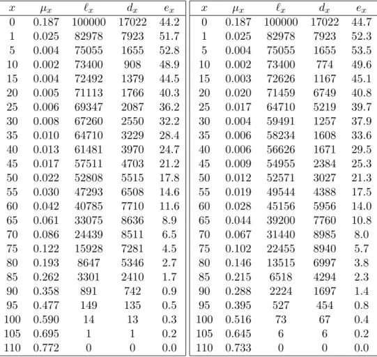
You may have noticed a logical fallacy in the arguments of sections 3.4 and 3.5. The life expectancy at birth should be the average length of life of individuals born in that year. Of course, we would have to go back to about 1890 to find a birth year whose cohort — the individuals born in that year — have completed their lives, so that the average lifespan can be computed as an average.
Consider, for instance, the discrete-time non-homogeneous model. “Time” in the model is individual age: An individual starts out at age 0, then progresses to age 1 if she survives, and so on. We estimate the probability of dying aged xby dividing the number of deaths observed agex by the number of individuals observed to have been at that age.
In our life-tables, called period life tables, these numbers came from a census of the in-dividuals alive at one particular time, and the count of those who died in the same year, or period of a few years. No individual experiences those mortality rates. Those born in 2009 will experience the mortality rates for age 10 in 2019, and the mortality rates for age 80 in 2089. Putting together those mortality rates would give us acohort life table. (Actually, this is not precisely true. You might think about why not. The answer is given in a footnote.1) If, as has been the case for the past 150 years, mortality rates decline in the interval, that means that the survival rates will be higher than we see in the period table.
We show in Figure 4.1 a picture of how a cohort life table for the 1890 cohort would be related to the sequence of period life tables from the 1890s through the 2000s. The mortality rates for ages 0 through 9 (thus 1q0, 4q1, 5q5)2 are on the 1890s period life table, while their
mortality rates for ages 10 through 19 are on the 1900–1909 period life table, and so on. Note that the mortality rates for the 1890s period life table yield a life expectancy at birthe0 = 44.2
years. That is the average length of life that babies born in those years would have had, if their mortality in each year of their lives had corresponded to the mortality rates which were realised in for the whole population in the year of their birth. Instead, though, those that survived their
1
The main difference between a cohort life table and the life table constructed from the corresponding age classes of successive period life tables is immigration: The cohort life table for 1890 should include, in the row for (let us say) ages 60–4 the mortality rates of those born in 1890 in the relevant region — England and Wales in this case — who are still alive at age 60. But these are not identical to the 60 year old men living in England and Wales in 1950. Some of the original cohort have moved away, and some residing in the country were not born there.
2
Actually, we have givenµx for the intervals [0,1), [1,5), and [5,10). We compute1q0 = 1−e−µ0, 4q1 =
1−e−4µ1,
5q5= 1−e−5µ5.
early years entered the period of late-life high mortality in the mid- to late 20th century, when mortality rates were much lower. It may seem surprising, then, that the life expectancy for the cohort life table only goes up to 44.7 years. Is it true that this cohort only gained 6 months of life on average, from all the medical and economic progress that took place during their lives?
Yes and no. If we look more carefully at the period and cohort life tables in Table4.1we see an interesting story. First of all, a substantial fraction of potential lifespan


![Table 3.1: Male mortality data for England and Wales, 1990–2. From [Fox97] (available online at http://www.statistics.gov.uk/StatBase/Product.asp?vlnk=333).](https://thumb-us.123doks.com/thumbv2/123dok_us/694220.2585357/33.918.205.699.145.1038/table-mortality-england-wales-available-statistics-statbase-product.webp)