Thermo-Calc Console Mode
User Guide
Version 3.1
© 1995-2013 Foundation of Computational Thermodynamics
Stockholm, Sweden
1
Thermo-Calc Console Mode
User Guide
Contents
1 Introduction ... 3
1.1 The Thermo-Calc software package ... 3
1.2 Documentation for Thermo-Calc Console Mode ... 3
1.2.1 This User Guide ... 4
1.2.2 Using online help ... 4
1.2.3 Contents of the Thermo-Calc Console Examples Collection ... 5
1.3 Program overview ... 5
1.3.1 Modules ... 5
2 Using the console interface... 7
2.1 The Thermo-Calc Console Mode interface ... 7
2.2 Using the command line prompt ... 9
2.2.1 Command names and abbreviations ... 9
2.2.2 Specifying parameters ... 10
2.2.3 Default parameters values ... 10
2.2.4 Controlling Console output ... 11
2.2.5 Command history ... 11
2.2.6 Wild card characters ... 12
2.3 Using log, macro, and workspace files ... 13
2.3.1 Using log files ... 13
2.3.2 Using macro files... 13
2.3.3 Using workspace files ... 15
2.4 Default options ... 15
2.5 Workflow ... 16
2.5.1 Moving between modules and submodules ... 17
2.5.2 Typical workflow when using POLY ... 17
3 Defining a system ... 19
3.1.1 How to define your system ... 19
4 Calculation ... 21
4.1 Equilibrium ... 21
4.1.1 How to calculate an equilibrium ... 23
4.1.2 Variations ... 24
4.2 Property diagrams ... 24
2
4.2.2 Variations ... 26
4.3 Phase diagrams ... 27
4.3.1 How to calculate and plot a phase diagram ... 28
4.3.2 Variations ... 29
4.4 Scheil simulations ... 30
4.4.1 How to simulate a Scheil-solidification ... 31
4.4.2 How to plot additional Scheil simulation diagrams ... 34
4.4.3 How to run additional simulations on your alloy system ... 35
4.5 T0 temperature simulations ... 36
4.5.1 How to make a T0 temperature simulation ... 36
4.6 Paraequilibrium ... 38
4.6.1 How to calculate a paraequilibrium ... 38
4.7 Potential diagrams ... 40
4.7.1 How to calculate a potential diagram in POTENTIAL .. 40
4.7.2 How to calculate a potential diagram with different pressure ... 42
4.8 Aqueous solutions ... 43
4.8.1 How to calculate a Pourbaix diagram ... 44
4.8.2 How to plot additional aqueous solution diagrams ... 46
4.8.3 How to do a stepping calculation on an aqueous solution ... 47
4.9 Tabulation of chemical substances, phases or reactions ... 48
4.9.1 How to tabulate a reaction ... 49
4.9.2 How to tabulate a substance or solution phase at fixed composition ... 50
5 Visualization ... 51
5.1.1 How to plot your diagram ... 52
5.1.2 Modifying your diagram ... 53
5.1.3 Saving your diagram ... 54
5.1.4 Loading a previously saved diagram ... 55
6 Appendix 1 – List of examples in the Thermo-Calc Console Examples Collection ... 56
3
1
Introduction
1.1
The Thermo-Calc software package
Thermo-Calc is a sophisticated software, database and programming-interface package for performing thermodynamic calculations. It allows you to calculate complex homogeneous and heterogeneous phase
equilibria, and plot the results as property diagrams and phase diagrams. The program fully supports stoichiometric and non-ideal solution models and databases. These models and databases can be used to make
calculations on a large variety of materials such as steels, alloys, slags, salts, ceramics, solders, polymers, subcritical aqueous solutions, supercritical electrolyte solutions, non-ideal gases and hydrothermal fluids or organic substances. The calculations can take into account wide ranges of
temperature, pressure and compositions conditions.
A Software Development Kit (SDK) is available for the Thermo-Calc
program. This SDK can be used to plug the Thermo-Calc calculation engine into your own applications or into various third-party applications. There are two interfaces to the Thermo-Calc program, the Console Mode which uses a command line interface and the Graphical Mode which has a graphical user interface (GUI). This User Guide describes the use of the Thermo-Calc program in the Console Mode.
1.2
Documentation for Thermo-Calc Console Mode
Apart from this document, you can use the following documentation to learn more about how to use Thermo-Calc in the Console Mode: Thermo-Calc Console Mode Command Reference
contains information about all the commands that are available in the Thermo-Calc Console. For each command there is a brief description of what the command does, what the command’s parameters are (if any), and what kind of values you can give the parameters
Online help in the Thermo-Calc Console Mode
contains information about modules, commands, and conditions
Thermo-Calc Console Examples Collection
contains over fifty example macro files that demonstrate different ways in which you can use Thermo-Calc. See Appendix 1 – List of examples in the Thermo-Calc Console Examples Collection DATAPLOT User’s Guide and Examples
describes the syntax and semantics of the DATAPLOT graphical language, which is used to store information about thermodynamic diagrams Additional documentation and educational materials are available on Thermo-Calc Software’s website.
4
1.2.1
This User Guide
Target group
This user guide is intended for new users of the Thermo-Calc console mode that are not familiar with the command-line interface. It is expected, however, that such a user does understand the basics of thermodynamics.
Purpose
This Thermo-Calc Console Mode User Guide is intended to get you started using Thermo-Calc in the Console Mode. It gives you a brief overview of the program and its various components, describes how the command line user interface works, and describes how, in generic terms, you can define your system of components, set up calculations, perform calculations and visualize the results.
Content
After this Introduction chapter, chapters 2 to 4 describe steps in the typical Thermo-Calc workflow. Chapter 2 describes how you define which
elements your system contains and retrieve necessary thermodynamic data about these elements. Chapter 3 describes how you set up and perform various kinds of calculations, and plot the results as property or phase diagrams of various kinds. Finally, chapter 4 describes how you can modify how a diagram is plotted, change the appearance of your diagram, and save it in different formats.
Note that this User Guide only scratches the surface of what you can do with Thermo-Calc. Thermo-Calc is a very powerful and flexible program. At every stage in the workflow, there are a host of different parameters and conditions that you can modify to tweak and tune your material system, the calculation, or the visualization of the results. Once you have learned the basics from this User Guide, you can turn to other learning resources. Thermo-Calc can be used in two interface modes: the Console Mode and the Graphical Mode. This guide only describes how you use Thermo-Calc in the Console Mode. For information about how to use Thermo-Calc in the Graphical Mode, see the Thermo-Calc Graphical Mode User Guide.
The following conventions will be used:
Console command name are written in small upper case letters. For example, the command for calculating an equilibrium is
COMPUTE_EQUILIBRIUM.
Examples of how you can use a command are written like this: SET_CONDITION T=1000 P=1E5 X(C)=0.01 N=1
Menu items are referred to by the menu name and the name of the item, separated by a vertical line (“|”). For example, “select Tools | Options” means, select the menu item “Options” from the Tools main menu.
1.2.2
Using online help
At the command line prompt in the Console, you can access online help information in several ways:
5
To get a list of all the available commands in the current module, simply type a question mark (“?”) and press the enter key.
To get a description of a specific command, use HELP followed by the
name of the command. Note that you can only get online help information about a command that is available in the module that you are currently in.
To get more general information about the system, use INFORMATION.
You will be requested to specify about which subject you want information. Answer “?” in response and you will get a list of all the subjects on which you can get more information. Note that this subject list is specific to the module you are currently in.
To access some online help that you can read in a web browser, select “Help | Help Contents”. From this help contents, it is also possible to access some documentation available as PDF-files, including this User Guide.
1.2.3
Contents of the Thermo-Calc Console Examples Collection
To learn more about how to use Thermo-Calc, you can run and study the examples in the Thermo-Calc Console Examples Collection. This is a
collection of extensively commented macro files that you can either run in Thermo-Calc, or open and read in a text editor. If you read the macro file in a text editor, you will not see the output that Thermo-Calc gives in
response to the commands stored in the macro file. However, the pdf document Thermo-Calc Examples also shows the output for each example. A table provides a brief description of each example in Appendix 1 – List of examples in the Thermo-Calc Console Examples Collection.
1.3
Program overview
The Thermo-Calc program consists of several basic modules that handle database retrieval and management, calculation and optimization, and visualization and diagram plotting.
Most modules are managed using commands but some modules, called response-driven modules, prompt you with a series of questions which typically take you through the whole process of defining your system, setting conditions on the calculation, performing the calculation and plotting the results.
1.3.1
Modules
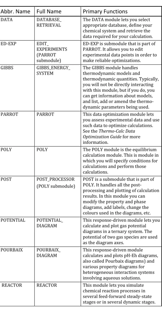
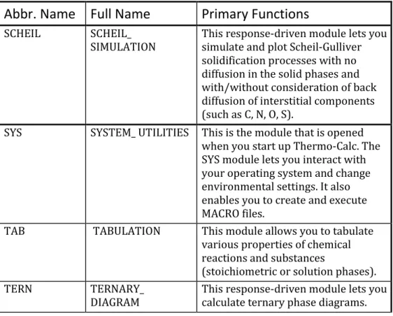
The following table lists and briefly describes Thermo-Calc’s various modules:
Abbr. Name Full Name
Primary Functions
BIN BINARY_ DIAGRAM This response-driven module lets you calculate binary phase diagrams. To use this module, you need access to databases that were designed for the BIN module, such as the TCBIN database.
6
Abbr. Name Full Name
Primary Functions
DATA DATABASE_
RETRIEVAL The DATA module lets you select appropriate database, define your chemical system and retrieve the data required for your calculation. ED-EXP EDIT_
EXPERIMENTS (PARROT submodule)
ED-EXP is submodule that is part of PARROT. It allows you to edit experimental data points in order to make reliable optimizations.
GIBBS GIBBS_ENERGY_ SYSTEM
The GIBBS module handles thermodynamic models and
thermodynamic quantities. Typically, you will not be directly interacting with this module, but if you do, you can get information about models, and list, add or amend the thermo-dynamic parameters being used. PARROT PARROT This data optimization module lets
you assess experimental data and use such data to optimize calculations. See the Thermo-Calc Data
Optimization Guide for more information.
POLY POLY The POLY module is the equilibrium calculation module. This is module in which you will specify conditions for calculations and perform those calculations.
POST POST_PROCESSOR
(POLY submodule)
POST is a submodule that is part of POLY. It handles all the
post-processing and plotting of calculation results. In this module you can modify the property and phase diagrams, add labels, change the colours used in the diagrams, etc. POTENTIAL POTENTIAL_
DIAGRAM This response-driven module lets you calculate and plot gas potential diagrams in a ternary system. The potential of two gas species are used as the diagram axes.
POURBAIX POURBAIX_ DIAGRAM
This response-driven module
calculates and plots pH-Eh diagrams, also called Pourbaix diagrams) and various property diagrams for heterogeneous interaction systems involving aqueous solutions. REACTOR REACTOR This module lets you simulate
chemical reaction processes in several feed-forward steady-state stages or in several dynamic stages.
7
Abbr. Name Full Name
Primary Functions
SCHEIL SCHEIL_
SIMULATION This response-driven module lets you simulate and plot Scheil-Gulliver solidification processes with no diffusion in the solid phases and with/without consideration of back diffusion of interstitial components (such as C, N, O, S).
SYS SYSTEM_ UTILITIES This is the module that is opened when you start up Thermo-Calc. The SYS module lets you interact with your operating system and change environmental settings. It also enables you to create and execute MACRO files.
TAB TABULATION This module allows you to tabulate various properties of chemical reactions and substances
(stoichiometric or solution phases).
TERN TERNARY_
DIAGRAM This response-driven module lets you calculate ternary phase diagrams.
2
Using the console interface
This section briefly introduces you to the Console Mode’s user interface and the command line prompt. You can also read about how to save your work in Thermo-Calc. The basic workflow of the program is also described.
2.1
The Thermo-Calc Console Mode interface
When you open Thermo-Calc, the program will by default be opened in the Graphical Mode. To enter Console Mode, click »Switch to Console Mode» on the toolbar.
The following screen shot shows the Thermo-Calc Console Mode user interface:
8
There are three types of windows:
“Console” Is placed by default on the left side of the screen. This is where you type your commands. You can open additional Console windows by pressing “Ctrl-T” or by clicking the »Add button» “Console Results”
Is placed by default on the right side of the screen. This is where diagrams that are plotted will
appear. Each Console has its own Results tab in the Console Results window. All the plots and tables generated from the console will be presented in that Results tab. You can open new additional Plot tabs by pressing “Ctrl-Shift-T” or by clicking the »Add button»
.
“Event Log” This window is opened by you and displays information about the commands that run and are completed, including any error messages..
If you close any of these windows, you can open them again by selecting the “Console”, “Console Results” or “Event Log” item on the “Windows” menu. To realign the windows to the original layout, select Windows | Reset Windows.
By default, different tabs are presented as one on top of each other in the following way:
9
To view as certain tab, simply click on the header of that tab. You can also view tabs laid out side-by-side or top-to-bottom in both the Console and the Console Results window. Do this by clicking the «Show tabs side by side button» or the «Show tabs stacked button» . To return to showing the tabs on top of each other as in the preceding screen shot, click the «Tab label button» .
2.2
Using the command line prompt
The command line prompt in the Console window tells you which module you are currently in. When you open Thermo-Calc in the Console Mode, you will find yourself in the SYS module, and this is indicated by the fact that the command line prompt is “SYS:”
To use Thermo-Calc in the Console Mode, you type in commands at the command line prompt. Which commands are available to you depends on which module you are in. To see a list of all the commands that are available in the module you are in, type “?” and press the enter-key.
2.2.1
Command names and abbreviations
The name of a command typically consists of several terms linked by underscore characters, such as LIST_EQUILIBRIUM. It does not matter
whether you type in commands in upper or lower case letters.
You can abbreviate all Thermo-Calc commands as long as the abbreviation is unambiguous. Each word in the command name can be abbreviated separately. For example, LIST_EQUILIBRIUM can be abbreviated L_E. Instead of
the underscore character, you can separate the words in a command name by a hyphen (“-”).
The following table shows examples of how you can abbreviate some command names:
Command name
Abbreviation
CALCULATE_EQUILIBRIUM C-E CALCULATE_ALL_EQUILIBRIA C-A LIST_EQUILIBRIUM L-E LIST_INITIAL_EQUILBRIUM LI-I-E LOAD_INITIAL_EQUILBRIUM LO-I-E LIST_PHASE_DATA CBCC L-P-D CBC LIST_PHASE_DATA CEMENTITE L-P-D CEM SET_ALL_START_VALUES S-A-S
S-AL
SET_AXIS_VARIABLE 1 X(FCC,FE)00.890.025 S-A-V 1 X(F,FE)0.89.025 SET_START_CONSTITUENT S-S-C
SET_START_VALUE S-S-V SET_AXIS_PLOT_STATUS S-A-P SET_AXIS_TEXT_STATUS S-A-T-S
10
SET_AXIS_TYPE S-A-TY SET_OPTIMIZING_CONDITION S-O-C SET_OPTIMIZING_VARIABLE S-O-V SET_OUTPUT_LEVEL S-O-L S-OU
2.2.2
Specifying parameters
Running a command typically requires that a number of parameter values be specified. Parameters can be specified directly at the command line after the command name. For example, to set an axis variable for a stepping or mapping operation, you could directly enter:
SET_AXIS_VARIABLE 1 X(FCC,FE) 0 0.89 0.025 Alternatively, you could type SET_AXIS_VARIABLE and simply press the enter
key. At the command line prompt, you would then be requested to specify the parameters one by one.
If you are not sure what your alternatives are, or what the requested parameter is, then you can try answering with a question mark (“?”). Typically, a brief explanation will then follow. For some parameters, more detailed information will be presented if you answer with two question marks (“??”).
2.2.3
Default parameters values
When you are requested to specify a parameter, Thermo-Calc usually suggests an appropriate default value or answer. Such a default value or answer is given between two slash signs (“/”) at the prompt. For example, the following prompt indicates that the default answer is “terminal”:
OUTPUT FILE /TERMINAL/:
To accept the default value or answer, simply press the enter key.
If you specify some parameters directly after the command name, then you can still choose to accept default values for some parameters. To accept the default value for a parameter, type a comma (“,”) instead of a value for that parameter. For the comma to be interpreted correctly, type a blank space on each side of the comma. However, if you accept the default values for several parameters that follow each other, then the commas can be typed in without blank spaces separating them (“ ,,, ” will be interpreted in the same way as “ , , , ”).
For some commands and parameters, Thermo-Calc treats the values that you have previously assigned to them as default values if the command is used again. For example, suppose that the first stepping or mapping axis variable is specified in the following way:
SET_AXIS_VARIABLE 1 X(FCC,FE) 0 0.89 0.025 If you later want to change one parameter value for this axis variable, then you could type:
11
This will change the minimum value from 0 to 0.1 at which a stepping or mapping operation will halt. The other parameter values will remain the same. Consequently, what you typed in would be equivalent to the following:
SET_AXIS_VARIABLE 1 X(FCC,FE) 0.1 0.89 0.025
2.2.4
Controlling Console output
Thermo-Calc may print a lot of text in the Console window in response to a command. You can pause the printing of the output by pressing “Ctrl-S”. To resume the printing on screen, press “Ctrl-Q”.
Occasionally, the output to screen can overflow the text buffer of the window. If this happens, then it may be useful to increase the buffer size of the current Console tab.
How to increase the buffer size
To increase the buffer size in a certain Console tab, perform the following two steps:
Step
Action
1 Right-click on the Console tab header in the Console window (if this is the first Console tab, it will be labelled “Console 1”) 2 Click on “Properties”, and then increase the “Buffer size” in the
Console Properties window.
Note that this only changes the buffer size of the particular tab whose header you right-clicked. To change the buffer size of any new tabs that you will create, select Tools | Options, then select the “Console Mode” tab where you can increase the default “Buffer size”.
When Thermo-Calc is performing a mapping operation, the results will be continuously printed in the Console window. To terminate the calculation of the current region of the mapping and stop the output, press “Ctrl-C”.
2.2.5
Command history
To scroll through the last twenty commands that you have used, type two exclamation marks (“!!”) and press the enter key. To repeat the last n commands, type “!” followed by the number of previous commands that should be executed again. To scroll through previous performed
commands, use the Up or Down arrow keys (“” or “”).
To read more information about the command history functionality in Thermo-Calc, type “! ?” at the command line prompt.
12
2.2.6
Wild card characters
You can sometimes use the asterisk (“*”) as a wild card character to, for example, refer to all components, all phases, or all species. For instance, you can do this when showing calculated properties in the POLY module, or when you set axis variables for plotting diagrams in the POST module. When showing calculated properties in the POLY module, you can also use the dollar sign (“$”) to refer to all stable phases. The asterix and the dollar sign normally does not work properly as wild card characters for referring to activity and/or chemical potential properties.
The following table shows ways in which you can use these wild card characters.
Command
Action
SHOW_VALUE B(*) Lists mass (gram) of all components
in the system.
SET_AXIS_VAR Y B(*)* Sets mass (gram) of all components in
the system as Y-axis variable.
SHOW_VALUE MUR(*) Lists chemical potentials of all
components in the system.
SET_AXIS_VAR Y ACR(*)* Sets activities of all components in the
system as Y-axis variable.
SHOW_VALUE HM(*).T Lists heat capacities of all phases. SET_AXIS_VAR Y GM(*)* Sets molar Gibbs free energies of all
phases as Y-axis variable.
SHOW_VALUE TC($) Lists curie temperature of all stable
phases.
SHOW_VALUE W(*,*) Lists mass fractions of all components
in all phases.
SHOW_VALUE W($,*) Lists mass fractions of all components
in all stable phases.
SHOW_VALUE W(FCC,*) Lists mass fractions of all components in the FCC phase.
SHOW_VALUE W(*,FE) Lists mass fractions of the Fe
component in all phases.
SHOW_VALUE W($,FE) Lists mass fractions of the Fe
component in all stable phases.
SHOW_VALUE Y(*,*) Lists site fractions of all species in all
sublattices of all phases.
SHOW_VALUE Y($,*) Lists site fractions of all species in all
sublattices of all stable phases.
SHOW_VALUE Y(*,*) Lists site fractions of all species in all
13
2.3
Using log, macro, and workspace files
In the console mode, Thermo-Calc makes use of a few different kinds of files, including log files (*.LOG), macro files (*.TCM or *.LOG), POLY workspace files (*.POLY3), and experimental data files (*.EXP). The GIBBS module makes use of its own type of workspace files (*.GES5), and the PARROT module makes use of files with the suffixes *.PAR and *.POP. When you start using Thermo-Calc in the console mode you will mainly make use of log files, macro files and POLY workspace files.
For information about experimental data files, see the DATAPLOT User Guide and the Thermo-Calc Data Optimization Guide.
2.3.1
Using log files
Log files are are plain text files used to save a sequence of commands. Log files can be edited in a text editor.
To start saving your input into such a file, use SET_LOG_FILE in the SYS
module, followed by the name of the file that you want to save your command sequence to.
If you want to save Thermo-Calc’s output in the log file as well, use
SET_ECHO before the SET_LOG_FILE command. Doing this is often useful if you
want use the log file later as a macro file.
2.3.2
Using macro files
Macro files are plain text files used to save a sequence of commands that can be loaded and executed. Macro files can be edited in a text editor. To load a macro file, use MACRO_FILE_OPEN in the SYS module, followed by the
name of the macro file. Thermo-Calc will then immediately execute the command sequence that the file contains.
If you end a macro file with the SET_INTERACTIVE command, then control of the Console will be given back to the user.
You can make a macro file load other macro files inside it by adding a
MACRO_FILE_OPEN command when creating the log file that you want to use as a macro file. You can in this way have at most five nested levels of macro file. If a nested macro file ends with SET_INTERACTIVE, then Thermo-Calc will
resume with the higher-level macro file at the command immediately following after the MACRO_FILE_OPEN command that loaded and executed
macro file that has just been terminated. If a nested macro file doesn’t end with SET_INTERACTIVE (but with an end-of-file character), then the console
will shut down and the macro will be aborted.
You add comments to a macro file by starting a line with “@@”, or by enclosing them between a “@(“-line and a “@)”-line. All lines in the macro file that are between these lines will be ignored by Thermo-Calc when you are running the macro.
14
Control characters
The “@?” character allows you to make a macro interactive by allowing input from the user. At the “@?” character, which should be placed where a parameter value or argument would normally be put, Thermo-Calc will prompt the user to input the value of a parameter or argument. You can enter a string immediately following the “@?”-character. This string will be presented to the user when prompted to enter the parameter value or argument. The entered value will be used by Thermo-Calc as input to the command in question. For example, you can request the user to specify the temperature range of a stepping calculation by entering the following in a macro file:
SET_AXIS_VARIABLE 1 T @?Low-temperature-limit: @?High-temperature-limit:
You can also use up to nine variables in your macro file and prompt the user to enter values that can be assigned to these variables. Use the “@#n” character when you want to prompt the user to provide a value to the variable, where the ‘n’ is digit between ‘1’ and ‘9’. You can then use this value by with the “##n” character. For example, you can request the user to provide the first element of a system by entering the following in the macro file:
@#3First-element?
You can then use this variable with the entering the character “##3” later in the macro file. For example, you could write:
SET_AXIS_VARIABLE 1 x(##3) 0 1,,,
Finally, there is the “@&” pause character. Thermo-Calc pauses and waits for input from the user when this pause character is read from a macro file. Inserting pause characters is useful if you want to allow the user to
monitor what is happening when Thermo-Calc is running the macro.
Response-driven modules and macros
Macro files that are created while you use a response-driven module begin with the module-entering command (for example, GOTO_MODULE SCHEIL)
followed by a number of lines with responses to the module’s questions and requests. The file terminates with the POST or the SET_INTERACTIVE
command (this command gives you back control of the Console). An empty line cannot be edited with any input rather than the default answer (to a specific question). Comment lines, commands to open other macro files, pause characters or input-controlling characters cannot be inserted between these empty lines (otherwise the response-driven module cannot be executed properly).
15
2.3.3
Using workspace files
You can save all the data in your current workspace by first using
SAVE_WORKSPACES. This command is available in the POLY module, as well as
in the GIBBS and PARROT modules. The workspace will contains all the settings you have specified and the result of any stepping or mapping operations that you have performed after using SAVE_WORKSPACES.
Consequently, the command opens a workspace in which all data is saved which is generated after the SAVE_WORKSPACE command has been executed.
The saved data will include original and modified thermodynamic data, your last set of conditions and options, and the results of any calculations. To load the data and calculation results of a workspace file, use the
READ_WORKSPACES command that is available in the POLY module. The file
can be used for calculation in POLY, visualization in POST, or data
manipulation in GIBBS. You are also given the option in the POURBAIX and SCHEIL modules to open a previously saved workspace file. This allows you to make new POURBAIX or SCHEIL calculations on the same chemical system as before but with different temperature, pressure, and
composition conditions, or to plot new property diagrams based on the previous calculations.
When you go to a response-driven module such as POTENTIAL or SCHEIL for example, a workspace file will automatically be opened. In the
workspace file, system definitions, conditions for the calculation,
calculation results, and plot settings will be saved. The file will be saved in the current working directory, and will be named after the name of the module that created it. For example, the POTENTIAL module will save a workspace file called POT.POLY3 (or POT.poly3 in Linux); the POURBAIX module will save a file called POURBAIX.POLY3; etc.
2.4
Default options
You can set general settings for Thermo-Calc Console mode in the
“Options” window. To open this window, select “Options” from the “Tools” main menu. The tabs and panes that are relevant for Thermo-Calc Console mode are briefly described in the table that follows:
Tab / pane
Description
General Here you can select whether to turn
on tooltips information. If “Tooltips enabled” is selected, then a small text box will appear when you hold the cursor still above some buttons or other items.
Here you can also select which language that will be used in the program, and change the
appearance of the program (“Look and feel”).
In the “Database directory” field, specify in which directory the Thermo-Calc database directory called “data” can be found. Note that
16
you are not supposed to specify the path to where the database files can be found (that is, in the “data” directory), but the path to the directory that contains the “data” directory.
Adjust the “Log Level” slide bar to get more or less information presented in the “Event Log” window.
Default appearance Here you can specify the default name, buffer size, fonts and colours that are used for new Console windows. You can also set the default directory where log files and workspace files are saved.
To change the name, buffer size, fonts and colours for a specific Console window, right-click on the label for that particular Console and select “Properties” from the pop-up menu.
Console Mode>Plotting Here you can change the default settings for any diagrams that will be plotted. Note that these settings are shared with the Thermo-Calc Graphical mode. Any changes you make here will also apply to the default settings on the Graphical Mode>Activities>Plotting tab in the “Options” window (and vice versa). You can also change the settings for plotting locally for a certain plot in the Console Results window, by right-clicking on the plot and selecting “Properties” from the pop-up menu.
In addition, the colour, stroke (solid/dashed/dotted/dash_dot) and line width of a particular series of lines in a plot can be changed by double-clicking on one of the lines in that series.
2.5
Workflow
Working with Thermo-Calc involves moving between different modules. The workflow will differ depending on the kind of calculation you want to perform:
17
If you want to perform a calculation using the POLY module, you typically first retrieve thermodynamic data in the DATA module, perform the calculation in POLY, and visualize the results in the POST module. This workflow is described below. (However, it is possible to define a system directly in POLY using DEFINE_MATERIAL and
DEFINE_DIAGRAM).
If you want to calculate and plot a diagram using a response-driven module, such as POTENTIAL or SCHEIL, then you can go directly to that module. Response-driven modules will prompt you to go through each step necessary for performing the calculation and the required post-processing. These modules include BIN, TERN, POTENTIAL, POURBAIX, and SCHEIL. You typically end up in the POST module after having used a response-driven module. In the POST module you can modify the plotting in various ways and save the diagram in various formats.
If you want to tabulate a chemical substance, phase, or reaction, go directly to the TAB module. For more information, see section 4.9.
2.5.1
Moving between modules and submodules
To go to a specific module, you typically use GOTO_MODULE followed by the
name of the module. For example, if you want to go to the DATA module, type the following:
GOTO_MODULE DATA
The exceptions are the submodules POST and ED-EXP. To go to the POST module, you must use POST, a command that is only available in the POLY
module. To go to the ED-EXP module, you must use ED-EXP, a command that
is only available in the PARROT module.
To go back to the module you came from when entering the module you are currently in, use BACK. For example, if you entered the DATA module
from the SYS module and use BACK, you will go back to the SYS module.
Note that you must use BACK to leave the submodules POST and ED-EXP.
The GOTO_MODULE command is not available in these submodules.
2.5.2
Typical workflow when using POLY
The following figure represent the typical workflow when you perform calculations in the POLY module. The solid arrows represent your typical movements between the modules. The dashed arrows represent movement of data within Thermo-Calc.
18
The basic workflow is the following:
1 When you start Thermo-Calc in the Console Mode, you find yourself in the SYS module.
2 Define your system in the DATA module: Before performing your calculation, you must define your system and retrieve
thermodynamic data. See chapter 3 for more information. The data is retrieved from a database file (*.TDB or *.TDC), and the data needed for describing your system is sent to the GIBBS module. This data is then accessed by the POLY module when you instruct it to perform calculations.
3 Perform the calculation in the POLY module: In POLY, you first set the conditions for an equilibrium calculation (temperature, pressure, system composition, etc.), then do the equilibrium calculation. If you want to go on and make a property or phase diagram, you set the conditions for a stepping or mapping
operation and perform that operation. This will generate data that can be used to plot a property diagram (if you performed a
stepping operation) or a phase diagram (if you performed a mapping operation). See chapter 4 for more information.
19
4 Plot and visualize your data in the POST module: If you have performed a stepping or mapping operation, then you can go to the POST module and plot a property of phase diagram. The diagram can be plotted quickly using default settings, but you can also modify which variables to plot of the diagram axes and change the appearance of the diagram in a host of ways. You can save the diagram either as a plain text file with data about all the coordinates or as an image file (in many different formats). See chapter 5 for more information.
3
Defining a system
Selecting the chemical components on which a calculation is to be run is called defining a system. To do this, you need to make use of some database(s) with thermodynamic, and then define which elements that your system will have as components. Once you have defined your system, you have to retrieve thermodynamic data for the system from the
database(s).
If you use a response-driven module to perform your calculation, such as BIN or POURBAIX for example, then that module will prompt you to select database(s) and define your system. When performing calculations in the POLY module, you will typically have to manually select databases and define your system in the DATA module. This section describes how to do this. However, note that it is also possible to define the system directly in POLY using DEFINE_MATERIAL and DEFINE_DIAGRAM (see the Thermo-Calc Console Mode Command Reference for information about these commands).
3.1.1
How to define your system
To define your system means to select its components and to retrieve thermodynamic data about those components from an appropriate database. This section describes how you do this in the DATA module.
Pre-requisites
To define your system, you must be in the DATA module. Use GOTO_MODULE DATA to enter it.
Procedure
To define your system, follow these steps:
Step
Action
5 Use SWITCH_DATABASE to change your default database. Unless you
directly specify the name of the database as a parameter to the command, then the available databases will be listed, and you will be prompted to specify which you want to use.
The second part of the command prompt indicates the current default database. For example, if the prompt reads “TDB_TCFE7:”, then this means that the current database is TCFE7.
20
6 Use DEFINE_ELEMENTS followed by a list of the elements that you
want in your system. (To list the elements that are available in your current database, use LIST_DATABASE ELEMENTS.) For example,
if you want to have Fe and C in your system, you would type: DEFINE_ELEMENTS Fe C
7 Use REJECT PHASES if you want to avoid retrieving any phases from
the database. (To list the phases that are available in your current database, use LIST_DATABASE PHASES. To list the phases that can
form in the defined system, use LIST_SYSTEM CONSTITUENT.) For
example, if you do not want the graphite phase to be retrieved, you would write:
REJECT PHASES GRAPHITE
If the number of phases that should be included is much lower than the total number of phases, then it may be convenient to first reject all phases using REJECT PHASES * and then restore the phases
that should be included using RESTORE PHASES.
8 Use GET_DATA to search the database and send the thermodynamic data about your system to the GIBBS workspace.
At this point you can proceed to the POLY module (with
GOTO_MODULE POLY). However, you may want to add elements, phases and species to the GIBBS workspace from other databases. If so, then proceed to the next step.
9 Use APPEND_DATABASE to select the (additional) database from
which you want to retrieve data. This command works exactly in the same way as the SWITCH_DATABASE command, with the
exception that it does not reinitialize the DATA module and the GIBBS workspace, but instead appends or replaces the data that has already been retrieved with new data from the additional database.
10 Define your elements and specify whether to reject and restore any phases. Do this in exactly the same way as you would using the SWITCH_DATABASE command (see the preceding steps 2 and 3).
11 Use GET_DATA to search the database and add the thermodynamic
data to the data that already exists in the GIBBS workspace. Use APPEND_DATABASE again if you want to add data from yet
another database. When you have retrieved all the data you need, you can proceed to the POLY module.
21
4
Calculation
This chapter describes some of the most common calculations performed in Thermo-Calc. Calculations can be performed either in the POLY module, or using some of the response-driven modules that have been designed to enable you do perform some specific type of calculation.
The first three sections of this chapter describes, in very general terms, how to perform an equilibrium calculation, calculate and plot a property diagram, and calculate and plot a phase diagram. There is an endless variety of calculation types that can be plotted as property or phase diagrams. What follows are descriptions of a basic kind of calculation. At each section, a few ways in which you can change settings or conditions are also described.
Note that to calculate and plot a property diagram or a phase diagram, you must first calculate an equilibrium. The first section therefore describes how to calculate a single-point equilibrium.
4.1
Equilibrium
An equilibrium describes what the composition of the end state of your system will be, given a full specification of state variables such as
temperature, pressure, initial composition, system size, etc. An equilibrium calculation is normally performed in POLY according to the Global
Minimization Technique, which assures that the most stable minimum under the specified conditions is computed.
For an equilibrium calculation to be performed, the state variables must all be set as conditions for the calculations. Such conditions include, for example, temperature, pressure, and system composition. When you calculate an equilibrium in the POLY module, you have to set these conditions manually.
Setting a condition normally involves giving a single state variable a specific value. For example, you can set the temperature to 1273.5 Kelvin (“T=1273.5”). Alternatively, setting a condition can involve giving a linear expression with more than one state variable a specific value. For example, you can set the mole fraction of the S component to be the same in the liquid and the pyrrohotite phases (“X(LIQ,S)-X(PYRR,S)=0”).
The number of state variables that needs to set is determined by the Gibbs Phase Rule (see Educational Material). Typically, the state variables that you need to give values to are the following:
temperature (in K)
pressure (in Pascal)
system size in number of moles (in mole) or mass (in grams)
22
The following table lists some of the state variables that are available and that you can use to set conditions:
State variable
SET_CONDITION parameter
temperature in the system (in K) T pressure in the system (in Pascal) P system size (mole number in moles) N system size (mass in grams) B number of moles of a component in the
system N(<component>)
mole fraction of a component in the
system X(<component>)
mass fraction of a component in the
system W(<component>)
activity of a component in the system ACR(<component>) chemical potential of a component in
the system MUR(<component>)
mole fraction of a component in a
phase X(<phase>,<component>)
mass fraction of a component in a
phase W(<phase>,<component>)
activity of a species referred to a phase
at ambient temperature and pressure ACR(<species>,<phase>) chemical potential of a species referred
to a phase at ambient temperature and pressure
MUR(<species>,<phase>)
enthalpy in the system (in J) H
enthalpy of a phase (in J/mol) HM(<phase>)
If you fix the phase of the equilibrium and all but one of the state variables, you can discover the value of the other state variable at equilibrium. It is possible to specify a set of conditions that does not have any equilibrium and the program will detect this simply by failing to reach equilibrium during the calculation.
Here is an example of the kind of information about the equilibrium that will normally be presented to you:
23
4.1.1
How to calculate an equilibrium
This section explains how to calculate an equilibrium in POLY. To calculate an equilibrium means to calculate the equilibrium composition of your system, given a full specification of conditions that reduce the degrees of freedom of the calculation to zero.
Pre-requisites
Before calculating an equilibrium, you must have defined your system and entered POLY.
Procedure
To calculate an equilibrium, follow these steps:
Step
Action
1 Use SET_CONDITION followed by conditions and value assignments
to set the conditions of your calculation. For example, to set temperature, pressure, initial composition and system size for a Fe-Cr-C system, you might enter the following:
SET_CONDITION T=1200 P=1E5 W(CR)=0.18 W(C)=0.0013 N=1
This sets the temperature (T) to 1200 K, the pressure to 1 bar (100,000 Pascal), the mass fraction of Cr to 18 mole percent, the mass fraction of C to 0.13 weight percent, and the total amount of material to 1 mole. The fraction of Fe in the system is calculated from the fractions of Cr and C. You have to set the fraction of all the components in your system except one.
2 Use COMPUTE_EQUILIBIRUM to run the calculation.
24
4.1.2
Variations
There are many possible variations on how an equilibrium can be
calculated in Thermo-Calc. Here is one possible variation that you may find useful.
Calculating an equilibrium with a fixed phase
You can calculate an equilibrium that has a certain amount of a certain stable phase. Use CHANGE_STATUS PHASE to specify the phase and the amount
of that phase (in normalized mole number) that you want to set as fixed. For example, if you want to find out at what temperature your system will start to melt, then enter the following:
CHANGE_STATUS PHASE LIQUID=FIX 0
You must leave the state variable whose equilibrium value you are
interested in unspecified. However, if you have already specified that state variable, you can make it unspecified again by using SET_CONDITION and set
that state variable to “NONE”. For example, if you have given temperature a value, you can type:
SET_CONDITION T=NONE
The calculated equilibrium will include the value of the unspecified variable at which the equilibrium enters the phase that you hold fixed. For an example where an equilibrium is calculated with a fixed phase, see Example 7 in the Thermo-Calc Console Examples Collection.
Calculating an equilibrium with suspended or dormant phases
You can calculate an equilibrium under the assumption that one or several phases are suspended (“SUSPENDED”) or dormant (“DORMANT”) using
CHANGE_STATUS PHASE. For example, to specify that all phases except one
should be suspended, you can first suspend all phases and then enter a single phase in the following way:
CHANGE_STATUS PHASE *=SUSPENDED
CHANGE_STATUS PHASE FE_LIQUID=ENTERED
For an example where this is done, as well as where the status of phases is set to be dormant, see Example 10 in the Thermo-Calc Console Examples Collection.
4.2
Property diagrams
When you calculate and plot a property diagram, there is only one independent state variable. Many different properties can be plotted as a function of this independent variable. For example, if the independent state variable is temperature, then the mole fractions of all phases can be plotted as a function of temperature. Or the composition of a specific phase may be plotted relative to temperature, or the activity of a component in the system as a whole or in a specific phase may be plotted relative to it.
25
A property diagram is plotted based on a series of equilibria that is computed while the value of one state variable is varied between a minimum and a maximum value. This variable will be referred to as the stepping axis variable. In Thermo-Calc, you first calculate one initial equilibrium, and then new equilibria are calculated at incremental steps in both directions on the stepping axis from the initial equilibrium. This continues until the stepping operation has covered the length of the axis between a minimum and a maximum value that you have specified. For an example of the calculation of a property diagram, see Example 8 in Thermo-Calc Console Examples Collection.
4.2.1
How to calculate and plot a property diagram
This section explains how to calculate a property diagram in POLY. To calculate a property diagram means to calculate a series of equilibria while the value of the stepping axis variable varies between a minimum and a maximum value. With the exception of the stepping axis variable, all the state variables that you set when you calculate the initial equilibrium will retain their values when the new equilibria are calculated.
Pre-requisites
To calculate a property diagram, you should first have calculated an initial equilibrium. You must also be in the POLY module. For information about how to calculate an equilibrium, see section 4.1.
Procedure
To calculate a property diagram, follow these steps.
Step
Action
1 Use SET_AXIS_VARIABLE to set the axis variable, the minimum and
the maximum stepping variable values and the step length. The first parameter of SET_AXIS_VARIABLE is the axis number. Since a
property diagram only has one axis variable, this should be set to 1. For example, if you want to set the axis variable to temperature, and calculate an equilibrium at every 50 K between a minimum temperature of 100 K and a maximum temperature of 2000 K, you would enter
SET_AXIS_VARIABLE 1 T 100 2000 50
Note that an axis variable must be a state variable that you set when you calculated the initial equilibrium. For example, if you set the fraction of a component in number of moles, then you cannot set the mass fraction of this component as an axis variable. Also, the minimum stepping variable value must be smaller than, and the maximum value larger than, the value that you set the state variable to when calculating the initial equilibrium. 2 Use STEP NORMAL to perform the stepping operation.
26
Thermo-Calc will list the phase regions along the stepping axis, the phases contained in each region, and the number of equilibria calculated in that region. Each region is defined by which phases it contains. Note that the number of equilibria calculated will not simply be the number of steps that would be performed according to the step length and the minimum and maximum values on the axis variable. This is because Thermo-Calc calculates extra equilibria when a new phase is discovered in order to determine the phase region boundary more precisely.
3 To plot the diagram, use POST to open the POST module and then
use PLOT. By default, the X-axis will represent the stepping axis
variable and Y-axis will represent the sum of the mole fractions of all phases (NP(*)). See chapter 5 for more information about visualization.
4.2.2
Variations
There are many possible variations on how a property diagram can be calculated in Thermo-Calc. Here are some possible variations that you may find useful.
27
Calculating a property diagram one phase at a time
You can calculate a property diagram with a separate stepping operation being performed for each phase at a time in its default most stable
composition (the major constitution). This is useful if you want to create a property diagram for a heterogeneous system with both ordered phases and their disordered pairs.
To calculate a property diagram one phase at a time, use STEP ONE_PHASE_AT_TIME to perform the stepping operation.
Calculating several properties in the same diagram
If you perform several stepping calculations after each other, the results of these calculations are all saved in your workspace file. This allows you to the following:
Calculate (and then plot) missing parts of a specific property inside the first property diagram. These parts are calculated inside the range of the stepping variable with a different control condition.
Calculate (and then plot) two or more sets of a specific property on the same property diagram for the same system. These could be calculated under different control conditions with stepping
operations being performed across the same stepping axis variable range.
Calculate phase boundary lines and then plot them in a
corresponding phase diagram for the same system. This could be especially useful for some defined secondary phase-transformations. For example, if you want to find the phase boundary between
BCC_A1 and BCC_B2, or the equal-Gm for two specific phases, or the equal-fraction or equal-activity for two specific phases of a certain species, then this could be useful.
Unless you have opened a new workspace file previously using
SAVE_WORKSPACES, the results of the stepping calculations will be saved in a
RESULT.POLY3 file. If you want to save the results of several stepping calculations in a file different from the workspace file that your results are currently saved to, then use SAVE_WORKSPACES before you perform the first
stepping calculation. Note that SAVE_WORKSPACES overwrites and deletes the
results of all previous stepping calculations!
4.3
Phase diagrams
Phase diagrams have two or more independent axis variables. Any state variable that has already been set can be used as the mapping variable for a mapping calculation and then as the axis variable for a phase diagram. From a mapping calculation, many types of phase diagrams can be plotted, with one of the mapped variables as one axis variable, and with other mapped variables or any varied property (state or derived variables) or entered symbol (variables, functions or table values) as the other axis variables.
28
All phase diagrams consist of zero phase fraction lines. There are two distinct types of phase diagrams: those with the tie-lines in the plane of the diagram and those where the tie-lines are not in the plane. The former includes binary phase diagrams and ternary isotherms. The latter includes more general isopleth diagrams with one or more fixed extensive variables (normally, this will be a composition). The BIN and TERN modules
calculate binary and ternary phase diagrams. The POTENTIAL and POURABIX modules calculate the more general isopleth diagrams and other related diagrams.
The following subsections describe how you calculate different types of phase diagrams in the POLY module. In POLY, you can calculate phase diagram for systems with up to 40 components and with thousands of phases. You may combine activity conditions and fixed phase status and fraction conditions in any way. Thermo-Calc can calculate any arbitrary two-dimensional section through composition space. Note that there is no guarantee that the conditions you have set will result in a calculation that reaches an equilibrium.
For an example of the calculation and plotting of a phase diagram, see Example 4 in the Thermo-Calc Console Examples Collection.
4.3.1
How to calculate and plot a phase diagram
This section describes how to calculate a phase diagram in the POLY module.
Pre-requisites
Before calculating a phase diagram, you must first have calculated an initial equilibrium. You must also be in the POLY module. For information about how to calculate an equilibrium, see section 4.1.
Procedure
To calculate a phase diagram, follow these steps:
Step
Action
1 Use SET_AXIS_VARIABLE to set the first axis variable, its minimum
and maximum mapping value and the length of each incremental step on this axis. The first parameter of SET_AXIS_VARIABLE is the
axis number and should be set to 1. For example, suppose you want the mass fraction of C as your first axis variable. You want it to vary between 0 and 0.1, with the length of each incremental step being no more than 0.002. You would then enter:
SET_AXIS_VARIABLE 1 W(C) 0 .1 0.002
Note that an axis variable must be a state variable that you set when you calculated the initial equilibrium. For example, if you set the fraction of a component in number of moles, then you cannot set the mass fraction of this component as an axis variable.
29
2 Use SET_AXIS_VARIABLE to set the second axis variable and specify
its minimum, maximum, and step length values. The axis number should be set to 2. For example, suppose you want temperature as your second axis variable and you want it to vary between 900 K and 1900 K, with an incremental step of 25 K. You would then enter:
SET_AXIS_VARIABLE 2 T 900 1900 25 3 If you want more than two axis variables, then use
SET_AXIS_VARIABLE until you have set all the axis variables. You can
set up to five axis variables. Axis variables 3, 4 and 5 must be set temperature, pressure or to the chemical potentials of
components.
You may want to save your workspace with SAVE_WORKSPACES
before you perform the mapping calculation. This will save the axis variables you have set. However, note that it will overwrite the results of any previous stepping or mapping calculations you have done.
4 Use MAP to perform the mapping calculation.
The console will list the phase region boundaries and the phases contained on one side of each boundary.
5 To plot the diagram, use POST to open the POST module and then
use PLOT. By default, the X-axis will represent mapping axis
variables 1 and the Y-axis will represent mapping axis variable 2.
4.3.2
Variations
There are many possible variations on how a phase diagram can be
calculated in Thermo-Calc. Here are some possible variations that you may find useful.
30
Calculating a quasi-binary phase diagram
A quasi-binary phase diagram is a phase diagram used for calculations on a ternary system in which one component has an activity or chemical
potential that is fixed (although if you have fixed a phase and the phase composition varies, then the activity or chemical potential may also vary). The tie-lines in a quasi-binary diagram will be in the diagram’s plane of the diagram. This means that the calculation follows the lever rule as well as other rules.
Use CHANGE_STATUS to set the component that will have a fixed activity or
chemical potential. For example, suppose you want to compute a phase diagram for a Ca-Fe-O system in which the liquid oxide (“FE-LIQ”) is in equilibrium with liquid Fe. You would then enter:
CHANGE-STATUS FE-LIQ=FIX 0
For an example of a calculation of a quasi-binary phase diagram, see Example 17 in Thermo-Calc Console Examples Collection.
Calculating a quasi-ternary phase diagram
A quasi-ternary phase diagram is a phase diagram used for calculations on a quaternary system where one component has a fixed activity or fixed chemical potential.
When calculating a quasi-ternary phase diagram it is necessary to set a condition on either activity or chemical potential of the fourth component. To specify a meaningful value it is recommended that you first change the component’s reference state using SET_REFERENCE_STATE. For example, to calculate a phase diagram for a quasi-ternary Fe-Cr-Ni-C system with fixed carbon activity, you could enter the following:
SET_REFERENCE_STATE C GRAPH ,,
You must also use SET_CONDITION to set the activity of the component whose
activity or chemical potential you have fixed. Do this by assigning a value to the ACR state variable. For example, if the component is carbon, you might enter
SET_CONDITION ACR(C)=0.002
4.4
Scheil simulations
Thermo-Calc is primarily a program for performing equilibrium calculations, but some non-equilibrium transformations or partial-equilibrium transformations can be simulated. One example of such a transformation is a Scheil-Gulliver solidification. In a Scheil-Gulliver
solidification, the diffusion in the solid phases is assumed to be so slow that it can be ignored, while the diffusion in the liquid phase is assumed to be very fast. With this approximation, the conditions at the liquid/solid interface can be described as a local equilibrium.
31
By making a stepping operation on the temperature variable (or enthalpy or amount liquid phase) with small decrementing steps, the new
composition of the liquid can be determined. After each step, the amount of formed solid phase is removed and the overall composition is reset to the new liquid composition. In effect, the whole system is described as a non-equilibrium state regarding various parts of solidified phases at various solidification stages.
In Thermo-Calc, you can simulate Scheil-Guilliver solidification processes with the SCHEIL module. When you enter the module, you will be
prompted to answer a series of questions about which database to use, what the major element is and in which amount. Thermo-Calc will then present you with a property diagram that shows how the fraction of solid phase varies with temperature (in Celsius). You can then plot diagrams using other variables that you are interested in. Do this by starting a new simulation, by opening an old file with the results of a previous simulation that you can plot differently, or by opening an old file that you base a new simulation on using a different bulk composition. For example, you might be interested in plotting the fraction of remaining liquid against
temperature, the fraction of each solid phase or the total of solid phases against temperature, the microsegregation in each solid phase, or the latent heat evolution against temperature.
It is possible to use the SCHEIL module to run a modified Scheil-Gulliver simulation that also take back-diffusion of some fast-diffusing interstitial elements such as C or N into account, as well as BCC to FCC phase
transformation phenomena.
The following subsection describes how to perform a simulation of a Scheil-Gulliver solidification using the SCHEIL module both with and without back-diffusion.
There are several examples in the Thermo-Calc Console Examples Collection that you may consult for more information on how the SCHEIL module can be used:
For examples of using the SCHEIL module to simulate non-equilibrium transformations without considering fast-diffusion elements, see Examples 15 and 30.
For an example of using the SCHEIL module to simulate partial-equilibrium transformation with fast-diffusion elements taken into consideration, see Example 48. This example also shows how you can perform lever-rule calculations (full-equilibrium transformations).
4.4.1
How to simulate a Scheil-solidification
Simulating a Scheil-Gulliver solidification process involves calculating the liquid composition of a higher-order multicomponent system at each step of a cooling process, and resetting the liquid composition as the
composition of the entire system (after having removed all amount of solid phase).
Pre-requisites
None.32
Procedure
To simulate a Scheil-Gulliver solidification, follow these steps:
Step
Action
1 Use GOTO_MODULE SCHEIL to enter the SCHEIL module. 2 Type “1” to “Start new simulation”.
3 Specify which database you want to use.
4 Specify the major element or alloy in your system.
For example, for a steel/Fe-alloy, enter Fe, for an Al-based alloy, enter Al, and for a Ni-based superalloy, enter Ni.
5 Set whether to specify the composition of your system in mass (weight) percent or in mole percent. Enter “Y” for mass percent and “N” for mole percent.
6 Specify the name of the first alloying element. You can directly specify mass or mole percent after the name (for example, you may enter “Cr 5”). If this is not specified, then you will be prompted to enter it separately.
7 Specify the other alloying elements in the same way as you specify the first. After you have specified your last alloying element, simply press the enter-key when requested to specify the next element. This will end the process of defining the bulk
composition of the alloy system.
You can also specify all the alloying elements and their corresponding compositions on the same line when you are prompted to specify your first alloying element in Step 6 above. For example, you could enter “Cr 5 Ni 1 Mo 0.5 C 0.01 N 0.02”. 8 Specify the starting temperature in Celsius.
This value should be sufficiently high so that the solidification simulation starts with the alloy system in the liquid single-phase region.
9 Decide which phases (if any) that you want to reject. You will be prompted to enter the name of the phases you want to reject until you press the enter-key.
10 Decide which phases (if any) to restore. You may want to restore a phase that you rejected when you ran the simulation earlier, or you may want to restore a phase that is rejected by default in your database.
11 When prompted with “OK?” type “N” if you want to go back to Step 9 to reconsider which phases to reject or restore. Type “Y” to continue.
Thermodynamic data about the alloy system you have defined is now retrieved from the database.
33
12 Specify whether any phases should have a miscibility gap check. If you answer Y, you will be prompted to specify the solution phase name(s) as well as the major constituents on each of their
sublattice sites. When you are done, press the enter-key when prompted to specify another phase.
The module now calculates and presents the real liquidus temperature for the defined alloy system.
13 Specify the temperature step. This sets how much the temperature will decrease at each step in the simulation. 14 Decide whether you want to use a default stop point or define
your own. By default, the simulation stops when the mole fraction of the remaining liquid phase is approximately 0.01. If you choose to not use this point, then you will prompted to specify whether you want to define the stop point in terms of approximate fraction of liquid phase or in terms of approximate temperature (in
Celsius).
15 Specify the names of any fast-diffusing components. Type all the names on the same line before pressing the enter-key. If you do specify any fast-diffusing components, then you will be prompted to set whether BCC to FCC phase transformations should be simulated.
16 You will now be asked to specify the name of the POLY3-file that the simulation results will be saved to.
The Scheil-Gulliver solidification simulation will now run, and the default diagram (Temperature versus Mole Fraction of Solid) will automatically be plotted in the Console Results window. The screen shot below shows one such default diagram.
17 Answer questions concerning how the graph is plotted and how the results of your simulation should be saved. You will be asked whether to do any of the following:
34
save the X- and Y-coordinates of the plotted diagram in an EXP-file
plot more diagrams from the same simulation results.
4.4.2
How to plot additional Scheil simulation diagrams
If you have done a Scheil-Gulliver solidification simulation and plotted the default diagram (Temperature versus Mole Fraction of Solid), then you can plot additional diagrams based on the results of that simulation but with different variables as axes.
The following variables can be plotted along the X- and Y-axes. In the table, “ph” is an abbreviation of “phase”, and “el” is an abbreviation of “element”. Use the abbreviations of the variables when you specify what the X- and Y-axes represent in a diagram.
State variable
Abbreviation
Temperature in Celsius T
Mole/mass fraction of liquid NL/BL Mole/mass fraction of all solid phases NS/BS
Mole/mass fraction of a solid phase NS(ph)/BS(ph) Weight fraction of an element in a phase W(ph,el) Mole fraction of an element in a phase X(ph,el) Site fraction of an element in a phase Y(ph,el) Distribution of an element in a phases NN(ph,el) Heat release and Latent heat per mole/gram NH/BH Apparent heat capacity per mole/gram CP/BCP Molar volume of the system or a phase NV/NV(ph) Average density of the system or a phase DS/DS(ph) Apparent volumetric TEC of the system BT
Pre-requisites
You must have already run a Scheil simulation to plot a diagram with other variables than Temperature and Mole Fraction of Solid on the Y-axis and the X-axis. You can either plot such additional diagrams directly after having finished the simulation (at Step 19 in the procedure described in section 4.4.1), or by choosing option 2 (“Open old file and plot diagram”) when you enter the SCHEIL module and opening a POLY3 workspace file.
Procedure
To plot the diagram, follow these steps:
Step
Action
1 Type “Y” when prompted about whether to plot another diagram, or select option 2 when you enter the SCHEIL module.
2 Specify which variable you want the X-axis to represent. Use the abbreviation specified in the preceding table. You can use the asterisk (“*”) as a wild card character to select all elements (el) or phases (ph).
35
3 Specify which variable you want the Y-axis to represent.
The diagram will be immediately plotted in the Console Results window.
4 Type “Y” or “N” to decide whether to zoom in on a specific area of the plotted diagram. If you type “Y”, then you will be prompted to specify the scaling of the axes and their minimum and maximum values.
The diagram is plotted again according to the values you have specified. You will then again be asked whether you want to zoom in again. Continue to zoom in until you are satisfied with the presented plot.
5 Type “Y” or “N” to set whether to print the diagram (save a hard copy).
6 Type “Y” or “N” to set whether to save the X- and Y-coordinates of the plotted diagram in an EXP-experimental data file (this is a plain text-file).
7 Type “Y” or “N” to decide whether to plot more diagrams using the results of the same simulation. If you enter »Y», then you will start over from Step 2.
4.4.3
How to run additional simulations on your alloy system
If you have already run a Scheil simulation, you can run additional
simulations on the same alloy system. This allows you to change the system composition, the temperature, the amount of temperature decrease at each step, and the approximate stop point of the simulation.
If you want to change the database used, the components of your alloy system, change whether the fraction of the components are specified in mass or mole, or reject or restore different phases, then you must run a completely new si