Which communities should be afraid of mobility? The effects of agglomeration economies on the sensitivity of firm location to local taxes

DOCUMENT DE TREBALL 2008/4

WHICH COMMUNITIES SHOULD BE AFRAID OF MOBILITY?

THE EFFECTS OF AGGLOMERATION ECONOMIES ON THE

SENSITIVITY OF FIRM LOCATION TO LOCAL TAXES

Jordi Jofre-Monseny, Albert Solé-Ollé

WHICH COMMUNITIES SHOULD BE AFRAID OF MOBILITY?

THE EFFECTS OF AGGLOMERATION ECONOMIES ON THE

SENSITIVITY OF FIRM LOCATION TO LOCAL TAXES

a

Jordi Jofre-Monseny; Albert Solé-Ollé

b,c

ABSTRACT: This paper examines the effects of agglomeration economies (AE) on the sensitivity of firm location to tax differentials. An initial reading of the story suggests that, with AE, when a firm moves into a community attracted by a tax reduction, other firms may decide to move in as well. This suggests that AE increase the sensitivity of firm location to local taxes. However, a second version of the story reads that, if economic activities are highly concentrated in space, AE might offset any tax differential, hence suggesting a reduction in this sensitivity. This paper provides a theoretical model of intraregional firm location with Marshallian AE that is able to generate both hypotheses: AE increase (decrease) the effect of taxes when locations are (are not) of a similar size. We then use Spanish municipal data for the period 1995-2002 to test these hypotheses, analyzing the combined effect of local business taxes and Marshallian AE on the intraregional location of employment. In line with the theory, a municipality with stronger AE experiences lower (higher) tax effects if it is sufficiently dissimilar (similar) to its neighbors in terms of size.

Keywords: Local taxes, agglomeration economies, local employment growth, instrumental variables. JEL Codes: R3, H32.

RESUMEN: En este trabajo examinamos el efecto de las economías de aglomeración (EA) sobre la sensibilidad de la localización de la actividad económica a diferenciales fiscales. Una primera intuición sugiere que, en presencia de EA, los impuestos tienen un mayor impacto en la localización de la actividad económica. Si una empresa se traslada a una jurisdicción como consecuencia de una reducción de tipos impositivos, esta jurisdicción pasa a ser más atractiva debido a que las EA han incrementado en esta jurisdicción. Como resultado, otras empresas pueden también decidir trasladarse a esta jurisdicción. Sin embargo, si la actividad económica está geográficamente muy concentrada, las EA convertirán unas pocas jurisdicciones en sitios altamente atractivos para las empresas y reducirán así el papel de los diferenciales fiscales. En este trabajo utilizamos un modelo de localización intraregional de empresas con EA Marshallianas que genera estas dos hipótesis: EA aumentan (disminuyen) el efecto de los diferenciales fiscales cuando las jurisdicciones son de un tamaño similar (distinto). Contrastamos estas hipótesis con una muestra de datos de municipios españoles para el periodo 1995-2002 analizando el efecto combinado del impuesto municipal sobre negocios (Impuesto sobre actividades económicas) y de las EA Marshallianas en la localización intraregional del empleo. De acuerdo con la teoría, los resultados indican que un municipio con EA más intensas se ve menos (más) afectado al subir impuestos si éste es similar (distinto) a sus vecinos en términos de tamaño.

Palabras clave: Impuestos municipales, economías de aglomeración, crecimiento municipal del empleo, variables instrumentales.

Clasificación JEL: R3, H32.

a

Comments are welcome. The opinions expressed in the paper do not necessarily reflect the IEB's opinions.

b

Jordi Jofre-Monseny acknowledges financial support from SEJ2007-65086 and Albert Solé-Ollé is grateful to SEJ2006-15212 and 2005SGR00285 research funding. We wish to thank participants at several seminars and conferences and, in particular, Kurt Schmidheiny, Per Johansson, Thiess Buettner and Elisabet Viladecans for their valuable comments and suggestions.

c

Contact Address:

Jordi Jofre-Monseny: [email protected] (Universitat de Barcelona & IEB) Albert Solé-Ollé: [email protected] (Universitat de Barcelona, IEB & CESifo) Dept. d’Economia Política i Hisenda Pública

Facultat de Ciències Econòmiques i Empresarials – Universitat de Barcelona Avda. Diagonal 690, Torre 4, Planta 2 (08034 Barcelona – SPAIN)

1.

Introduction

When firms are mobile across jurisdictions and business taxation is decentralized, a government that raises its tax rate risks triggering an outflow of economic activity. In fear of reducing its tax base, a government might set a tax rate that is too low and, as a result, there might be an underprovision of local public goods. This is the so-called race to the bottom result which has been highlighted in the tax competition literature1. Several factors can affect the sensitivity to taxes on the part of firms and, as a result, the intensity of tax competition. One such factor is mobility. A government whose tax base is made up of firms that are intrinsically attached to its jurisdiction can afford to neglect the impact of taxes on the size of its tax base. Another factor are agglomeration economies (AE). By AE we refer to any mechanism that drives economic agents to locate close to each other. A first story suggests that, in the presence of AE, economic activities can be quite responsive to tax differentials (White, 1998). Suppose a jurisdiction in which taxes are being cut. At first it will attract a number of firms. This larger tax base means higher AE and, thus, other firms may decide to move into the same jurisdiction (Story 1). This suggests that AE could increase the sensitivity of firm location to local taxes. However, a second story suggests that, if economic activities are concentrated in a single jurisdiction to begin with, AE may imply lower effects of taxes. This occurs because AE ensure that one jurisdiction is a much better place to run a business and these effects will generally offset any tax differential (Story 2). Hence, depending on the specific context, AE can imply higher or lower effects of taxes.

At the theoretical level, the effect of AE on the intensity of tax competition has been addressed from two perspectives, which in their turn have generated different predictions regarding the sensitivity of firm location to taxes. Adopting the first perspective are papers by Boadway et al. (2004), Burbidge et al. (2004) and González (2005) which extend the Basic Tax Competition Model (BCTM) by considering Marshallian AE. In this case, the productivity of local firms increases with the scale of the local economy. Burbidge et al. (2004) and González (2005) explicitly address the role of AE in the sensitivity of economic activities to taxes. They find that AE increase tax effects and, as a result, exacerbate tax competition. The intuition behind Story 1 is thus stressed in this strand of the literature.

Adopting the second perspective are papers that study tax competition by using New Economic Geography models (NEG). Market access and the cost of living effect constitute the

1

agglomerative forces in NEG models2. If these effects are strong enough, then a Core-Periphery equilibrium (C-P) arises. In a C-P equilibrium, before-tax profits in the core are higher than those in the periphery3. This means that small changes in tax rates may have no effect on the allocation of economic activities. Borck and Pflüger (2006) extend this literature by considering tax competition in an NEG model where partial and stable C-P equilibria may arise. In this setting, the periphery will always host a number of firms and mobility ensures that after-tax profits are equal across regions. Small tax changes will, thus, cause some firms to change location. It turns out that this effect decreases with the strength of AE (Story 2). However, in NEG models, when AE are not strong enough to sustain a C-P equilibrium, a diversified equilibrium arises instead. In this case the prediction of the model is reversed, that is, stronger AE result in taxes having a higher effect (taking us back once more to Story 1). Hence, NEG models predict that AE reduce the effect of taxes if jurisdictions differ sufficiently in size and increase the effect of taxes between jurisdictions of a similar size. Whatever the case, it is the C-P equilibrium that has received the bulk of the attention in the NEG framework and, as a consequence of this, this literature has stressed the result that AE decrease the effect of taxes (Story 2).

As discussed above, the intensity of tax competition is determined by the degree to which firms react to taxes, which is, in the end, an empirical question. A number of studies have aimed to test and quantify the effect of taxes on the location of economic activities. Bartik (1991), in reviewing early evidence from the US, concludes that local and regional taxes matter to some extent. More recent contributions have generally corroborated this result4. However, empirical studies examining how the interplay between AE and taxes shapes the spatial distribution of economic activities remain scarce5. Devereux et al. (2007), in an analysis of the effectiveness of a subsidy aimed at encouraging plants to locate in economically depressed UK regions, found that effectiveness increased with the number of same-industry plants located in the target region. Brülhart et al. (2007), drawing on the fact that different industries exhibit different degrees of

2

See Baldwin et al. (2003) for more details on the workings of NEG models.

3

The difference in before-tax profits constitutes an agglomeration rent which can be taxed by the core government. Papers that stress this result include Kind et al. (2000), Ludema and Wooton (2000), Anderson and Forslid (2003) and Baldwin and Krugman (2004).

4

Recent evidence from the US indicating that local and regional taxes do matter can be found in Hines (1996), Goolsbee and Maydew (2000), Mark et al. (2000) and Haughwout et al. (2004). Non-US evidence suggesting similar conclusions includes Feld and Kirchgässner (2002) and Brülhart et al. (2007) for Switzerland, Buettner (2003) for Germany, Solé-Ollé and Viladecans-Marsal (2003) and Jofre-Monseny and Solé-Ollé (2007) for Spain.

5

A related study is Carlsen et al. (2005), who examine the effect of mobility on local taxes. Norwegian municipalities whose tax base is made up of relatively mobile industries were found to set lower tax rates, ceteris paribus.

AE, tested whether or not firms belonging to industries in which AE are particularly intense are less sensitive to tax differentials. They addressed the question by examining the impact of local corporate tax rates on plant births across Swiss municipalities. They found that those firms belonging to industries exhibiting a relatively high Ellison-Glaeser index (1997), a well-established measure of AE, were less responsive to tax differentials. Charlot and Paty (2007) examined the existence of a taxable agglomeration rent created by a market access effect, by testing the hypothesis that governments with access to high demand set higher tax rates. Their empirical analysis, conducted using French municipal data, concluded that municipalities which are geographically closer to high total income set higher taxes on business activities.

Note, however, that all these papers are versions of Story 2 (i.e., AE reduce sensitivity to local taxes) while the theoretical discussion above suggests that this might not be the case in all instances. The objective of this paper is to shed some extra light on the effect AE might have on the sensitivity of economic activities to taxes at the empirical level, but allowing for both versions of the story: i.e., that AE may decrease or increase the effect of taxes depending on the specific case in question. To this end, we first provide a theoretical model of intraregional firm location which is able to generate both hypotheses. The model is a 2-jurisdiction, 2-input and 1-good with Marshallian AE borrowed from Fujita and Thisse (2002) and extended here to account for local tax differentials. We find that the results of the interplay between AE and taxes obtained in an NEG model also hold in a model with Marshallian AE. In other words, AE result in an increase in the effect of taxes among jurisdictions that are similar in size and a reduction in these effects among jurisdictions that differ in size.

We use Spanish municipal data for the period 1995-2002 to analyze the combined effect of the local business tax and Marshallian AE on the intraregional location of employment. This empirical set-up determines our modeling strategy in two ways. First, it determines the nature of the AE being considered. Fujita and Thisse (2002) consider that geographical agglomerations such as cities and highly specialized industrial and scientific districts are best explained by Marshallian AE, whereas market access and cost of living effects are better candidates for explaining agglomerations at a much larger geographical scale (e.g. “Manufacturing Belt” in the US or the “Blue Banana” in Europe). Therefore, here, we consider agglomerations at the municipal level as being driven by Marshallian AE. Second, we consider competition between municipalities that are geographic neighbors (insomuch as they belong to the same local labor market). This responds to the idea that taxes matter at a small geographic scale. Bartik (1991) stresses the fact that studies conducted at the intra-metropolitan level have generally produced larger estimates of the effects of taxes than those conducted at the inter-regional level. The underlying intuition is that neighboring municipalities are closer substitutes. First,

municipalities that are neighbors share many of the same attributes, e.g. wages, quality of labor force and transportation facilities. Second, entrepreneurs and workers may be attached to a particular area and, therefore, mobility is higher between neighboring municipalities.

Our empirical analysis is carried out using a panel of municipalities in the Spanish region of Catalonia for the period 1995-2002. The policy instrument we focus on is the local business tax (Impuesto sobre actividades económicas) which has been reported to affect employment (Solé-Ollé and Viladecans-Marsal, 2003) and firm location (Jofre-Monseny & Solé-(Solé-Ollé, 2007). Our main goal is to analyze how the effect of the local business tax rate on municipal employment varies with AE and dissimilarity measures of the municipality. The level of AE is measured using variation in the strength of AE across industries and variation across municipalities in the industry mix. The econometric analysis takes into account the potential endogeneity of the tax rate and uses instrumental variables to estimate the equation. The selection of the instrument benefits from a specific legal trait of the Spanish local business tax. The law fixes maximum tax rates which vary discretely across municipalities according to population size, and which can be used as an exogenous source of variation in tax rates to produce instrumental variable estimates of the effects of interest.

The rest of this paper is organized as follows. In section 2, we present the theoretical framework that models the effects of local taxes on the location of firms in the presence of AE. The empirical exercise is conducted in Section 3. Section 3.1 introduces the empirical specification. In section 3.2 we describe the data and variables. In section 3.3 we report and discuss ordinary least squares results, while instrumental variables results are dealt with in section 3.4. In Section 3.5 we discuss some robustness checks. Section 4 concludes.

2.

The model

2.1.

The economy

The underlying economy is borrowed from Fujita and Thisse (2002, pp 270-278), although some of its variables are given a different interpretation here. There is a region with two communities: A and B. We consider two inputs. Entrepreneurs (E) are perfectly mobile and their number is normalized to one, i.e. EA+EB=1. L is a perfectly immobile input. Given that this analysis concerns jurisdictions which are not self-contained labor markets, this is best interpreted as land area. The price of the only output in the economy, Y, is assumed to be unity

in both jurisdictions given the absence of trade costs. Output is produced under the following Cobb-Douglas production function:

A, B j L E E Y_j = ⋅ _j ⋅ _j ⋅ _j− = for ) exp(

γ

α 1α [1]

where j indexes the jurisdiction. Productivity increases with the number of entrepreneurs that locate in j due to Marshallian AE.

γ

pins down the intensity of these AE, whose precise nature is left unspecified.

The return of the immobile factor,

R

_j, equals its marginal productivity:

A,B j L E E R_j = − ⋅ ⋅ _j ⋅ _j ⋅ −_j = for ) exp( ) 1 (

α

γ

α α [2]

Hence, the share of output that accrues to entrepreneurs and their return are:

A,B j L E E E r_j⋅ _j = ⋅ ⋅ _j ⋅ _j ⋅ _j− = for ) exp(

γ

α 1α

α

[3] A,B j L E E r_j = ⋅ ⋅ _j ⋅ _j− ⋅ _j− = for ) exp(

γ

α 1 1α

α

[4]

Migration of entrepreneurs, dEA, is assumed to be driven by the difference in log profits which amounts to: ⎟⎟ ⎠ ⎞ ⎜⎜ ⎝ ⎛ ⋅ − + ⎟⎟ ⎠ ⎞ ⎜⎜ ⎝ ⎛ − ⋅ − − − ⋅ = ⎟⎟ ⎠ ⎞ ⎜⎜ ⎝ ⎛ = B A A A A B A A L L E E E r r dE (1 ) ln 1 ln ) 1 ( ) 1 2 ( ln

γ

α

α

[5]

Equilibrium requires no migration of entrepreneurs, dE_A =0, which can only occur with B

A r

r = . This model has two equilibrium regimes: the diversified and the partially agglomerated equilibrium regimes. The emergence of one or the other depends on the relative strength of agglomerative and dispersive forces. Marshallian AE lead firms to co-localize in space and this is the sole agglomerative force in this model. Dispersion forces stem from the fact that the immobile factor (L) shows decreasing returns to scale

(

1

−

α

)

<

1

. The diversified equilibrium regime arises whenever

γ

<

2

⋅

(

1

−

α

)

. If this inequality holds with the opposite sign, then the partially agglomerated regime equilibrium occurs. Note that this condition reveals that for an agglomerated equilibrium to arise, AE have to be large enough in comparison to the share of

output that accrues to the immobile input. Figure 1 plots dE_A against EA for the agglomerated and the diversified equilibrium regimes in the particular instance that L_A = L_B.

Figure 1. Diversified and agglomerated equilibria in the absence of taxes. Equilibrium

requires dE_A =0. -1 0 1 0 0,25 0,5 0,75 1 EA dEA

Diversified regime Agglomerated regime

E '' E E '

In the diversified equilibrium regime, there is a unique stable equilibrium which is symmetric in this particular case (E in Figure 1). In the partially agglomerated equilibrium regime, there are three equilibria but only the asymmetric ones are stable (E´ and E´´ in Figure 1). The core is the jurisdiction that ends up with the highest share of entrepreneurs. In the partially agglomerated equilibrium regime, we assume that A is the core and B is the periphery.

2.2.

Taxes and the allocation of entrepreneurs

We introduce local taxation in the model. In particular, entrepreneurs are asked to pay a share j

τ

of their income in the jurisdiction in which they settle. The migration equation amounts now to the difference in log after-tax profits:

T dE r r A B B A A _{= −} ⎟⎟ ⎠ ⎞ ⎜⎜ ⎝ ⎛ ⋅ − ⋅ − ) 1 ( ) 1 ( ln

τ

τ

[6]

where T is defined as the following tax gap: T=ln((1−

τ

_B)/(1−

τ

_A)). Equilibrium requires now that dE_A−T =0 which can only occur with (1−

τ

_A)⋅r_A =(1−

τ

_B)⋅r_B. Totally differentiating expression dE_A−T =0 with respect to

τ

_A yields the equilibrium outflow of entrepreneurs following a tax increase in jurisdiction A:

)

/(

)

1

(

2

)

1

/(

1

2 A A A A A

E

E

d

dE

−

−

+

−

=

α

γ

τ

τ

[7]

where

2

γ

+

(

α

−

1

)

/(

E

_A

−

E

_A2

)

is nothing but the slope of dEA. In any stable equilibrium, raising the tax rate in jurisdiction A must decrease the number of entrepreneurs in this jurisdiction. This means that for EA to be a stable equilibrium, dEA has to be negatively sloped. In a diversified regime, dEA is negatively sloped for all EA (See A.1 in the Annex). In a partially concentrated equilibrium, this means that when

γ

is very large in comparison to

(

1

−

α

)

, then it has to be the case that E_A →1.

We now examine the effect of AE on the sensitivity of entrepreneurs to tax differentials, i.e.

(

dE d

τ

)

d

γ

d _A / _A . This can be analyzed by looking at the slope of dEA. In particular, note that:

{

d

dE

d

τ

d

γ

}

sign

{

d

(

γ

α

E

E

)

d

γ

}

sign

(

_A

/

_A

)

=

−

2

+

(

−

1

)

/(

_A

−

_A2

)

[8]

The derivative

d

(

2

γ

+

(

α

−

1

)

/(

E

_A

−

E

_A2

)

)

d

γ

consists of a direct and an indirect effect:

4

4

4

4

4

4

3

4

4

4

4

4

4

2

1

3

2

1

effect indirect effect direct

d

dE

dE

E

E

d

_A A A A

))

/(

)

1

(

2

(

2

2

γ

α

γ

⋅

−

−

+

+

[9]

where dE_A d

γ

denotes the equilibrium outflow of entrepreneurs following an increase in the strength of AE and it has been obtained by totally differentiating equation dE_A −T =0 with respect to

γ

:

)

/(

)

1

(

2

)

2

1

(

2 A A A A

E

E

E

d

dE

−

−

+

−

=

α

γ

γ

[10]

In the diversified symmetric equilibrium equation [10] is zero and the indirect effect vanishes. Since there is the same number of entrepreneurs in both jurisdictions, an increase in the strength of AE does not alter the allocation of entrepreneurs. This implies that in such equilibrium, an increase in the strength of AE always increases the sensitivity of entrepreneurs to taxes. The underlying intuition is that which is stressed in the literature that has introduced Marshallian externalities in the BCTM framework. Following a rise in taxes, some of the entrepreneurs that were initially found in A will move to B. The fact that some entrepreneurs have left A makes this location less attractive, due to the loss of technological externalities, and increases the number of entrepreneurs who are willing to move out.

In any asymmetric equilibrium where E_A >1/2, an increase in the strength of AE also increases the equilibrium number of entrepreneurs in jurisdiction A, i.e. dE_A d

γ

>0. Since the slope of dEA decreases in EA for anyEA >1/2, the indirect effect will be negative and hence will counterbalance the direct effect. In some instances the indirect effect will dominate. Suppose that most of the entrepreneurs are already found in jurisdiction A, E_A →1. In such an instance, remaining in jurisdiction B is only profitable because the scarcity of entrepreneurs in this jurisdiction has increased their return. But this return is highly sensitive to the arrival of new entrepreneurs6. Hence, in a setting where E_A →1, an increase in the strength of AE reduces the sensitivity of entrepreneurs to tax differentials. The reason is that as E_A increases, the number of entrepreneurs that jurisdiction B can absorb while keeping

B B A A ⋅r = − ⋅r − ) (1 ) 1

(

τ

τ

decreases at a very fast rate. These intuitions are reflected in the following two results whose analytical details are deferred to the Annex.

Result 1: In any stable diversified equilibrium,

γ

<

2

⋅

(

1

−

α

)

, an increase in the strength of AE

increases the sensitivity of entrepreneurs to taxes if the distribution of entrepreneurs is sufficiently even across jurisdictions and decreases the sensitivity of entrepreneurs to taxes otherwise (see A.2).

Result 2: In any stable concentrated equilibrium,

γ

>

2

⋅

(

1

−

α

)

, an increase in the strength of

AE reduces the sensitivity of entrepreneurs to taxes (see A.3).

6

When the number of entrepreneurs in jurisdiction B approaches zero (EB→0), the return of

To sum up, AE increase the sensitivity of entrepreneurs to tax differentials if jurisdictions are similar to begin with, whereas they reduce this sensitivity if the economic activity is highly concentrated in one jurisdiction. These results parallel those obtained in the literature that has studied tax competition in NEG models. Result 1 may appear to contradict the results reported in González (2005), where it was found that the sensitivity of the mobile factor to a tax increase was always higher with AE. However, these results are obtained having neglected the effect of AE on the equilibrium allocation of the mobile factor7.

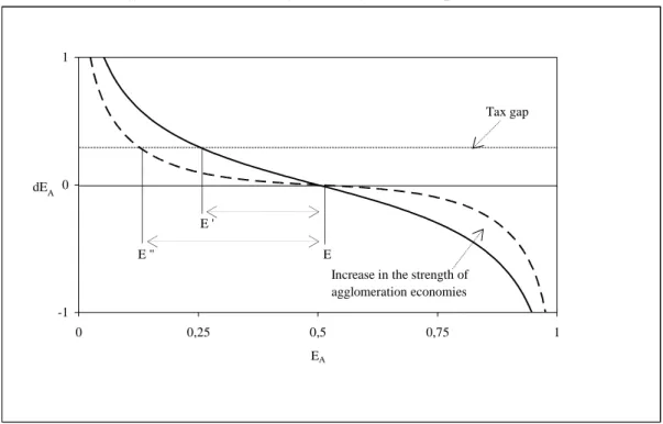
In Figures 2, 3, and 4 we illustrate how an increase in the strength of AE affects the impact of a given positive tax gap, T, on the allocation of entrepreneurs. Figure 2 depicts the case where a stable diversified symmetric equilibrium occurs. As can be observed, the stronger AE are, the larger the delocation of entrepreneurs is (E´´-E is larger than E´-E). Figure 3 deals with the case where, although a stable diversified equilibrium emerges, the endowment of land area makes jurisdiction A a much better location for running a business. In this case, stronger AE lead to smaller outflows of entrepreneurs (E´´´-E´´ is smaller than E-E´). Figure 4 deals with the case where a concentrated equilibrium emerges. In this case, it is also easily seen that stronger AE lead to smaller sensitivity to taxes on the part of firms.

Figure 2. The effect of an increase in the strength of AE on the sensitivity of entrepreneurs

to tax differentials in a diversified and symmetric equilibrium.

-1 0 1 0 0,25 0,5 0,75 1 EA dE_A E '' E E ' Tax gap

Increase in the strength of agglomeration economies

7

Burbidge et al. (2004) study tax competition in the presence of both AE and heterogeneity. They only comment on the impact of AE on the effects of taxes in the symmetric equilibrium.

Figure 3. The effect of an increase in the strength of AE on the sensitivity of entrepreneurs to tax differentials in a diversified equilibrium where entrepreneurs are highly concentrated in jurisdiction A.

-1 0 1 0 0,25 0,5 0,75 1 EA dE_A E' E E''' E'' Increase in the strength of

agglomeration economies

Tax gap

Figure 4. The effect of an increase in the strength of AE on the sensitivity of

entrepreneurs to tax differentials in a concentrated equilibrium where jurisdiction A is the core.

-1 0 1 0 0.25 0.5 0.75 1 EA dE_A E' E E''' E'' Tax gap

Increase in the strength of agglomeration economies

2.3

Testable predictions

Our theoretical results are derived in a 2-jurisdiction, 2-input and 1-good framework. This implies that meaningful testable predictions do not follow strictly from the results of the model. In our view, the main message of the theoretical analysis is that the effect of AE on the sensitivity of economic activities to local taxes hinges on the level of similarity in size across competing jurisdictions. As explained above, we consider municipalities to compete more intensely with their neighbors. Hence, our notion of competing municipalities is that of neighboring municipalities. Taking this into account we posit the following two testable predictions:

Testable prediction 1: A tax increase in jurisdiction i generates an outflow of economic

activity which increases with the strength of AE in municipality i if this jurisdiction is sufficiently similar to its neighbors in terms of the amount of economic activity hosted.

Testable prediction 2: A tax increase in jurisdiction i generates an outflow of economic

activity which decreases with the strength of AE in municipality i if this jurisdiction is sufficiently dissimilar to its neighbors in terms of the amount of economic activity hosted.

3.

Empirical analysis

3.1.Empirical specification

In this paper we examine the effects of local tax rates on the location of economic activities in equilibrium. AE may increase or decrease the effect of taxes because when a plant relocates it changes profit opportunities across locations. This implies that the effects we are interested in are cumulative in nature. Hence, looking at the individual location decisions of new and re-locating establishments (e.g., as in a conditional logit framework) does not seem appropriate in this particular context. Therefore, we define our dependent variable as an aggregate measure of economic activity. This could be either the number of firms or the number of employees in the municipality. There are a number of factors which, in practice and in the case of this particular analysis, lead us to prefer employment over the number of firms. First, note that there is no employment in the 2-input model introduced above. Since labour supply does not vary across municipalities within local labour markets, movements of firms and employees are conceptually equivalent. Entrepreneurs choose locations on the basis of profit differentials and workers

commute where job opportunities arise. Second, note also that taxes may have effects on both the extensive (plant births and re-locations) and intensive (plant contractions and production movements within multi-plant firms) margins8, suggesting that the aggregate effect might be best captured by employment. Finally, employment growth is the main aggregate economic variable to be found in the literature on the effects of taxes on economic activity (see, e.g., Bartik, 1991).

The baseline econometric model we consider is:

it t i it i it

emp

)

=

β

⋅

τ

+

α

+

α

+

ε

ln(

[11]

where empit denotes employment in municipality i at time t and

τ

_it is the local business tax rate. Note that employment is measured in logs. This reflects the fact that a unit increase in the tax rate is likely to generate larger effects on employment levels in large municipalities only because tax bases are larger. Thus, our main parameter of interest

β

_i measures the effect of the local tax rate on the percentage-change in employment.

α

_i is a municipal fixed-effect measuring time-invariant features that make jurisdiction i suitable for running a business. These features may include land availability, amenities, the presence of an international airport or access to transportation infrastructures. This municipal fixed-effect can also reflect history in terms of past levels of employment.

α

_t measures a year-specific effect which is common to all municipalities and may capture the state of the business cycle. Finally,

ε

_it denotes a year-municipal specific shock. First differencing equation [11] yields:

it t it i it

u

emp

=

⋅

Δ

+

+

Δ

ln(

)

β

τ

α

'

[12]

where

Δ

denotes the difference operator and u_it ≡ε_it−ε_it−k k being a positive integer. Due to the cumulative nature of the effects of taxes, changes in employment have to be measured in a window of time which has to be long enough to enable the effects of interest to show up, i.e. k has to be large enough. Since the change in employment measured in logs is closely related to the employment growth rate, we use municipal employment growth to refer to our dependent variable.

8

For example, Gobillon et al. (2007) find that taxes affect plant size (extensive margin) but not new plant location (extensive margin).

Our main goal is to investigate the way in which

β

_i varies across municipalities. For that purpose we introduce a measure of the strength of AE at the municipal level,

γ

_i. We also introduce a measure of the dissimilarity in size between a jurisdiction and its neighbors,

μ

_i. We turn to the definition of these variables in the next section. Our empirical strategy relies on allowing the local tax rate effect to be a function of the AE and dissimilarity measures at the initial time period. We posit the following functional form for

β

_i:

k it k it k it i

≡

β

+

β

⋅

γ

−

+

β

⋅

γ

−

⋅

μ

−

β

1 2 3 [13]

where

β

₁,

β

₂ and

β

₃ are parameters to be estimated. The effect of an increase in the strength of AE on the effect of taxes is seen by differentiating

β

_i with respect to

γ

_it−k:

k it k it i

d

d

− −

⋅

+

=

β

β

μ

γ

β

3 2 [14]

We expect

β

2

+

β

3

⋅

μ

_it−k to be negative when the degree of similarity between jurisdiction i and its neighbors,

μ

_it−k, is low enough (Testable prediction 1). Instead we expect

k it−

⋅

+

β

μ

β

2 3 to be positive when jurisdiction i is sufficiently dissimilar to its neighbors, i.e. k

it−

μ

is high enough (Testable prediction 2). For this to be the case

β

₃ has to be positive (

β

3

>

0

) whereas no particular sign is expected for

β

2.

3.2. Data and variables

Data: The empirical analysis is carried out with municipal data for the period 1995-2002. The sample is restricted from the outset to the 946 municipalities of Catalonia, a region in north-east Spain9. The analysis is restricted to Catalonia as employment data for this period are not available to researchers for all the Spanish municipalities, with the exception of the year 2002, which we use in some of our calculations (see below). Employment data at the municipal level are drawn from the Social Security Register database. These data are available at the 2-digit

9

In 2002, the local business tax was reformed and from 2003 onwards municipal tax rates were no longer comparable with those set in previous years.

level of sectoral detail which yields 49 industries10. Unfortunately, the analysis could not be carried out with all municipalities in the region due to data availability. Specifically, tax rates are only available for municipalities exceeding 5,000 inhabitants in 1995, 1,000 inhabitants between 1996 and 1999 and all municipalities from 2000 onwards. This means that we are able to use 256 municipalities for the first period, and 419 for the second, making a total of 675 observations. As discussed in section 3.1, the effects we are looking at are cumulative and therefore we are not interested in one-year time changes. Since municipal elections were held in 1995 and 1999 and tax rates for year t are decided at the end of t−1 we examine the two non-overlapping three-year periods, namely Dec. 1995 to Dec. 1998 and Dec. 1999 to Dec. 2002. Hence, we use the variation in tax rates that occurred during the first three term-of-office years, implying k=3. In Table 1 descriptive statistics of the data are provided11.

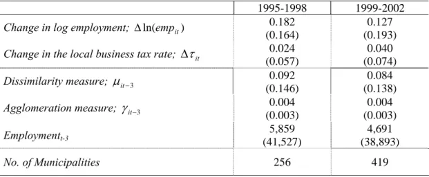
Table 1. Summary statistics by sub-periods.

1995-1998 1999-2002 Change in log employment; Δln(emp_it) 0.182

(0.164)

0.127 (0.193) Change in the local business tax rate;

Δ

τ

_it 0.024

(0.057) 0.040 (0.074) Dissimilarity measure;

μ

_it−3 0.092 (0.146) 0.084 (0.138) Agglomeration measure;

γ

_it−3 0.004 (0.003) 0.004 (0.003) Employmentt-3 _(41,527) 5,859 _(38,893) 4,691 No. of Municipalities 256 419

Local taxes: The size of Spanish municipal governments is moderate, with municipal budgets representing 15% of total public spending. Inter-governmental grants represent a third of local budgets while local taxes represent another third and the remainder consist of user charges. The business sector is charged a number of municipal taxes and fees. This list includes a local business tax, a property tax, a tax on vehicles, a tax on building activities, and a tax on the sale of land and buildings. Although the property tax (Impuesto sobre la propiedad immueble) comes first in terms of tax revenue, the local business tax (Impuesto sobre Actividades

10

The Spanish 2-digit classification (CNAE 93) currently comprises 60 industries. However, in 1995 a different classification was used (CNAE 74). In order to make these data comparable industries have to be aggregated yielding 49 economic sectors.

11

Note that a longer window (e.g., k=6) would have impeded the control for period-specific common shocks, which seem to be relevant in our case (see section 3).

Económicas) is the main local tax burden borne by the business sector12. Jofre-Monseny and Solé-Ollé (2007) reported that the effect of the local business tax on the location of new establishments outweighed that of the property tax by a factor of 4. No effect was found for the remaining local taxes or for spending.

The local business tax liability of each firm is based on a presumed level of profits. This presumed level of profits is determined by national tax laws according to input usages and the economic sector of the firm. This presumed level of profits is the modified at the municipal level at being multiplied by a municipal tax rate,

τ

_i. Hence, differences in business tax rates mean that firms pay different shares of their profits in different municipalities. Municipal governments are given quite considerable tax autonomy and local business statutory tax rates can vary from 0.8 to 1.9. However, the range within which municipalities can set their tax rate varies with population size. The maximum tax rate increases from 1.4 (<5,000 inhabitants) to 1.6 (5,001-20,000 inhabitants), to 1.7 (20,001-50,000 inhabitants), to 1.8 (50,001-100,000 inhabitants) and to 1.9 (>100,0000 inhabitants). In Figure 5 we plot the local business tax rate against population for all municipalities whose population exceeds 1,000 inhabitants in 199913. Instead, the minimum tax rate is 0.8 for all municipalities.

12

For a more detailed description of local business taxation in Spain see Jofre-Monseny and Solé-Ollé (2007).

13

Figure 5. Scatter plot of business tax rates vs. population in 1999. Legal maximum business tax rates jump at 5, 20, 50 and 100 thousand inhabitants.

0.7 0.8 0.9 1 1.1 1.2 1.3 1.4 1.5 1.6 1.7 1.8 1.9 2 1 5 20 50 100

Inhabitans (in thousands)

Note that the variation in statutory tax rates is considerable. Note too, that the number of municipalities that set a tax rate that is equal to the maximum permitted by law is 36%. Besides, from 1996 to 2002, for municipalities with at least 1,000 inhabitants, the share of municipalities whose maximum tax rate was binding increased from 32% to 42%14. This reflects the fact that local business tax rates increased over the period studied.

The strength of AE in municipality i: We identify variation in the strength of AE across municipalities from two sources: 1) Variation in the strength of AE across industries; 2) Variation in the industry mix across municipalities. Thus, a municipality in which industries with high AE are over-represented is classified as a municipality with strong AE. Differences in the strength of AE across industries are identified from differences in the geographic concentration of industries. The Ellison-Glaeser agglomeration index (1997) is a well-established measure of the geographic concentration of an industry. This index measures the extent to which an industry is geographically concentrated while controlling for: 1) The

14

Note that our analysis is restricted to municipalities with at least 1,000 inhabitants. We do not have information on all municipalities in 1995 with a population between 1,000 and 5,000 inhabitants. Therefore we undertake a comparison between 1996 and 2002.

geographic concentration of the economic activity in general; 2) The fact that industries differ in their industrial organization15. This index can be understood as a measure of the tendency of plants within an industry to co-locate in space. Therefore, it can be considered a measure of the strength of AE within one industry. Ellison and Glaeser (1997) also proposed a agglomeration index, which computes the tendency of plants from different industries to co-locate in space. The co-agglomeration index measures the strength of AE across industries. Plant-level data are required to compute Ellison-Glaeser indices. Following Guimarães et al. (2007), here we construct our indices using data from plant-counts16. These authors show that plant-count data and the original Ellison-Glaeser versions of the index yield the same expected value. Besides, the variance of the index is smaller using plant-count data. We compute a 49

×

49 matrix of agglomeration and co-agglomeration indices. The element

γ

m,n measures the strength of AE between firms of the mth and nth industries. If m=n then the co-agglomeration index is just the agglomeration index for the mth industry. These pair wise indices are computed using data from all continental Spanish municipalities for the year 2002. We propose the following measure of the strength of AE in municipality i:

∑∑

∀ ∀

⋅

=

m n n m i i

p

m

n

,

)

,

(

γ

γ

[15]

where

p

_i

(

m

,

n

)

stands for the probability that on drawing two employees randomly from municipality i, one will belong to industry m and the other to industry n. The probability

)

,

(

m

n

p

_i can be written as:

∑

∑

⋅

=

n i in m i im i

emp

emp

emp

emp

n

m

p

(

,

)

[16]

where empim and empin denote the employment levels of the mth and nth industry in municipality i. Note that

γ

_i captures the extent to which industries (and pairs of industries) with high AE are over-represented in a municipality.

15

Note that an industry which comprises a small number of plants will necessarily be highly concentrated spatially.

16

This implies that: 1) the share of plants in each industry is used instead of the share of employment in each industry; 2.) the Hirschmann-Herfindahl index for each industry is replaced by 1 over the sum of plants in each industry.

Dissimilarity between jurisdiction i and its neighbors: Testable predictions 1 and 2 imply that the effect of AE on the sensitivity of economic activity to taxes depends crucially on the way in which jurisdiction i relates to its neighbors in terms of size. We consider two municipalities to be neighbors if they belong to the same local labor market17. The proposed measure of dissimilarity between municipality i and its neighbors is:

∑

∈

−

⋅

−

=

l j i j l i

abs

s

s

N

1

(

)

1

μ

[17]

where

N

_l is the number of municipalities that constitute local labor market l and

s

_i and

s

_j are the shares of municipalities i and j in the employment of local labor market l. Hence, expression [16] is the expected difference in employment shares between municipality i and a jurisdiction drawn randomly from its local labor market18.

In Catalonia, and elsewhere, the municipality size distribution is highly skewed to the right. Hence, our dissimilarity measure,

μ

_i, will typically be high for the largest municipality in the local labor market which often acts as a central business district. For the remaining municipalities the dissimilarity measure will typically be low. This is so because small municipalities, as opposed to their larger counterparts, tend to have many neighbors that are similar in size. Hence, although economic activities are highly concentrated in space, most jurisdictions compete with many similarly sized neighbors.

3.3. Ordinary Least Squares (OLS) estimates

Endogeneity is the main econometric concern when estimating the effect of local taxes on the location of economic activities. More specifically, we are particularly concerned that shocks in employment might be correlated to changes in tax rates, given that municipal authorities may alter these rates in response to shocks in municipal employment. Suppose a left-wing mayor sees that a large plant abandons her municipality. She may then come under some pressure to

17

The local labour markets to which we refer have been computed by Roca and Moix (2004). Municipalities are aggregated in groups according to commuting considerations. Broadly speaking, each local labour market is built to ensure people live and work within its boundaries. Thus, the 946 municipalities make up 41 local labour markets. With this level of aggregation, approximately 75% of the people live and work in the same local labour market.

18

We have used other variables to capture dissimilarity in terms of size. For instance, we have computed expected differences in employment levels instead of differences in employment shares. We have also used other notions of geographic neighborhood (inverse distance weighting instead of using the binary notion of belonging to the same local labor market). The results obtained when using these alternative measures of dissimilarity remain largely unchanged.

cut taxes and she may do so which implies that

cov(

ε

_it−3

,

τ

_it

)

≠

0

. Hence,

u

_it

≡

ε

_it

−

ε

_it−3 may be correlated to

Δ

τ

_it and OLS estimates of the effects of taxes on employment growth may be biased19. One way to attenuate this endogeneity bias is to introduce controls for the different shocks that might affect municipalities within the region asymmetrically. In order to control for shocks that may be specific to small geographic areas within the region, we introduce

×

year

local labor market fixed effects. From a conceptual point of view, this step is highly significant to our analysis. Note that the inclusion of these fixed effects amounts to exploit the variation in tax rates that arises within local labor markets. This fits with our notion that neighboring jurisdictions compete more intensely over tax bases. Municipalities in which industries experiencing decline are over-represented may experience little growth. To control for industry mix related shocks we construct the following variable:

∑

∑

∑

⎟

⎟

⎟

⎠

⎞

⎜

⎜

⎜

⎝

⎛

⎟⎟

⎠

⎞

⎜⎜

⎝

⎛

Δ

⋅

=

n i n it

emp

emp

emp

emp

int int int int

η

[18]

which is no more than the employment growth that municipality i would experience if every industry in i grew at the same rate as that experienced by the industry at the regional level. Finally, we also introduce the initial employment level to capture mean reverting behavior.

Although these controls can explain a considerable degree of variation in employment growth across municipalities, their inclusion as control variables is not likely to eliminate the endogeneity bias completely. However, note that our main object of interest is not the average effect of taxes. This enables us to take a difference-in-difference sort of approach. Recall our baseline econometric specification20:

it it it it it it it it

u

emp

=

⋅

Δ

+

⋅

Δ

⋅

+

⋅

Δ

⋅

⋅

+

Δ

ln(

)

β

₁

τ

β

₂

τ

γ

₋₃

β

₃

τ

γ

₋₃

μ

₋₃ [19]

Note that we can right the linear projection of

u

_it onto the observables in equation [19] in error form as:

19

Note that

ε

_it−3 is, in principle, uncorrelated to

τ

_it−3 since the latter is set at the end of

τ

_it−4.

20

For the sake of simplicity we do not include a constant term (or any local labor market dummies) or the other controls in equations [19], [20] and [21]. Our argument also holds when these variables are included.

it it it it it it it it

u

=

δ

₁

⋅

Δ

τ

+

δ

₂

⋅

Δ

τ

⋅

γ

₋₃

+

δ

₃

⋅

Δ

τ

⋅

γ

₋₃

⋅

μ

₋₃

+

υ

[20]

where

υ

_it is an error term. If we plug expression [20] into [19] we obtain:

it it it it it it it it emp =

β

+

δ

⋅Δ

τ

+

β

+

δ

⋅Δ

τ

⋅

γ

+

β

+

δ

⋅Δ

τ

⋅

γ

⋅

μ

+

υ

Δln( ) ( _{1 1}) ( _{2 2}) ₋₃ ( _{3 3}) _{−3 −3} [21]

Note that

υ

_it is uncorrelated to all variables in this equation by construction. Hence, unbiased estimates of

β

₂ and

β

₃ can be obtained through an OLS regression of equation [21] as long as

0

2 =

δ

and

δ

3

=

0

. Hence, our identifying assumption is that governments change tax rates according to shocks in employment regardless of the values that the AE and dissimilarity measures take. Given the possibility that the AE and dissimilarity measures (

γ

it−3 and

μ

it−3) may be correlated to employment shocks,

u

_it, it is necessary to check that OLS estimates of equation [21] are robust to the inclusion of

γ

it−3 and

γ

it−3

⋅

μ

it−3 as separate control variables. OLS results: In Table 2 we present the OLS estimates of the equation in which we are interested. Both the agglomeration and the dissimilarity measures have been standardized to a mean value of zero and a standard deviation of one. All estimations include

year

×

local labor market fixed effects. Specifications [2], [3] and [4] include the employment level at the base year. Specifications [3] and [4] also include the variable measuring industry mix shocks, i.e.

it

η

. Specification [4] includes additionally

γ

_it−3 and

γ

_it−3

⋅

μ

_it−3 as separate control variables. In all specifications, F-tests of year× local labor market vs. year effects reject the hypothesis that fixed effects do not vary across local labor markets for a given year. The employment level at the base year is found to exert a negative effect on municipal employment growth. In its turn, the variable measuring the industry mix shock for municipality i,

η

_it is statistically significant and takes the expected sign and order of magnitude. The control variables

γ

_it−3 and

γ

_it−3

⋅

μ

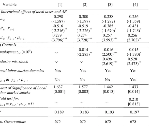
_it−3 are jointly not significantly different from zero. In light of these results, we consider specification [3] to be our preferred specification. Note, however, that our results regarding the effects of taxes do not undergo any significant changes across specifications.

Table 2. The effects of changes in tax rates on changes in employment (in logs). Changes defined over a three-year period. Pooled observations from 1995-1998 & 1999-2002. OLS estimates.

Variable [1] [2] [3] [4]

i) Intertwined effects of local taxes and AE

-0.298 -0.300 -0.238 -0.256 it

τ

Δ

(-1.587) (-1.597) (-1.292) (-1.359) -0.516 -0.519 -0.385 -0.431 3 −

⋅

Δ

τ

_it

γ

_it (-2.216)** (-2.226)** (-1.670)* (-1.743)* 0.279 0.274 0.257 0.256 3 3 − −

⋅

⋅

Δ

τ

_it

γ

_it

μ

_it (3.796)*** (3.728)*** (3.593)*** (2.702)** ii) Controls -0.014 -0.016 -0.015 Employmentt-3(×105) -.- (-2.283)** (2.500)*** (-1.780)* 0.496 0.528

Industry mix shock -.- -.-

(2.619)*** (2.473)**

Local labor market dummies Yes Yes Yes Yes

3 3 3

&

− − − it

⋅

it it

γ

μ

γ

No No No Yes 1.637 1.577 1.442 1.433 F-test of Significance of Local

labor market shocks [0.001] [0.003] [0.013] [0.014]

Wald test for:

0

3 3 3

=

−

⋅

−

=

− it it it

γ

μ

γ

-.- -.- -.- 0.210 [0.813] R2 0.189 0.183 0.193 0.197 No. Observations 675 675 675 675

Notes: 1. Figures in parentheses are robust standard errors. 2.*,**,*** denotes significance at 1, 5 and 10% level. Figures within brackets are p-values.

As explained above, the OLS estimate of

β

₁, measuring the average effect of a rise in taxes, is most likely to be biased. Hence, we focus here on the interaction terms between taxes and the AE and dissimilarity measures. Most importantly,

β

3 is positive and statistically different from zero. This is consistent with testable predictions 1 and 2 above. Given the point estimates of

β

₂ (-0.385) and

β

₃ (0.257) obtained in specification [3], we can obtain the threshold that solves

0

3 3

2

+

β

⋅

μ

it−

=

β

. This threshold is 1.5. This implies that AE reduce the effect of taxes if

μ

it−3 is, at least, 1.5 standard deviations larger than the mean. The opposite is the case for dissimilarity levels below this threshold. Around 14% of our sample shows a dissimilarity measure above 1.5 standard deviations. This implies that for most of our sample stronger AE imply the more marked effect of taxes. This can be explained by the fact that most municipalities are small and generally compete with many similarly sized neighbors.

3.4. Instrumental variables (IV) estimates

Obtaining a reliable estimate of the average effect of tax rate changes on employment growth, i.e.

β

₁, is interesting in itself but, above all, it enables us to place the estimates of

β

₂ and

β

₃ in context. That is, in order to know the extent to which AE influence the effect of taxes, we need an estimate of the average effect of the variable of interest. This calls for an instrumental variables approach which requires some exogenous variation in local business tax rates.

Instruments: The source of exogenous variation we rely on comes from a particular institutional characteristic of Spain’s local business tax: namely, that there are legal limits on maximum tax rates which vary across municipalities discretely according to population size (See section 3.2 and Figure 5). Here, we aim at using the maximum taxate as an instrumental variable for the tax rate change.

The first requirement an instrumental variable has to satisfy is that it must shift the variable of interest. Data on local business tax rates present two important features in this respect, highlighted above in section 3.2. First, the share of municipalities whose maximum tax rate is binding is not low (30-40% range). Second, local business tax rates increased during the period 1995-2002. As a result, the share of municipalities whose maximum tax rate is binding also increased during this same period (from 32% to 42%). For most municipalities with binding maximum tax rates, the decision to change tax rates is obviously a constrained one. Hence, maximum tax rates are very likely to determine in part tax rate choices as well as their changes. For non-binding municipalities, maximum tax rates can partly determine tax setting behavior, too. For instance, municipal governments may be reluctant to choose the maximum tax rate level, or one which is too close to it, since this leaves them with no room for maneuver in case of future budget difficulties. Hence, the assumption that maximum tax rates shift tax rate changes seems a plausible one. Note that this is a testable assumption and one that we examine below.

The second requirement for an instrumental variable is that it should be uncorrelated to the error term. In our case this means that maximum tax rates should be uncorrelated to shocks in employment growth. Maximum tax rates are not exogenous since they vary with population size. However, we claim that maximum tax rates are uncorrelated to shocks in employment growth conditional on the employment level in the base year, year×local labor market fixed effects and our variable capturing industry mix related shocks. Our maintained assumption is

that these controls will absorb any correlation between population size and shocks in employment growth.

The maximum tax rate may not be the only instrumental variable this particular institutional set-up may generate. For instance, another candidate instrument is the distance to the maximum tax rate (

τ

_itMax

−

τ

_it−3). It is reasonable to think that it is this distance and not the maximum tax rate itself that determines the tax rate setting behavior. However, a gain in terms of increasing the capacity to shift taxes may come at the cost of decreasing our confidence that the instrument is uncorrelated to shocks in employment. Suppose that shocks in employment are serially correlated, i.e.

cov(

ε

it

,

ε

it−1

)

≠

0

. A negative shock in t−4 may lead to a tax increase in t−3 and hence

τ

it−3 may be correlated to

ε

it−3 if

cov(

ε

it−4

,

ε

it−3

)

≠

0

. Thus

τ

itMax

−

τ

it−3 may not be a valid instrument in the sense that it can be correlated to

u

_it

≡

ε

_it

−

ε

_it−3 through

ε

_it−4. However, we can use the interaction term between the distance to the maximum and being a left-wing government, i.e.

(

τ

_itMax

−

τ

_it−3

)

⋅

left

21

. The idea is that left-wing governments set higher tax rates than their right-wing counterparts. In fact, the share of left-wing governments whose maximum tax rates are binding is remarkably higher. In 1999, this share was 42% for left-wing governments and 25% for right-wing governments. Hence, conditional on a given distance to the maximum (τitMax−τit−3) being a left-wing government may generate an extra boost in terms of expected tax rate increases which can be considered to be uncorrelated to shocks in employment growth.

Instrumental variables results: We now turn to the data to assess the degree to which: 1) The instrument shifts the endogenous variable (the model is identified); 2) There are any grounds to suspect that the instruments are correlated with the error term. We focus this discussion on estimating an average effect of tax rate increases on employment growth. That is, we leave out, for the time being, the interaction terms between tax rate changes and the AE and dissimilarity measures. Columns 1 and 3 report first and second stage estimates when the only excluded instrument used is the maximum tax rate (

τ

_itMax). Columns 2 and 4 report the results obtained when both

τ

_itMax and the interaction term

(

τ

_itMax

−

τ

_it−3

)

⋅

left

are used as excluded instruments.

21

By left-wing government we refer to governments whose mayor belongs to the Socialist Party (PSC/PSOE) or the Green Party (IC/IU). The share of left-wing governments was 34% in Dec. 1995-Dec. 1998 and fell to 27% in Dec. 1999-Dec. 2002.

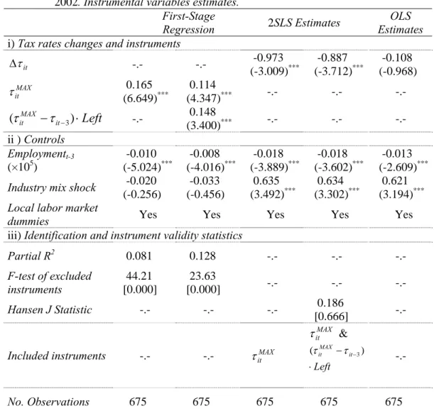
Table 3. The effects of changes in tax rates on changes in employment (in logs). Changes defined over a three-year period. Pooled observations from 1995-1998 & 1999-2002. Instrumental variables estimates.

First-Stage

Regression 2SLS Estimates

OLS Estimates i) Tax rates changes and instruments

-0.973 -0.887 -0.108 it τ Δ -.- -.- (-3.009)*** (-3.712)*** (-0.968) 0.165 0.114 MAX it τ (6.649)*** (4.347)*** -.- -.- -.- 0.148

Left

it MAX it

−

−

)

⋅

(

τ

τ

₃ -.- (3.400)*** -.- -.- -.- ii ) Controls -0.010 -0.008 -0.018 -0.018 -0.013 Employmentt-3 (×105) (-5.024)*** (-4.016)*** (-3.889)*** (-3.602)*** (-2.609)*** -0.020 -0.033 0.635 0.634 0.621 Industry mix shock

(-0.256) (-0.456) (3.492)*** (3.302)*** (3.194)*** Local labor market

dummies Yes Yes Yes Yes Yes

iii) Identification and instrument validity statistics

Partial R2 _{0.081 0.128 -.- -.- -.-} F-test of excluded instruments [0.000] 44.21 23.63 [0.000] -.- -.- -.- Hansen J Statistic -.- -.- -.- 0.186 [0.666] -.-

Included instruments -.- -.- τ_itMAX

MAX it τ & Left it MAX it ⋅ − ₋ ) (τ τ ₃ -.- No. Observations 675 675 675 675 675

Notes: 1. Figures in parentheses are robust standard errors. 2.*,**,*** denotes significance at 1, 5 and 10% level. 2. Figures within brackets are p-values.

First-stage regression results show that both the maximum tax rate,

τ

_itMax and the interaction term

(

τ

_itMax

−

τ

_it−3

)

⋅

left

are statistically significant determinants of tax rate changes. The F-test of excluded instruments takes a value which is above 20 in both cases22. Hence, the instruments proposed seem to shift tax rate changes. Note that the partial R2 increases from 8 to 12% when including

(

τ

_itMax

−

τ

_it−3

)

⋅

left

as an excluded instrument.

We now turn to the second-stage results. The last column of the table shows the OLS results for comparative purposes. The 2SLS estimates of the effect of taxes on employment growth are

22

Staiger and Stock (1997) suggest, as a rule of thumb, that an F-test below 10 may be associated with weak instrument problems.

negative and statistically different from zero. The effect is -0.973 when only

τ

_itMax is used and -0.887 when both

τ

_itMax and

(

τ

_itMax

−

τ

_it−3

)

⋅

left

are used. This implies that a municipality that increases its business tax rate one standard deviation below the average increases municipal employment growth by approximately 5% over a three-year period. Note that the estimate obtained by OLS is -0.108 indicating the need for instrumental variables estimation. The assumption that the maximum tax rate is uncorrelated to employment shocks is not testable when only

τ

_itMax is used as an instrument. However, when both

τ

_itMax and

(

τ

_itMax

−

τ

_it−3

)

⋅

left

are used, a test of over-identifying restrictions can be computed. The Hansen J statistic takes a low value and, as such, does not raise concerns about the validity of the instruments.

Thus, we obtained OLS estimates for the interaction terms between local taxes and AE which are unbiased under plausible assumptions in section 3.3 and, above, we also obtained an instrumental variables estimate of an average effect of local taxes on employment growth. We now aim at obtaining joint estimates of all these parameters. A conservative approach would be to instrument all variables containing tax rate changes, i.e.,

Δ

τ

_it,

Δ

τ

_it

⋅

γ

_it−3 and

3

3 −

−

⋅

⋅

Δ

τ

_it

γ

_it

μ

_it . Instruments for the interaction terms are simply obtained by interacting

γ

it−3 and

γ

it−3

⋅

μ

it−3 with instruments

Max it

τ

and

(

τ

_itMax

−

τ

_it−3

)

⋅

left

23

. The results of this exercise are reported in the first column of Table 4.

23

The Kleibergen-Paap rk LM statistic provided by the Stata command ivreg2 rejects the hypothesis that the model is unidentified. Note that the F-test of excluded instruments can be misleading in the case where several variables are endogenous.

Table 4. The effects of changes in tax rates on changes in employment (in logs). Changes defined over a three-year period. Pooled observations from 1995-1998 & 1999-2002. Instrumental variables estimates.

[1] [2] [3]

i) Intertwined effects of local taxes and AE

-0.886 -0.886 -0.863 it τ Δ (-1.834)* (-1.842)* (-3.534)*** -0.336 -0.336 -0.375 3 −

⋅

Δ

τ

_it

γ

_it (-0.704) (0.717) (-2.245)** 0.151 0.151 0.224 3 3 − −

⋅

⋅

Δ

τ

_it

γ

_it

μ

_it (1.636) (1.750)* (3.582)*** ii ) Controls -0.017 -0.017 -0.016 Employmentt-3(×105) (-3.275)*** (-3.023)*** (-3.353)*** 0.522 0.522 0.509 Industry mix shock

(2.140)** (2.106)** (2.961)***

Local labor market dummies Yes Yes Yes

iii) Instrumented variables it τ Δ Yes -.- Yes 3 −

⋅

Δ

τ

_it

γ

_it &

Δ

τ

it

⋅

γ

it−3

⋅

μ

it−3 Yes -.- No iv) Hausman Endogeneity test

0.708 ≡ 1 v Δτ_it -.- (1.438) -.- ≡ 2 v

Δ

τ

it

⋅

γ

it−3 -.- _(-0.384) -0.186 -.-

≡

3

v

Δ

τ

it

⋅

γ

it−3

⋅

μ

it−3 -.- _(0.977) 0.122 -.- 3.41 Wald-test

v

₁

=

v

₂

=

v

₃

=

0

-.- [0.017] -.- 0.48 Wald-test

v

₂

=

v

₃

=

0

-.- [0.618] -.- No. Observations 675 675 675

Notes: 1. Figures in parentheses are robust standard errors. 2.*,**,*** denotes significance at 1, 5 and 10% level. 2. Figures within brackets are p-values. 3. Excluded instruments are τ_itMAXand

Left

it

MAX

it

−

−

)

⋅

(

τ

τ

3 and their interactions with

γ

it−3 &

γ

it−3

⋅

μ

it−3 in all regressions. 4.-Upper-bar variables denote first stage fitted values.

Note that the estimate we obtain for

β

1 (-0.886), which measures the effect of a tax change for a municipality with average AE and dissimilarity measures, is very similar to the estimate obtained when the AE and