Semisupervised Hypergraph Discriminant Learning
for Dimensionality Reduction of Hyperspectral Image
Fulin Luo
, Member, IEEE
, Tan Guo
, Zhiping Lin
, Senior Member, IEEE
,
Jinchang Ren
, Senior Member, IEEE
, and Xiaocheng Zhou
Abstract—Semisupervised learning is an effective technique to represent the intrinsic features of a hyperspectral image (HSI), which can reduce the cost to obtain the labeled information of sam-ples. However, traditional semisupervised learning methods fail to consider multiple properties of an HSI, which has restricted the discriminant performance of feature representation. In this article, we introduce the hypergraph into semisupervised learning to reveal the complex multistructures of an HSI, and construct a semisu-pervised discriminant hypergraph learning (SSDHL) method by designing an intraclass hypergraph and an interclass graph with the labeled samples. SSDHL constructs an unsupervised hypergraph with the unlabeled samples. In addition, a total scatter matrix is used to measure the distribution of the labeled and unlabeled sam-ples. Then, a low-dimensional projection function is constructed to compact the properties of the intraclass hypergraph and the unsupervised hypergraph, and simultaneously separate the charac-teristics of the interclass graph and the total scatter matrix. Finally, according to the objective function, we can obtain the projection matrix and the low-dimensional features. Experiments on three HSI data sets (Botswana, KSC, and PaviaU) show that the proposed method can achieve better classification results compared with a few state-of-the-art methods. The result indicates that SSDHL can
Manuscript received May 20, 2020; revised July 6, 2020; accepted July 20, 2020. Date of publication July 23, 2020; date of current version August 7, 2020. This work was supported in part by the National Natural Science Foundation of China under Grant 61801336, in part by the China Postdoctoral Science Foundation under Grant 2019M662717, in part by the Fundamental Research Funds for the Central Universities under Grant 2042020kf0013, in part by the Science and Technology Major Project of Hubei Province (Next-Generation AI Technologies) under Grant 2019AEA170, in part by the Science, and Technology Research Program of the Chongqing Municipal Education Commission under Grant KJQN201800632, in part by the Open Research Fund of State Key Labo-ratory of Integrated Services Networks under Grant ISN20-12, in part by Open Research Project of the Hubei Key Laboratory of Intelligent Geo-Information Processing under Grant KLIGIP-2018A06, and in part by the Open Research Fund of Key Laboratory of Spatial Data Mining, and Information Sharing of Ministry of Education, Fuzhou University, under Grant 2019LSDMIS06. (Corresponding author: Tan Guo.)
Fulin Luo is with the State Key Laboratory of Information Engineering in Surveying, Mapping, and Remote Sensing, Wuhan University, Wuhan 430079, China (e-mail: [email protected]).
Tan Guo is with the School of Communications and Information Engineering, Chongqing University of Posts and Telecommunications, Chongqing 400065, China (e-mail: [email protected]).
Zhiping Lin is with the School of Electrical and Electronic Engi-neering, Nanyang Technological University, Singapore 639798 (e-mail: [email protected]).
Jinchang Ren is with the Department of Electronic and Electrical Engineering, University of Strathclyde, G11XW Glasgow, U.K. (e-mail: [email protected]).
Xiaocheng Zhou is with the Key Laboratory of Spatial Data Mining and Information Sharing of Ministry of Education, Fuzhou University, Fuzhou 350116, China (e-mail: [email protected]).
Digital Object Identifier 10.1109/JSTARS.2020.3011431
simultaneously utilize the labeled and unlabeled samples to repre-sent the homogeneous properties and restrain the heterogeneous characteristics of an HSI.
Index Terms—Dimensionality reduction (DR), graph learning, hyperspectral image (HSI) classification, locality-constrained linear coding, neighborhood margin.
I. INTRODUCTION
A
HYPERSPECTRAL image (HSI) is composed of tens or hundreds of consecutive narrow electromagnetic bands covering the visible-to-infrared spectrums [1], [2]. Due to the abundant spectral and spatial information of an HSI, it can be used to discriminate different types of land covers [3], [4]. Generally, an HSI covers a large region. Machine learning is an effective way to automatically discriminant the land cover types of HSI [5], [6]. For the high-dimensional structure of HSI data, traditional recognition methods face the challenge of the Hughes phenomenon [7], [8]. To address this challenge, the dimensionality reduction (DR) of HSI data becomes crucial.In the past decades, DR has been widely used to process high-dimensional data, which reduces the dimensionality of data via transforming high-dimensional data into a low-dimensional space while preserving the useful information as much as possible [9], [10]. The classic DR methods include principal component analysis (PCA) and its variations [11], [12], linear discriminant analysis (LDA) [13], and maximum noise fraction (MNF) [14]. These methods utilize the variance property of the data to construct a DR model. Specifically, PCA maximizes the variance of the orthogonal projection of data, LDA considers the within-class and between-class variance, and MNF utilizes the noise variance to construct the projection model. However, these methods only consider the statistical properties, which neglect the intrinsic structures of the data. To better analyze the intrinsic properties of the data, manifold learning has been developed to reveal the geometry structures of the data [15], [16]. Some representative algorithms include isometric mapping (Isomap) [17], locally linear embedding (LLE) [18], and Lapla-cian eigenmaps (LE) [19]. These methods consider a certain local properties to describe the intrinsic manifold of the high-dimensional data in a low-high-dimensional space while the three methods belong to nonlinear projection that cannot obtain spe-cific projection matrix to map the out-of-sample into the corre-sponding low-dimensional space. To address this out-of-sample extension problem, LLE and LE are linearized to neighborhood This work is licensed under a Creative Commons Attribution 4.0 License. For more information, see https://creativecommons.org/licenses/by/4.0/
preserving embedding (NPE) [20] and locality preserving pro-jections (LPP) [21], respectively. To generalize these methods, a unified graph framework was developed to represent these DR models [22]. This framework considers a certain statistic or geometry properties to construct a graph model. Thus, according to different statistic or geometry characteristics, different graph learning algorithms can be designed with various construction manners of similarity matrix and constraint matrix. Based on the view of graph framework, many advanced methods have been developed to better reveal the intrinsic properties of the data, such as marginal Fisher analysis (MFA) [22], local Fisher dis-criminant analysis (LFDA) [23], regularized local disdis-criminant embedding (RLDE) [24], and local geometric structure Fisher analysis (LGSFA) [25].
The above-mentioned methods are unsupervised or super-vised models. For these unsupersuper-vised methods, they do not use any prior information to construct the low-dimensional feature learning models. For these supervised methods, they need to know the label information of the training samples to design the DR models. In real-world applications, an unsuper-vised technique cannot achieve desired performance in general, whereas supervised algorithms usually require a high cost to obtain the labeled information for the training samples [26]. To enhance the discriminant performance or reduce the cost of labeling samples, semisupervised learning was proposed to simultaneously utilize the labeled and unlabeled samples to con-struct the DR models [27], [28]. Based on the margin criterion, a semisupervised maximum margin criterion (SSMMC) [29] was proposed to improve the margin discriminant power of different classes. According to the theory of graph learning, semisupervised graph learning (SEGL) [30] was designed to build a semisupervised graph with the labeled and unlabeled samples. Meanwhile, LDA was used to develop semisupervised discriminant analysis (SDA) [31] and semisupervised local discriminant analysis (SELD) [32]. In addition, two semisu-pervised methods, i.e., semisusemisu-pervised submanifold preserving embedding (S3MPE) [33] and semisupervised sparse manifold discriminative analysis (S3MDA) [34], consider the manifold structures of the data to enhance the representation of intrinsic characteristics.
These traditional graph learning methods only consider the binary relationship between the sample points; hence, they show relatively unrealistic performance on an HSI due to the complex multiple structures it contains. Generally, the traditional graph is difficult to represent the intrinsic high-order relationships of HSIs. To reveal multiple properties of the data, hypergraph was introduced into the field of machine learning [35]–[37]. In hypergraph, each hyperedge contains more than two vertices, whereas the traditional graph just has two vertices on each edge [38], [39]. Subsequently, a series of hypergraph learning methods have been developed for DR of the data. Accord-ing to LPP, a binary hypergraph (BH) [40] was proposed to extract the features of an HSI. In addition, a supervised hy-pergraph learning method was proposed to improve the rep-resentation performance of low-dimensional features, termed discriminant hyper-Laplacian projection (DHLP) [41]. For an HSI, the spatial-spectral information was used to construct different spatial-spectral hypergraph models, including spatial
hypergraph (SH) [40], hypergraph embedding based spatial-spectral joint features (SSHG) [42], and spatial-spatial-spectral hyper-graph discriminant analysis (SSHGDA) [43]. However, these hypergraph methods cannot utilize the labeled and unlabeled samples to construct effective DR models, simultaneously.
In this article, we proposed a semisupervised discriminant hypergraph learning (SSDHL) method to obtain the effective low-dimensional features for HSI classification. In SSDHL, we construct an unsupervised hypergraph model with theKnearest neighbors (NNs) in the unlabeled samples and also design an intraclass hypergraph model with intraclass neighbors with the labeled samples. On the other hand, we utilize the interclass neighbors of the labeled samples to construct an interclass graph, which can enhance the separability of different classes. In order to represent the global structure, we develop a total scatter matrix for all the labeled and unlabeled samples. In the low-dimensional space, we also compact the similarity properties of the unsuper-vised hypergraph and the intraclass hypergraph while we should separate the different characteristics of the interclass graph and the total matrix as much as possible. According to this criterion, a DR model is designed to obtain the low-dimensional projec-tion matrix. To demonstrate the effectiveness of the proposed method, we select three HSI data sets (i.e. the Botswana, KSC, and PaviaU data sets) to conduct several compared experiments with a few state-of-the-art methods.
The rest of this article is organized as follows. Section II briefly reviews some related works including graph embedding and hypergraph embedding. Section III details our proposed method. Experimental results are presented in Section IV to demonstrate the effectiveness of the proposed SSDHL method. Finally, Section V provides some concluding remarks and sug-gestions for future works.
II. RELATEDWORKS
For an HSI data set, the labeled samples are denoted as
Xl= [xl,1,xl,2, . . . ,xl,nl]∈RB×nl and the unlabeled sam-ples are denoted as Xu= [xu,1,xu,2, . . . ,xu,nu]∈RB×nu, where B is the number of bands andnl andnu are the num-bers of labeled and unlabeled samples, respectively. (xl,i)∈
{1,2, . . . , c} is the class label of xl,i, where c is the num-ber of classes. X= [Xl,Xu]∈RB×n denotes the whole data set, where n=nl+nu is the total number of sam-ples. The low-dimensional features are represented as Y= [yl,1,yl,2, . . . ,yl,nl,yu,1,yu,2, . . . ,yu,nu]∈Rd×n, wheredis the embedding dimension.Xcan be transformed asY=VTX with a projection matrixV∈RB×d.
A. Graph Embedding
Graph has been widely used to reveal the relationships be-tween different samples. For an undirected graphG, it can be denoted asG={X,E,W}, whereXis the vertex set,Eis the edge set, andW= [wij]n
i,j=1is the weight matrix of edges. To
construct a graph, some similarity measure methods are adopted to define the connection of edges between two vertices and its corresponding weight. If vertices iandj are similar, an edge should be connected between verticesiandj, and a similarity weight of the edge should be defined at the same time.
Fig. 1. Graph and hypergraph structures.
In a low-dimensional space, the structure of the graph should be preserved and similar samples should be as compact as possible. Therefore, the objective function can be represented as the following: min Y 1 2 i=j yi−yj2wij = min Y tr(YLY T) s.t. tr(YHYT) =h (1)
where h is a constant, H is a constraint matrix being used to avoid a trivial solution of the objective function,
L=D−W is the Laplacian matrix of the graph G, and
D=diag([nj=1w1j,
n
j=1w2j, . . . ,nj=1wnj])is a
diago-nal matrix. In general,His set to an identity matrix for scale normalization or a Laplacian matrix of penalty graph that is used to suppress some of the unwanted properties of data.
B. Hypergraph Embedding
The main difference between the hypergraph and graph is the number of vertices for each edge. In a graph, each edge only has two vertices, whereas each edge can contain more than two vertices in a hypergraph as shown in Fig. 1.
For a hypergraph, it is defined as GH={X,EH,WH}, where X is the vertex set, EH is the hyperedge set, WH is the weight matrix of the hyperedges, and each hyperedge ei∈EHhas a weightwe
i. An incidence matrixH= [hveij]i,j∈
|VH|×|EH|
is used to represent the relationship between the vertexviand the hyperedgeej, andhve
ij is defined as follows: hveij =
1, ifvi∈ej
0, otherwise. (2)
To reveal the properties of the hypergraph, the degree of vertex viis the summation of the weights of the hyperedges via vertex vi, and the degree of hyperedge ei is the number of vertices on the hyperedgeei. Therefore, the degrees of vertex vi and hyperedgeejare defined as follows:
dvi = n j=1 wejhveij (3) dej =|ej|= n i=1 hveij (4)
In a low-dimensional space, the samples from the same hyper-edge should be compact as close as possible, and the objective
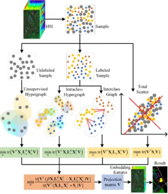
Fig. 2. Procedure of the proposed SSDHL method.
function can be represented as the following:
min Y 1 2 ei∈EH wei dei (xj,xk)∈ei √yj dvj − yk √ dvk 2=tr(YLHYT) s.t. tr(n1YYT) = 1 (5) where LH=I−(Dv)−1/2HWH(De)−1(H)T(Dv)−1/2 is
the hyper-Laplacian matrix.WH = diag([we
1, w2e, . . . , wen])is the weight matrix. De= diag([de
1, de2, . . . , den]) and Dv =
diag([dv
1, dv2, . . . , dvn])are the diagonal matrices of the vertex and hyperedge degrees.
III. SEMISUPERVISEDDISCRIMINANTHYPERGRAPH LEARNING(SSDHL)
In this section, we propose a semisupervised hypergraph learning model to extract the low-dimensional features of an HSI with both the labeled and unlabeled samples. This model is termed as SSDHL. First, an unsupervised hypergraph is con-structed to reveal the similarity of the unlabeled samples, and an intraclass hypergraph is designed to represent the relationships of the labeled samples from the same class. To enhance the discriminant performance of different classes, we also construct an interclass graph to separate the samples from different classes as much as possible. In addition, a total scatter matrix is used to disperse the distribution of all the labeled and unlabeled samples. A semisupervised DR model is constructed to compact the similar properties of the unsupervised hypergraph and the intraclass hypergraph and separate the difference characteristics of the interclass graph and the total scatter matrix. The workflow of the proposed SSDHL method is shown in Fig. 2.
A. Unsupervised Hypergraph
For the unlabeled samples, an unsupervised hypergraph
GH
u ={Xu,EHu,WHu}is constructed to represent the multiple relationships of the unlabeled samples, whereXuis the vertex set of the unlabeled samples,EH
u is the unsupervised hyperedge set, andWH
u is the unsupervised weight matrix of unsupervised hyperedges.KuNNs are selected by the Euclidean distance to construct an unsupervised incidence matrixHu= [hu
ij]i,j huij =
1, ifxu,j∈ NKu(xu,i)
0, otherwise (6)
whereNKu(xu,i)denotes theKuNNs ofxu,iin the unlabeled set. An unsupervised hyeredgeeu
i ∈EHu possessesKuvertices that areKuNNs ofxu,ifrom the unlabeled samples.
For an unsupervised hyperedge eu
i, the weight is used to represent the similarity of these vertices on this hyperedge as defined in the following:
wiu= xu,j∈NKu(xu,i) exp −||xu,j−xu,i||2 2(tu i)2 (7) wheretui = (1/Ku)
xu,j∈NKu(xu,i)||xu,j−xu,i||is the ker-nel parameter, andWH
u = diag([wu1, w2u, . . . , wnuu])is the un-supervised hyperedge weight matrix.
According to the unsupervised incidence matrix and the unsu-pervised weight matrix, the degrees of vertexxu,iand hyperedge eui are defined to reveal the intrinsic properties of unlabeled samples as the following:
duv,i= nu j=1 wujhuij (8) due,j = nu i=1 huij. (9)
In a low-dimensional space, we should preserve the structures of the unsupervised hypergraph and compact the similar samples as much as possible. Therefore, the objective function can be defined as follows: min V 1 2 eui∈EHu wu i du e,i (xu,j,xu,k)∈eui V Tx u,j du v,j −VTxu,k du v,k 2 . (10) With some mathematical operations, we can simplify the objection function (10) with the following procedure in (11) shown at the bottom of this page, where LH
u =I−
(Du
v)−1/2HuWHu(Due)−1(Hu)T(Duv)−1/2is the unsupervised hyper-Laplacian matrix, andDu
e = diag([due,1, due,2, . . . , due,nu]) 1 2 eui∈EHu wui du e,i (xu,j,xu,k)∈eui V Tx u,j du v,j −VTxu,k du v,k 2 = eui∈EHu wu i du e,i (xu,j,xu,k)∈eui tr ⎛ ⎝VTxu,jxTu,jV du v,j −V Tx u,jxTu,kV duv,jdu v,k ⎞ ⎠ = eui∈EHu wu i du e,i xu,j,xu,k∈Xu huijhuiktr ⎛ ⎝VTxu,jxTu,jV du v,j −V Tx u,jxTu,kV du v,jduv,k ⎞ ⎠ = eui∈EHu xu,j,xu,k∈Xu ⎛ ⎝huik du e,i ×w u ihuijtr(VTxu,jxTu,jV) du v,j −tr(V Txu,jhu ijwuihuikxTu,kV) du e,i duv,jduv,k ⎞ ⎠ = xu,j∈Xu ⎛ ⎜ ⎝tr(VTxu,jxTu,jV) 1 du v,j eui∈EHu ⎛ ⎜ ⎝wiuhuij xu,k∈Xu hu ik du e,i ⎞ ⎟ ⎠ ⎞ ⎟ ⎠ − eui∈EHu xu,j,xu,k∈Xu tr ⎛ ⎝VTx u,j 1 du v,j huijwiu 1 du e,i huik 1 du v,k xT u,kV ⎞ ⎠ = tr(VTXuXTuV) −tr VTX u(Duv)−1 /2HuWH u(Due)−1(Hu) T (Duv)−1/2XTuV = tr VTX u I−(Duv)−1/2HuWHu(Due)−1(Hu)T(Duv)−1/2 XT uV = trVTXuLHuXTuV . (11)
andDu
v = diag([duv,1, duv,2, . . . , duv,nu])are the degree matrices of the unsupervised hyperedges and the vertices.
According to the transformation procedure of (17), for the unlabeled samples, the low-dimension embedding function can be denoted by min V tr VTX uLHuXTuV . (12) B. Intraclass Hypergraph
To reveal the multiple properties of the samples from the same class, we construct an intraclass hypergraph GHw =
{Xl,EH
w,WHw}, where Xl is the vertex set of the labeled samples, EH
w is the intraclass hyperedge set, andWHw is the intraclass weight matrix of intraclass hyperedges. An intraclass incidence matrix can be defined asHw= [hw
ij]i,jvia selecting KwNNs from the same class with the Euclidean distance in the labeled set
hwij =
1, ifxl,j ∈ NKw(xl,i)and(xl,i) =(xl,j)
0, otherwise (13)
where NKw(xl,i)denotes theKw NNs ofxl,i from the same class.
For an intraclass hyperedgeew
i, the hyperedge weight, which reflects the similarity of the vertices on the hyperedgeew
i, is set as the following: wwi = xl,j∈NKw(xl,i) exp −||xl,j−xl,i||2 2(tw i )2 (14) wheretw i = (1/Kw)
xl,j∈NKw(xl,i)||xl,j−xl,i||is the kernel parameter, and WwH= diag([w1w, ww2, . . . , wwnl]) is the intra-class hyperedge weight matrix.
According to the intraclass incidence matrix, we can obtain the degrees of intraclass hyperedgeewi and vertexxl,ito repre-sent the intrinsic properties of hypergraph, i.e.,
dwv,i= nl j=1 wwjhwij (15) dwe,j = nl i=1 hwij. (16)
In a low-dimensional space, the intraclass hypergraph struc-ture is preserved to reveal the intrinsic properties of the labeled samples and the intraclass similar samples are compacted as much as possible. With the derivedhw
ij,dwv,i,wiw, anddwe,j, we can obtain hwr
ij ,dwrv,i, wiwr, and dwre,j of the rth class, and the low-dimensional projection function can be determined by
min V 1 2 c r=1 ewri ∈EH w wwr i dwr e,i (xr,j,xr,k)∈ewri V Tx r,j dwr v,j −VTxr,k dwr v,k 2 (17) where ewr
i is theith hyperedge in therth class,xr,j is thejth sample in therth class,dwr
e,iis the degree of intraclass hyperedge ewr
i , anddwrv,jis the degree of vertexxr,j.
With the same transformation procedure of (11), the low-dimensional embedding function of (17) can be simplified as
min V c r=1 trVTXrLHwrXTrV = min V tr VTX lLHwXTl V (18) where Xr= [xr,j]j is the rth class samples, Xl= [Xr]cr=1,
LH
wr =I−(Dwrv )−1/2HwrWwrH(Dwre )−1(Hwr)T(Dwrv )−1/2 is the intraclass hyper-Laplacian matrix of the rth class, Dwr
e = diag([dwre,1, de,wr2, . . . , dwre,nr]) and D wr v =
diag([dwr
v,1, dwrv,2, . . . , dwrv,nr]) are the degree matrices of the intraclass hyperedges and the vertices of the rth class,
Hwr = [hwr ij ]
nr
i,j=1 is the incidence matrix of the rth class,
nris the number of therth class, andLH
w = diag([LHwr]cr=1)is
the intraclass hyper-Laplacian matrix.
C. Interclass Graph
To further enhance the difference of the samples from different classes, we construct a graph Gb={Xl,Eb,Wb} to reveal the relationships of interclass samples that should be restrained in low-dimensional space. In a graphGb,Xlis the vertex set consisting of the labeled samples,Ebdenotes the interclass edge set, and Wb is the interclass weight matrix of the interclass edges. To construct the graph Gb, we adopt the Euclidean distance to selectKbinterclass NNs and connect each neighbor with an edge. For each edge, we set a weightwb
ij to reveal the similarity of verticesiandj. If two vertices are unconnected, the weight is set to zero. Therefore, the weight can be defined as follows: wbij= ⎧ ⎪ ⎨ ⎪ ⎩ exp(−||xl,j−xl,i||2 2(tbi)2 ), ifxl,j∈NKb(xl,i) and(xl,i)=(xl,j) 0,otherwise (19) wheretb i = (1/Kb)
xl,j∈NKb(xl,i)||xl,j−xl,i||is the kernel parameter.NKb(xl,i)denotes theKbNNs ofxl,ifrom different classes.Wb= [wijb]
nl
i,j=1is the interclass weight matrix. Since
the graph is undirected, the weight matrix should be symmetric and it should be symmetrized toWb= max(Wb,WbT).
The degree of vertexxl,iis denoted as dbv,i=
nl
j=1
wbi,j. (20)
In a low-dimensional space, the relationships ofGbshould be separated as much as possible to restrain the similarity of the interclass NNs. According towb
ijanddbv,i, we can obtaind bp v,iof thepth class andwbpqi between thepth class and theqth class, and an objective function can be defined as follows:
max V 1 2 c p=1 c q=1,q=p np i=1 nq j=1 wbpqij V Tx p,i dbpv,i −VTxq,j dbqv,j 2 (21)
wherexp,i is theith sample from thepth class anddbpv,iis the degree of vertexxp,i.
For (21), we can transform it into another form with the total labeled samples by max V 1 2 nl i=1 nl j=1 wbij V Tx l,i db v,i −VTxl,j db v,j 2 . (22)
With some mathematical operations, (22) can be transformed as a matrix operation as follows:
1 2 nl i=1 nl j=1 wijb V Tx l,i db v,i −VTxl,j db v,j 2 = nl i=1 nl j=1 tr ⎛ ⎝VTx l,i wijb db v,i xT l,iV−VTxl,i wijb db v,idbv,j xT l,jV ⎞ ⎠ = tr ⎛ ⎝VT ⎧ ⎨ ⎩ nl i=1 xl,i nl j=1wijb db v,i xT l,i − nl i,j=1 ⎛ ⎝xl,i wbij db v,idbv,j xT l,i ⎞ ⎠ ⎫ ⎬ ⎭V ⎞ ⎠ = tr VT n l i=1 (xl,ixTl,i) − nl i,j=1 xl,i(dbv,i) −1/2 wijb(dbv,j) −1/2 xT l,i ⎤ ⎦V ⎞ ⎠ = tr(VTXl[I−(Dbv) −1/2 Wb(Dbv) −1/2 ]XTlV) = tr(VTXlLbXTlV) (23) whereLb=I−(Dbv) −1/2W b(Dbv) −1/2
denotes the interclass Laplacian matrix, andDb
v = diag(dbv,1, dbv,2, . . . , dbv,nl)is the diagonal matrix of the vertex degree.
According to (23), the interclass graph embedding function can be simplified as max V tr VTX lLbXTlV . (24) D. Total Scatter
To better combine the labeled and unlabeled samples, we construct a total scatter matrix to control the distribution of all the samples. The total scatter matrix is defined as the following:
St= n i=1 (xi−X¯)(xi−X¯) T (25) whereX¯ = n1ni=1xiis the mean ofX.
In the low-dimensional space, the total scatter should be dis-persed as much as possible to better discriminate these samples from different classes. Therefore, the objective function can be defined as follows: max V tr(V TS tV). (26) E. Feature Embedding
To reduce the heterogeneity of samples from the same class and enhance the difference of samples from different classes, the intraclass samples should be compacted and the interclass samples should be separated as much as possible in the low-dimensional space. According to the intraclass hypergraph, the interclass graph, the unsupervised hypergraph, and the total scatter matrix, we design a combined projection function to obtain the low-dimensional discriminant features and reveal the complex intrinsic properties of an HSI. The projection matrix can be computed by the following optimization problem:
min V tr[VT(βX lLHwXTl +XuLHuXTu)V] tr[VT(X lLbXTl +St)V] = min V tr(VTPlV) tr(VTPgV) (27) whereβ >1is a label weight parameter to enhance the contri-bution of the labeled samples.Pl=βX
lLHwXTl +XuLHuXTu is the local related matrix andPg=X
lLbXTl +Stdenotes the global related matrix. The local related matrix reveals the homo-geneity of the similar samples that may be from the same class, whereas the global related matrix represents the heterogeneity of the differential samples that may be from different classes.
According to the principle of the generalized Rayleigh quo-tient, the optimization function of (27) is equal to the following problem:
min
V V
TPlV
s.t.VTPgV=I. (28) To solve the optimization problem (28), we use the method of Lagrangian multipliers [44], [45] to obtain the optimal pro-jection matrix, and the Lagrangian function can be defined as follows:
L(V,λ) =VTPlV−λ(VTPgV−I) (29) whereλis the Lagrangian multiplier.
To obtain the optimal projection, we set the derivative of L(V,λ) to zero, and the optimization problem can be trans-formed to a generalized eigenvalue problem
Plv
i=λiPgvi (30) whereλiis an eigenvalue and its corresponding eigenvector isvi. The optimization solution is composed of thedlargest eigenval-ues corresponding eigenvectors, and the projection matrix can be denoted as the following:
V= [v1,v2, . . . ,vd]∈ B×d. (31) According to the projection matrix, we can derive the low-dimensional embedding features ofxias
yi=VTxi. (32)
F. Illustration of SSDHL
In summary, the proposed SSDHL method constructs an intraclass hypergraph and an interclass graph with the labeled samples to represent the intrinsic properties of the data. SS-DHL also generates an unsupervised hypergraph to reveal the
Fig. 3. Botswana HSI. (a) False-color image. (b) Ground truth. (Note that the number of samples for each class is shown in brackets.)
similarity of the unlabeled samples. In addition, a total scatter matrix is designed to control the distribution of all the samples, which can better combine the labeled and unlabeled samples. For SSDHL, the local information is represented with the intraclass and unsupervised hypergraphs, whereas the global information is described with the interclass graph and the total scatter matrix. The proposed method can use a few labeled samples and a large number of unlabeled samples to effectively reveal the intrinsic structures of the HSI data, and it can better extract the low-dimensional embedding features to improve the discriminant performance of an HSI. The detailed procedure of SSDHL is shown in Algorithm 1.
IV. EXPERIMENTALRESULTS
To demonstrate the effectiveness of the proposed SSDHL, we conduct comprehensive experiments on three publicly available HSI data sets and benchmarked with a few state-of-the-art methods for comparison and performance evaluation.
A. Data Sets
1) Botswana Data Set: This data set was captured by the NASA Earth Observing-1 satellite over the Okavango Delta, Botswana on May 31, 2001. The spatial resolution is 30 m with a size of 1476×256 pixels. This image contains 242 bands with the electromagnetic spectrums in the range of 400–2500 nm. Af-ter removing noise and waAf-ter absorption bands, the retained 145 bands were used for scientific research. This data set contains 3428 labeled samples in 14 types of land cover. The false-colored image and the ground truth are shown in Fig. 3.
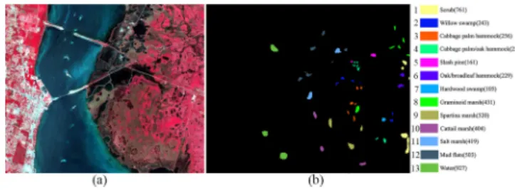
2) KSC Data Set:This data set was acquired by the NASA Airborne Visible Infrared Imaging Spectrometer sensor over the Kennedy Space Center (KSC) on March 23, 1996. The image has a spatial resolution of 18 m with 224 electromagnetic spectrum bands. Due to the influence of water absorption and low signal-to-noise ratio, only 176 bands were retained for experimental analysis. This data set has a size of 512×614 pixels and a total of 5211 pixels were labeled in 13 types of land cover. Fig. 4 displays the false color image and its corresponding ground truth.
3) PaviaU Data Set:This image was captured by the Reflec-tive Optics System Imaging Spectrometer sensor in 2001. The
Fig. 4. KSC HSI. (a) False-color image. (b) Ground truth. (Note that the number of samples for each class is shown in brackets.)
Algorithm 1:SSDHL.
Input:Labeled samples
Xl= [xl,1,xl,2, . . . ,xl,nl]∈RB×nland their corresponding class labels
{(xl,1), (xl,2), . . . , (xl,nl)} ∈ {1,2, . . . , c}, unlabeled samplesXu= [xu,1,xu,2, . . . ,xu,nu]∈RB×nu,
X= [Xl,Xu]∈RB×n, embedding dimensiond(d<B), neighbor sizeKu,Kw,Kb, and weight parameterβ >1.
Output:Low-dimensional embedding features
Y= [y1,y2, . . . ,yn]∈ d×n.
1: Construct the intraclass hypergraphGHw with theKw nearest neighbors from the same class according to Euclidean distances in the labeled samples.
2: Compute the intraclass hyper-Laplacian matrix of the
rth class:
3: LH
wr =I−(Dwrv )−1/2HwrWHwr(Dwre )−1
(Hwr)T(Dwr v )−1/2
4: Achieve the intraclass hyper-Laplacian matrix:
5: LH
w = diag([LHwr]cr=1)
6: Construct the unsupervised hypergraphGH
u with the Kunearest neighbors according to Euclidean distances in the unlabeled samples.
7: Compute the unsupervised hyper-Laplacian matrix: 8: LHu =I−(Duv)−1/2HuWHu(Due)−1
(Hu)T(Duv)−1/2
9: Construct the interclass graphGbwith theKbnearest neighbors from different classes according to
Euclidean distances in the labeled samples. 10: Lb=I−(Dbv)
−1/2
Wb(Dbv) −1/2
11: Construct the total scatter matrix with all the samples as:
12: St=
n
i=1(xi−X¯)(xi−X¯) T 13: Compute the local related matrix: 14: Pl=βX
lLHwXTl +XuLHuXTu 15: Compute the global related matrix:
16: Pg=X
lLbXTl +St
17: Solve the generalized eigenvalue problem: 18: Plv
i=λiPgvi
19: Obtain the projection matrix withdlargest eigenvalues corresponding eigenvectors:
20: V= [v1,v2, . . . ,vd]∈ B×d
21: Calculate the low-dimensional embedding features: 22: yi=VTxi
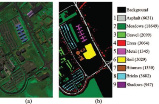
Fig. 5. PaviaU HSI. (a) False color image. (b) Ground truth. (Note that the number of samples for each class is shown in brackets.)
image scene covers the University of Pavia (PaviaU) with a size of 610×340 pixels. Since 12 bands are influenced by noise and water absorption, the remaining 103 bands are used for scientific research. This data set has 9 land cover types and 42776 labeled samples. The false color image and its ground truth are shown in Fig. 5.
B. Experimental Setup
In the experiments, we randomly selected a few samples from a data set as the labeled set and a large number of samples from the remaining samples as the unlabeled set. The training set consists of the labeled and unlabeled sets, and the other samples are composed of the test set. First, we use the training set to train each DR model, where the unsupervised and semisupervised methods use all the labeled and unlabeled samples for training and the supervised methods just use the labeled samples for training. Then, we can obtain the low-dimensional embedding features of all the samples with these DR models. Finally, a classifier is used to discriminate the class type of each test sample; meanwhile, we apply the classification accuracy of each class, the average accuracy of all the classes (AA), the overall classification accuracy (OA), and the kappa coefficient (KC) to quantitatively evaluate the classification results of each method. As we proposed a semisupervised DR method in this article, some similar DR methods are used for comparison. To demon-strate the efficacy of the proposed method, we selected several semisupervised methods for comparison, i.e., SDA, SSMMC, S3MPE, and S3MDA. In addition, we compared two hypergraph learning methods, termed BH and DHLP. After extracting the embedding features, three nonparameter classifiers were used for classification, including the NN classifier, the spectral angle mapping (SAM) classifier, and the sparse representation clas-sifier (SRC) [46]. Meanwhile, we also took the classification results of the raw spectral feature with NN, SAM, and SRC as the baseline (BL) for comparison.
In the experiments, to compare the classification result of each method, we randomly selected 20 labeled samples from each class and 1000 unlabeled samples from the remaining samples to form the training set. All other samples were used as the test set. For the neighbor sizeKw,Ku, andKb, for convenience, we setKu=KwandKb=αKw. This is becauseKwandKuare both used to reveal the similar relationship of the homogeneous samples, whereas Kb is used to represent the heterogeneous
structure of the interclass samples; generally,Kbis larger than Kw. Therefore, for the neighbor size, we just need to set the values ofKwandαin the experiments, andKwandαare set to 7 and 5 for the Botswana data set, 9 and 9 for the KSC data set, and 9 and 5 for the PaviaU data set. For the weight parameterβ, we set it to 3 for the Botswana data set and 5 for the KSC and PaviaU data sets. For all the methods, the embedding dimension is set to 30. To robustly analyze each algorithm, we repeated each experiment ten times in each condition and obtained the average OAs with standard deviations (STDs) and the average KCs. All the experiments were conducted on a personal computer with E5-2620 v3 central processing unit, 16-GB memory, and 64-b Windows 10 using MATLAB 2017b.
C. Performance Comparison
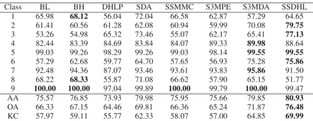
To compare the classification results of each method, we used the training set containing 20 labeled samples from each class and 1000 unlabeled samples to learn the projection model of each method. For the supervised methods, only the labeled samples were used for training. According to the training models, we can obtain the low-dimensional features of each method. Then, we adopted the NN classifier to discriminate the labels of the test set. The classification results on the three data sets are shown in Tables I –III, where the bold font denotes the best result in each row.
According to Tables I–III, the proposed method obtains better results than the other semisupervised methods (i.e., SDA, SS-MMC, S3MPE, and S3MDA) in most classes and generates the best AA, OA, and KC, which indicates that the proposed method can more effectively reveal the complex intrinsic properties of the HSI and enhance the compactness of the homogeneous samples and the separability of the heterogeneous samples. Compared with two hypergraph learning methods (i.e., BH and DHLP), the proposed SSDHL method achieves better classifi-cation results, because SSDHL can simultaneously utilize the labeled and unlabeled samples to train the projection model, whereas DHLP just uses the labeled samples and BH does not apply the label information, which, both, cannot obtain good discriminant features to improve the classification performance of an HSI.
To visualize the classification results, Figs. 6 –8 display the classification maps of the Botswana, KSC, and PaviaU data sets. In the figures, SSDHL achieves more homogeneous areas than the other methods on three data sets, especially in the regions of
Water,Hippo Grass,Floodplain Grasses 1,Floodplain Grasses 2,Reeds 1,Riparian,Island Interior,Acacia Woodlands, Aca-cia Shrublands, andShort Mopanefor the Botswana data set,
Cabbage Palm Hammock,Slash Pine,Oak/Broadleaf Hammock,
Graminoid Marsh, andSalt Marsh for the KSC data set, and
MeadowsandGravelfor the PaviaU data set. The reason is that SSDHL constructs an intraclass hypergraph and an interclass graph to enhance the discrimination of labeled samples and a total scatter matrix to maximize the variance distribution of the labeled and unlabeled samples. The results indicate that the pro-posed SSDHL method can learn a good semisupervised model with the labeled and unlabeled samples to reveal the intrinsic
TABLE I
CLASSIFICATIONRESULTS OFEACHCLASS ON THEBOTSWANADATASET
TABLE II
CLASSIFICATIONRESULTS OFEACHCLASS ON THEKSC DATASET
TABLE III
CLASSIFICATIONRESULTS OFEACHCLASS ON THEPAVIAU DATASET
multiple properties of an HSI and improve the discriminant power of low-dimensional features.
D. Labeled Samples Analysis
To analyze the classification accuracies with respect to dif-ferent numbers of labeled samples, we selected 5–40 (with
an interval of 5) labeled samples from each class and 1000 unlabeled samples from the remaining samples of each data set, and the other samples were used for testing. After obtaining the embedding features, we adopt the NN classifier to discriminate the labels of the test samples. Fig. 9 shows the classification results with different numbers of labeled samples on the three data sets.
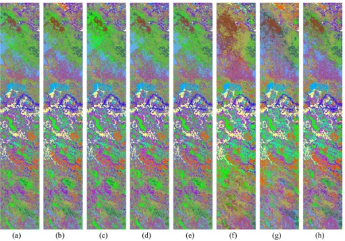
Fig. 6. Classification maps of each method on the Botswana data set. (a) BL. (b) BH. (c) DHLP. (d) SDA. (e) SSMMC. (f) S3MPE. (g) S3MDA. (h) SSDHL.
Fig. 7. Classification maps of each method on the KSC data set. (a) BL. (b) BH. (c) DHLP. (d) SDA. (e) SSMMC. (f) S3MPE. (g) S3MDA. (h) SSDHL.
According to Fig. 9, we can obtain the same conclusion about the change in the number of labeled samples on the three data sets. With the increase in the number of labeled samples, the classification results first increase and then reach to a peak value. The reason is that the more priori information can be used to im-prove the classification accuracies with the increased number of labeled samples. When the number of labeled samples exceeds a certain value, there is adequate information to represent the intrinsic properties of an HSI, which will make the classification accuracy maintain a stable value, hence no further improvement from increasing the number of labeled samples.
E. Unlabeled Samples Analysis
To analyze the classification results with different numbers of unlabeled samples, we fixed the number of labeled samples to 20 in each class, and we set the number of unlabeled samples
to{50,100,300,500,1000,1500,and2000}. The classification results with the NN classifier with different numbers of unla-beled samples are shown in Fig. 10.
As shown in Fig. 10, with the increasing number of unla-beled samples, the OAs and KCs improve and then reach to a stable value, because a large number of unlabeled samples can reduce the influence of outlier samples and provide more available information. The results indicate that the unlabeled samples are beneficial to promote the extraction of the intrinsic structures of the HSI and enhance the representation power of the embedding features.
F. Dimensionality Analysis
For DR, the embedding dimension will influence the classifi-cation result. Thus, we conduct further experiments to analyze the OAs with respect to the embedding dimension. The results
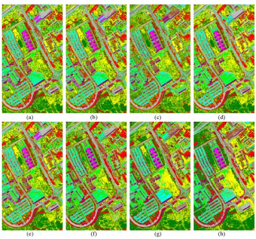
Fig. 8. Classification maps of each method on the PaviaU data sets. (a) BL. (b) BH. (c) DHLP. (d) SDA. (e) SSMMC. (f) S3MPE. (g) S3MDA. (h) SSDHL.
Fig. 9. Classification results with different numbers of labeled samples on (a) Botswana, (b) KSC, and (c) PaviaU data sets.
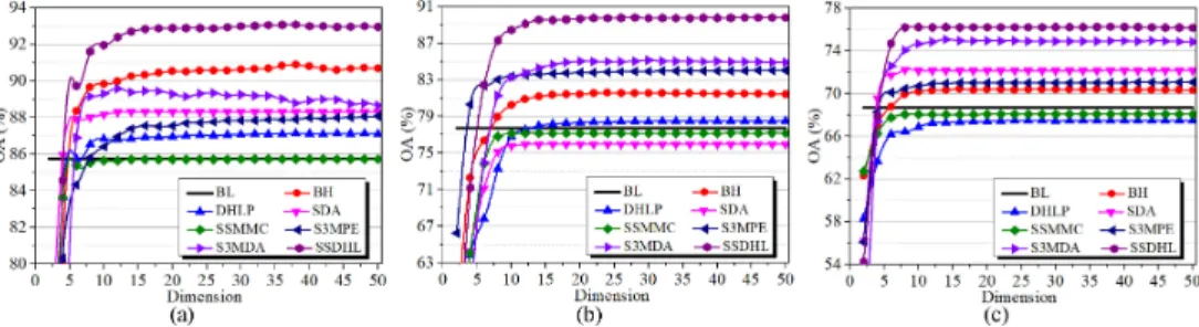
Fig. 11. Classification results with different embedding dimensions on (a) Botswana, (b) KSC, and (c) PaviaU data sets.
TABLE IV
CLASSIFICATIONRESULTSWITHDIFFERENTCLASSIFIERS ON THEBOTSWANADATASET
TABLE V
CLASSIFICATIONRESULTSWITHDIFFERENTCLASSIFIERS ON THEKSC DATASET
with the NN classifier under different embedding dimensions are shown in Fig. 11.
In Fig. 11, the OAs improve with the increase in the embed-ding dimension and then reach a peak value for each method, be-cause a large embedding dimension contains more information to enhance the discriminant power of low-dimensional features. Most methods generate better OAs than BL on the three data sets, which indicates that the classification results will improve after using the process of DR. This is because these DR methods reduce the redundant information and enhance the discriminat-ing power of features. The proposed method achieves the best classification accuracies than the other methods under different embedding dimensions on the Botswana, KSC, and PaviaU data sets. The reason is that the proposed method can reveal the multiple structures of an HSI and enhance the compactness of the intraclass samples and the separability of the interclass samples. To obtain better classification accuracy, we set the embedding dimension to 30 for all the methods on the three data sets.
G. Results on Different Classifiers
To demonstrate the effectiveness of the proposed method for different classifiers, we selected NN, SAM, and SRC to discriminate the labels of test samples after extracting the
low-dimensional features. In this experiments, again 20 labeled samples from each class and 1000 unlabeled samples were used to train the DR models and the classification results with the three classifiers are given in Tables IV–VI.
According to Tables IV–VI, SSDHL achieves the best clas-sification accuracies in terms of OA and KC than the other methods on the three data sets, because the proposed method considers the multiple structures to represent the homogenous properties of an HSI, the binary relationships to reveal the heterogeneous information of the HSI, and the total scatter to control the distribution of the labeled and unlabeled samples in the HSI. SSDHL can compact the homogenous samples and separate the heterogeneous samples to improve the discriminant performance of low-dimensional features with the labeled and unlabeled samples.
H. Parameter Analysis
In the proposed method, it has two neighbor size parameters Kwandα, and a label weight parameterβ. Thus, we conduct two experiments to analyze the neighbor size and the label weight for the influence of classification accuracy.
1) Neighbor Size: For the neighbor size parametersKwand α, we randomly selected 20 labeled samples from each class
TABLE VI
CLASSIFICATIONRESULTSWITHDIFFERENTCLASSIFIERS ON THEPAVIAU DATASET
Fig. 12. Classification results with respect to the intraclass neighborKwand the interclass neighborKb=αKwon (a) Botswana, (b) KSC, and (c) PaviaU data sets.
Fig. 13. Classification results with respect to the label weightβon (a) Botswana, (b) KSC, and (c) PaviaU data sets. and 1000 unlabeled samples to conduct this experiment, and
then we used the NN classifier to discriminate the labels of the other samples. Fig. 12 shows the average classification results about the change ofKwandαwith ten repeated experiments.
According to Fig. 12, the classification accuracy is fluctuating under differentKwandαon the three data sets, and the fluctu-ation is very small in an appropriate range. For the Botswana data set, the results with smallKwandαare better than those with large values, whereKwandαare set to 7 and 5. For the KSC data set, the parametersKwandαhave a small influence in terms of the classification accuracy, and we set them to 9 and 9. For the PaviaU data set, the OAs improve with the increase inKwandαand then decrease whenKwandαexceed a value, thus we setKwandαto 9 and 5.
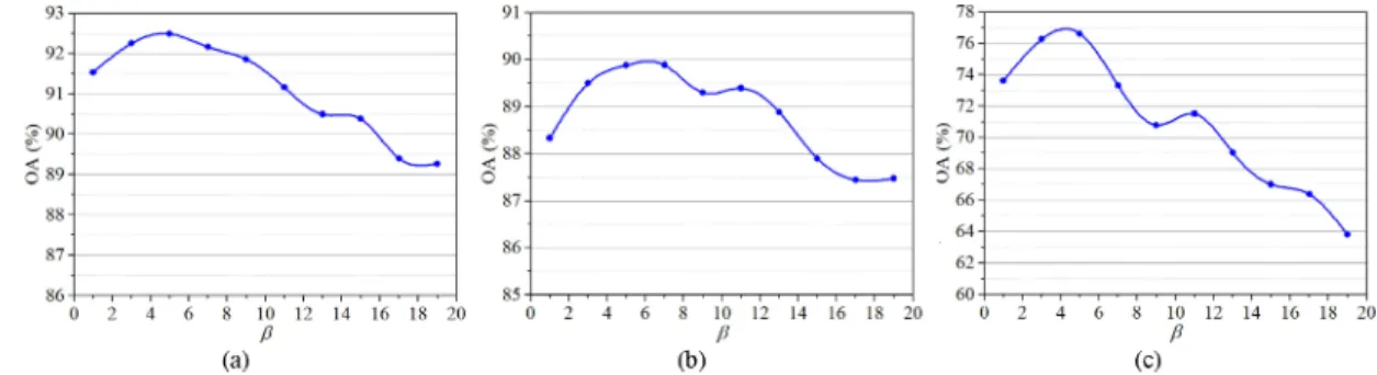
2) Label Weight: To enhance the contribution of the labeled samples, we analyzed the classification accuracy with respect to the label weightβand used the training set including 20 labeled samples from each class and 1000 unlabeled samples. Fig. 13
displays the classification results with differentβ on the three data sets.
In Fig. 13, the OAs first increase and then decrease with the increase inβ. The reason is that a large weight will enhance the contribution of the labeled samples to better represent the intrinsic properties of the HSI. Whenβ exceeds a certain value and continues to increase, it will degrade the contribution of the unlabeled samples, which cannot effectively reflect the distribu-tion of the HSI. Therefore, we setβto 5 for the Botswana, KSC, and PaviaU data sets.
V. CONCLUSION ANDDISCUSSION
In this article, we proposed an SSDHL method for DR in an HSI. In SSDHL, we utilize the labeled samples to construct an intraclass hypergraph and an interclass graph; meanwhile, we use the unlabeled samples to design an unsupervised hypergraph. In addition, a total scatter matrix is adopted to control the
distribution of the labeled and unlabeled samples. Then, we construct an objective function to obtain the projection matrix, which can compact the intraclass hypergraph and the unsuper-vised hypergraph and separate the interclass graph and the total scatter matrix as much as possible. Finally, we use three data sets (Botswana, KSC, and PaviaU) to demonstrate the effectiveness of the proposed method. The proposed method achieves better classification accuracy compared with a few state-of-the-art algorithms. SSDHL can compact the homogenous information in the intraclass hypergraph and the unsupervised hypergraph to represent the intrinsic properties of the samples from the same class while it can also separate the heterogeneous information in the interclass graph and the total scatter matrix to enhance the discriminant performance of the samples from different classes. In the classification maps, there still exist salt and pepper noise in the homogeneous areas for these methods does not consider the spatial relationship of HSIs. However, the spatial distribution is very important in HSI. Therefore, we can apply the spatial information to develop spatial-spectral semisupervised method in the future.
In addition, the proposed method needs to set two important neighbor parameters, which is very difficult to select a proper value; because the neighbor structures may be different for each class land cover in an HSI. If using the stable neighbor sizes to represent different land-cover types, we may not achieve satisfactory classification results for an HSI. Thus, in the future, self-adaption semisupervised learning can be designed based on SSDHL to represent the intrinsic information of an HSI.
ACKNOWLEDGMENT
The authors would like to thank the handling editor and the anonymous reviewers for their detailed and constructive comments and suggestions, which indeed helped to improve the quality of this article.
REFERENCES
[1] W. Sun, G. Yang, J. Peng, and Q. Du, “Hyperspectral band selection using weighted kernel regularization,”IEEE J. Sel. Topics Appl. Earth Observ. Remote Sens., vol. 12, no. 9, pp. 3665–3676, Sep. 2019.
[2] L. Zhang, L. Zhang, B. Du, J. You, and D. Tao, “Hyperspectral image unsupervised classification by robust manifold matrix factorization,”Inf. Sci., vol. 485, pp. 154–169, Feb. 2019.
[3] J. Peng and Q. Du, “Robust joint sparse representation based on maximum correntropy criterion for hyperspectral image classification,”IEEE Trans. Geosci. Remote Sens., vol. 55, no. 12, pp. 7152–7164, Dec. 2017. [4] J. Zabalzaet al., “Novel two-dimensional singular spectrum analysis for
effective feature extraction and data classification in hyperspectral imag-ing,”IEEE Trans. Geosci. Remote Sens., vol. 53, no. 8, pp. 4418–4433, Aug. 2015.
[5] W. Sun, J. Peng, G. Yang, and Q. Du, “Correntropy-based sparse spectral clustering for hyperspectral band selection,”IEEE Geosci. Remote Sens. Lett., vol. 17, no. 3, pp. 484–488, Mar. 2020.
[6] Z. Lv, T. Liu, P. Zhang, J. Benediktsson, T. Lei, and X. Zhang, “Novel adap-tive histogram trend similarity approach for land cover change detection by using bitemporal very-high-resolution remote sensing images,”IEEE Trans. Geosci. Remote Sens., vol. 57, no. 12, pp. 9554–9574, Dec. 2019. [7] X. Zheng, Y. Yuan, and X. Lu, “Dimensionality reduction by
spatial-spectral preservation in selected bands,” IEEE Trans. Geosci. Remote Sens., vol. 55, no. 9, pp. 5185–5197, Sep. 2017.
[8] G. Jin et al., “An advanced phase synchronization scheme for LT-1,” IEEE Trans. Geosci. Remote Sens., vol. 58, no. 3, pp. 1735–1746, Mar. 2020.
[9] W. Sun and Q. Du, “Hyperspectral band selection: A review,”IEEE Geosci. Remote Sens. Mag., vol. 7, no. 2, pp. 118–139, Jun. 2019.
[10] F. Luo, L. Zhang, B. Du, and L. Zhang, “Dimensionality reduction with en-hanced hybrid-graph discriminant learning for hyperspectral image classi-fication,”IEEE Trans. Geosci. Remote Sens., vol. 58, no. 8, pp. 5336–5353, Aug. 2020.
[11] J. Zabalzaet al., “Novel folded-PCA for improved feature extraction and data reduction with hyperspectral imaging and SAR in remote sensing,” ISPRS J. Photogramm. Remote Sens., vol. 93, pp. 112–122, 2014. [12] W. Sun, G. Yang, J. Peng, and Q. Du, “Lateral-slice sparse tensor robust
principal component analysis for hyperspectral image classification,”IEEE Geosci. Remote Sens. Lett., vol. 17, no. 1, pp. 107–111, Jan. 2020. [13] H. Wang, X. Lu, Z. Hu, and W. Zheng, “Fisher discriminant analysis with
L1-norm,”IEEE Trans. Cybern., vol. 44, no. 6, pp. 828–842, Jun. 2014. [14] L. Guan, W. Xie, and J. Pei, “Segmented minimum noise fraction
trans-formation for efficient feature extraction of hyperspectral images,”Pattern Recognit., vol. 48, no. 10, pp. 3216–3226, Oct. 2015.
[15] C. M. Bachmann, T. L. Ainsworth, and R. A. Fusina, “Exploiting manifold geometry in hyperspectral imagery,”IEEE Trans. Geosci. Remote Sens., vol. 43, no. 3, pp. 441–454, Mar. 2005.
[16] W. Wu, Y. Zhang, Q. Wang, F. Liu, P. Chen, and H. Yu, “Low-dose spectral CT reconstruction using image gradient0-norm and tensor dictionary,” Appl. Math. Model., vol. 63, pp. 538–557, Jul. 2018.
[17] J. Tenenbaum, V. de Silva, and J. Langford, “A global geometric frame-work for nonlinear dimensionality reduction,”Science, vol. 290, no. 5500, pp. 2319–2323, Dec. 2000.
[18] S. Roweis and L. Saul, “Nonlinear dimensionality reduction by locally linear embedding,”Science, vol. 290, no. 5500, pp. 2323–2326, Dec. 2000. [19] M. Belkin and P. Niyogi, “Laplacian eigenmaps for dimensionality reduction and data representation,” Neural Comput., vol. 15, no. 6, pp. 1373–1396, Jun. 2003.
[20] X. He, D. Cai, S. Yan, and H. Zhang, “Neighborhood preserving embed-ding,” inProc. IEEE Int. Conf. Comput. Vision, Dec. 2005, pp. 1208–1213. [21] R. Wang, F. Nie, R. Hong, X. Chang, X. Yang, and W. Yu, “Fast and orthogonal locality preserving projections for dimensionality reduction,” IEEE Trans. Image Process., vol. 26, no. 10, pp. 5019–5030, Oct. 2017. [22] S. Yan, D. Xu, B. Zhang, H. Zhang, Q. Yang, and S. Lin, “Graph embedding
and extensions: A general framework for dimensionality reduction,”IEEE Trans. Pattern Anal. Mach. Intell., vol. 29, no. 1, pp. 40–51, Jan. 2007. [23] M. Sugiyama, “Dimensionality reduction of multimodal labeled data
by local fisher discriminant analysis,” J. Mach. Learn. Res., vol. 8, pp. 1027–1061, May 2007.
[24] Y. Zhou, J. Peng, and C. L. P. Chen, “Dimension reduction using spatial and spectral regularized local discriminant embedding for hyperspectral image classification,”IEEE Trans. Geosci. Remote Sens., vol. 53, no. 2, pp. 1082–1095, Sep. 2015.
[25] F. Luo, H. Hong, Y. Duan, J. Liu, and Y. Liao, “Local geometric structure feature for dimensionality reduction of hyperspectral imagery,”Remote Sens., vol. 9, no. 8, Aug. 2017, Art. no. 790.
[26] Q. Shi, L. Zhang, and B. Du, “Semisupervised discriminative locally enhanced alignment for hyperspectral image classification,”IEEE Trans. Geosci. Remote Sens., vol. 51, no. 9, pp. 4800–4815, Sep. 2013. [27] K. Tan, J. Hu, J. Li, and P. Du, “A novel semi-supervised hyperspectral
image classification approach based on spatial neighborhood information and classifier combination,”ISPRS J. Photogramm. Remote Sens., vol. 105, pp. 19–29, Jul. 2015.
[28] S. Yang, P. Jin, B. Li, L. Yang, W. Xu, and L. Jiao, “Semisupervised dual-geometric subspace projection for dimensionality reduction of hy-perspectral image data,”IEEE Trans. Geosci. Remote Sens., vol. 52, no. 6, pp. 3587–3593, Jun. 2014.
[29] Y. Song, F. Nie, C. Zhang, and S. Xiang, “A unified framework for semi-supervised dimensionality reduction,”Pattern Recognit., vol. 41, no. 9, pp. 2789–2799, Sep. 2008.
[30] R. Luo, W. Liao, X. Huang, Y. Pi, and W. Philips, “Feature extraction of hyperspectral images with semisupervised graph learning,”IEEE J. Sel. Topics Appl. Earth Observ. Remote Sens., vol. 9, no. 9, pp. 4389–4399, Sep. 2016.
[31] D. Cai, X. He, and J. Han, “Semi-supervised discriminant analysis,” in Proc. IEEE Int. Conf. Comput. Vision, Dec. 2007, pp. 1–7.
[32] W. Liao, A. Pižurica, P. Scheunders, W. Philips, and Y. Pi, “Semisupervised local discriminant analysis for feature extraction in hyperspectral images,” IEEE Trans. Geosci. Remote Sens., vol. 51, no. 1, pp. 184–198, Jan. 2013. [33] Y. Song, F. Nie, and C. Zhang, “Semi-supervised sub-manifold discrim-inant analysis,”Pattern Recognit. Lett., vol. 29, no. 13, pp. 1806–1813, Oct. 2008.
[34] F. Luo, H. Huang, Z. Ma, and J. Liu, “Semisupervised sparse manifold dis-criminative analysis for feature extraction of hyperspectral images,”IEEE Trans. Geosci. Remote Sens., vol. 54, no. 10, pp. 6197–6211, Oct. 2016. [35] D. Zhou, J. Huang, and B. Schölkopf, “Learning with hypergraphs:
Clus-tering, classification, and embedding,” inProc. Neural Inf. Process. Syst., Dec. 2006, vol. 19, pp. 1601–1608.
[36] J. Yu, D. Tao, and M. Wang, “Adaptive hypergraph learning and its application in image classification,”IEEE Trans. Image Process., vol. 21, no. 7, pp. 3262–3272, Jun. 2012.
[37] F. Luo, L. Zhang, X. Zhou, T. Guo, Y. Cheng, and T. Yin, “Sparse-adaptive hypergraph discriminant analysis for hyperspectral image classification,” IEEE Geosci. Remote Sens. Lett., vol. 17, no. 6, pp. 1082–1086, Jun. 2020. [38] S. Gao, I. W. Tsang, and L. Chia, “Laplacian sparse coding, hypergraph Laplacian sparse coding, and applications,”IEEE Trans. Pattern Anal. Mach. Intell., vol. 35, no. 1, pp. 92–104, Jun. 2013.
[39] Z. Zhang, L. Bai, Y. Liang, and E. Hancock, “Joint hypergraph learning and sparse regression for feature selection,”Pattern Recognit., vol. 63, pp. 291–309, Mar. 2017.
[40] H. Yuan and Y. Y. Tang, “Learning with hypergraph for hyperspectral image feature extraction,”IEEE Geosci. Remote Sens. Lett., vol. 12, no. 8, pp. 1695–1699, Aug. 2015.
[41] S. Huang, D. Yang, Y. Ge, and X. Zhang, “Discriminant hyper-Laplacian projections and its scalable extension for dimensionality reduction,” Neu-rocomputing, vol. 173, pp. 145–153, Jan. 2016.
[42] Y. Sun, S. Wang, Q. Liu, R. Hang, and G. Liu, “Hypergraph embedding for spatial-spectral joint feature extraction in hyperspectral images,”Remote Sens., vol. 9, no. 5, May 2017, Art. no. 506.
[43] F. Luo, B. Du, L. Zhang, L. Zhang, and D. Tao, “Feature learning using spatial-spectral hypergraph discriminant analysis for hyperspectral image,”IEEE Trans. Cybern., vol. 49, no. 7, pp. 2406–2419, Jun. 2019. [44] M. Xu, D. Hu, F. Luo, F. Liu, S. Wang, and W. Wu, “Limited angle
X ray CT reconstruction using image gradient0 norm with dictionary learning,”IEEE Trans. Radiat. Plasma Med. Sci., to be published, doi:
10.1109/TRPMS.2020.2991887..
[45] W. Wu, P. Chen, S. Wang, V. Vardhanabhuti, F. Liu, and H. Yu, “Image-domain material decomposition for spectral CT using a generalized dic-tionary learning,”IEEE Trans. Radiat. Plasma Med. Sci., to be published, doi:10.1109/TRPMS.2020.2997880.
[46] J. Wright, A. Y. Yang, A. Ganesh, S. S. Sastry, and Y. Ma, “Robust face recognition via sparse representation,”IEEE Trans. Pattern Anal. Mach. Intell., vol. 31, no. 2, pp. 210–227, Feb. 2009.
Fulin Luo(Member, IEEE) received the B.S. de-gree in mechanical engineering and automation from Southwest Petroleum University, Chengdu, China, in 2011, and the M.S. and Ph.D. degrees in instrument science and technology from Chongqing University, Chongqing, China, in 2013 and 2016, respectively.
He is currently an Associate Researcher with the State Key Laboratory of Information Engineering in Surveying, Mapping and Remote Sensing (LIES-MARS), Wuhan University, Wuhan, China. He was a Postdoctoral Researcher in LIESMARS from 2017 to 2019. His research interests include hyperspectral image classification, image processing, sparse representation, and manifold learning in general.
Tan Guoreceived the B.S. degree from the Henan University of Science and Technology, Luoyang, China, in 2011, and the M.S. and Ph.D. degrees from Chongqing University, Chongqing, China, in 2014 and 2017, respectively.
He is currently a Lecturer with the School of Communication and Information Engineering, Chongqing University of Posts and Telecommuni-cations, Chongqing, China. His current research in-terests include biometrics, pattern recognition, and machine learning.
Zhiping Lin (Senior Member, IEEE) received the B.Eng. degree in control engineering from the South China Institute of Technology, Canton, China, in 1982, and the Ph.D. degree in information engineer-ing from the University of Cambridge, Cambridge, U.K., in 1987.
Since 1999, he has been with Nanyang Techno-logical University, Singapore. His current research interests include multidimensional systems and signal processing, statistical and biomedical signal process-ing, and machine learning.
Dr. Lin was the Editor-in-Chief forMultidimensional SystemsandSignal Processingfrom 2011 to 2015. He was an Associate Editor for the IEEE TRANSACTIONS ONCIRCUITS ANDSYSTEMSII from 2010 to 2011. He was a Reviewer ofMathematical Reviewsfrom 2011 to 2013. He is currently a Subject Editor for theJournal of the Franklin Institute. He was the recipient (as a coauthor) of the 2007 Young Author best paper award from the IEEE Signal Processing Society, the Distinguished Lecturer of the IEEE Circuits and Systems Society from 2007 to 2008, and received the best paper awards from International Conference of Extreme Learning Machine (ELM2015 and ELM2017).
Jinchang Ren (Senior Member, IEEE) received the Ph.D. degree in electronic imaging and media communication from Bradford University, Bradford, U.K., in 2009.
He is currently a Senior Lecturer with the Cen-tre for Excellence for Signal and Image Processing and the Deputy Director of the Strathclyde Hyper-spectral Imaging Centre, University of Strathclyde, Glasgow, U.K. His current research interests include visual computing and multimedia signal processing, especially on semantic content extraction for video analysis and understanding and more recently hyperspectral imaging.
Xiaocheng Zhou, photograph and biography not available at the time of publication.