NBER WORKING PAPER SERIES
PRECAUTIONARY SAVING AND CONSUMPTION FLUCTUATIONS Jonathan A. Parker
Bruce Preston
Working Paper9196
http://www.nber.org/papers/w9196
NATIONAL BUREAU OF ECONOMIC RESEARCH 1050 Massachusetts Avenue
Cambridge, MA 02138 September 2002
For helpful comments, we thank Charles Fleischman, Pierre Olivier Gourinchas, Bo Honore, Andrew Samwick, Chris Sims and seminar participants at the Australian National University, University of Chicago Graduate School of Business, Dartmouth College, Princeton University, the Reserve Bank of Australia, and the 2001 North American Winter Meeting of the Econometric Society. For financial support, Parker thanks the National Science Foundation grant SES-0096076, the Sloan Foundation, and a National Bureau of Economic Research Aging and Health Economics Fellowship through National Institute on Aging grant number T32 AG00186 and Preston thanks the Fellowship of Woodrow Wilson Scholars. The views expressed herein are those of the authors and not necessarily those of the National Bureau of Economic Research.
© 2002 by Jonathan A. Parker and Bruce Preston. All rights reserved. Short sections of text, not to exceed two paragraphs, may be quoted without explicit permission provided that full credit, including © notice, is given to the source.
Precautionary Saving and Consumption Fluctuations Jonathan A. Parker and Bruce Preston
NBER Working Paper No. 9196 September 2002
JEL No. E21, D91
ABSTRACT
This paper uses data on the expenditures of households to explain movements in the average growth rate of consumption in the U.S. from the beginning of 1982 to the end of 1997. We propose and implement a decomposition of consumption growth into series representing four proximate causes. These are new information, and three causes of predictable consumption growth: intertemporal substitution, changes in the preferences for consumption, and incomplete markets for consumption insurance. Incomplete markets for trading consumption in future states leads to statistically significant and countercyclical movements in expected consumption growth. The economic importance of precautionary saving rivals that of the real interest rate, but the relative importance of each source of movement in the volatility of consumption is not precisely measured.
Jonathan Parker Bruce Preston
Department of Economics Department of Economics
416 Robertson Hall 416 Robertson Hall
Princeton University Princeton University
Princeton, NJ 08544 Princeton, NJ 08544
and NBER
1. Introduction
According to canonical macroeconomic theory, aggregate consumption is the result of the optimal choices of a representative consumer. Consumption growth changes over time due to changes in the risk-free rate of return and changes in the information that the consumer has about current wealth, future income, and future rates of return. Con-sistent with this approach, consumption growth is largely unpredictable. But contrary to the canonical theory, predictable movements in aggregate consumption growth have little correlation with the risk-free rate of return and significant correlation with pre-dictable movements in income. For the representative agent approach, there are several puzzling features of US consumption data, such as excess sensitivity, excess smoothness, and the equity premium puzzle.1
This paper measures the relative importance of new information, the real inter-est rate, the preference for consumption, and precautionary saving for movements in average consumption growth. We develop a method that uses the consumption Euler equation and survey data on the consumption expenditures of households to decompose consumption growth into these four proximate causes, and factors outside the model. Using both estimates and calibrations for a standard utility function, we implement this decomposition and find a significant role for precautionary saving in consumption fluctuations.
We focus particularly on predictable movements in consumption growth caused by changes in the amount of consumption risk faced by households, or precautionary sav-ing. We do this for three reasons. First, because consumers face idiosyncratic risk that they do not completely insure, precautionary saving is potentially a significant determinant of consumption dynamics.2 The consumption dynamics of price-taking households in a model economy without complete consumption insurance can be quite 1Flavin (1981), Shiller (1982), Hall (1988), Campbell and Deaton (1989), and Campbell and Mankiw (1989).
2Complete consumption insurance is rejected by Nelson (1994), Cochrane (1991), and Attanasio and Davis (1996).
different from the behavior of these same households in the equivalent economy with complete markets.3 More specifically, Caballero (1990) and Carroll (1997) argue that many of the existing puzzles of the consumption literature can in theory be explained by precautionary saving. Despite the implications of these models, there is no direct evidence on whether precautionary saving causes movements in expected consumption growth in practice. Such evidence is our main substantive contribution.
Second, the measurement of precautionary saving is not straightforward. The methodological contribution of this paper is the derivation of a robust measure of the predictable fluctuations in aggregate consumption that are due to consumption risk. Consistent estimates of the role of precautionary saving allow us to consistently decom-pose consumption fluctuations. Finally, measurement of precautionary saving helps gauge its broader significance. To the extent that consumption risk and constraints on intertemporal substitution are important for aggregate consumption dynamics, they are more likely to be important for other areas of research such as asset pricing and the design of optimal policy.4
Our method proceeds as follows. We posit a household marginal utility function. We alternately estimate and calibrate the parameters of this function. Given this measure of marginal utility and the consumption Euler equation, we allocate movements in consumption to four proximate causes: new information, changes in the risk-free rate of return, changes in the preference for consumption, and changes in expected risk to consumption or liquidity constraints. In particular, predictable consumption growth due to precautionary saving is the predictable variation in a nonlinear function of the innovation to marginal utility. We deal with three complications. First, we derive a measure that is robust to some misspecification of preferences. Second, measurement error in consumption data implies that mean consumption growth cannot be consistently decomposed, only movements around the mean. Finally, low-wealth households in the
3See Rios-Rull (1994), Krusell and Smith (1998) and Gourinchas (2000).
4Such potentially important roles for precationary saving are considered by Caballero (1991), Con-stantinides and Duffie (1996) and Aiyagari (1995).
economy may face binding liquidity constraints. We measure consumption growth due to both precautionary saving and liquidity constraints for these households. Aggregating across households, we decompose average consumption growth into its proximate causes. These causes are proximate, rather than structural or exogenous, in the same way the causes of output growth in a Solow decomposition are proximate.5
Implementing the decomposition using data from the Consumer Expenditure Survey (CEX), we find that precautionary saving makes a statistically significant contribution to fluctuations in expected consumption growth. The economic importance of each source of predictable variation in consumption growth is not isolated due to covariation among the proximate causes. The share of variance of predictable consumption growth sourced to incomplete markets and that sourced to the real interest rate both vary over similar wide ranges. The pattern of this correlation among sources is itself informative. Consumption growth due to precautionary saving covaries positively with that due to the real interest rate, suggesting that low estimates of the intertemporal elasticity of substitution in linearized models are not due to the fact that these models omit the precautionary saving term. Since consumption growth due to shifts in the preference for consumption covaries negatively with that due to preferences, low observed intertempo-ral substitution in response to the real interest rate is largely due to omitted preference shifters or misspecification of the consumption optimization problem more generally.6
We furtherfind that expected consumption growth due to precautionary savings has declined during the time period of the sample, 1982 to1997. Consumption growth due to precautionary savings is high following the 1982recession, consistent with high sumption risk and low levels of consumption during the recession. More generally, con-5In particular, the impact of precautionary saving is not a deep structural parameter, but an endogenous outcome. In order to understand the link between precautionary saving and structural parameters, one must model market completeness, endowment risk, factor prices, etc.
6See for example the models of Baxter and Jermann (1999), Basu and Kimball (2000), and Ogaki and Reinhart (1998). Carroll (1997) argues that incomplete markets are an important source of bias, Attanasio and Weber (1995) finds that labor supply is an important shifter of the preference for consumption, and Attanasio and Weber (1995)finds some evidence for both views.
sumption growth due to incomplete markets is countercyclical: expected consumption growth is greater when the unemployment rate is expected to increase. Finally, while there is no statistically significant relationship between money shocks and subsequent consumption growth due to precautionary saving, expected increases in government spending are associated with faster consumption growth due to precautionary saving.
Our research builds most directly on papers that exploit the variation and infor-mation in detailed household-level survey data on consumption expenditures to better understand consumer behavior and the dynamics of U.S. consumption (such as Hall and Mishkin (1982), Zeldes (1989a), Attanasio and Weber (1995), and Parker (1999)). Our focus on precautionary saving owes much to Dynan (1993), which estimates the param-eters of the utility function from the cross-sectional relationship between consumption growth and the expected volatility of consumption. Our research is also related to previ-ous methodologies for inferring the importance of precautionary saving, such as Skinner (1988), Carroll and Samwick (1997), Banks, Blundell, and Brugiavini (2001), Lusardi (1998), Gourinchas and Parker (2002), Cagetti (1998), and Storesletten, Telmer, and Yaron (2000).
The paper proceeds as follows: section 2 shows how to decompose consumption growth using the consumption Euler equation and discusses the central economic as-sumptions. Section 3 demonstrates that, in the basic decomposition, precautionary saving is a catch-all residual, and contains all movement in consumption not allocated to the real interest rate or preferences. This section derives a robust measure of expected consumption growth due to precautionary saving that avoids this shortcoming. Section 3 further discusses treatment of some small-sample bias and the presence of households that may be liquidity constrained. Section 4 describes our use of the Consumer Ex-penditure Survey and the variables that we employ in our analysis. Sections 5 presents our results for households that are not liquidity constrained and Section 6 presents our results for all households. A final section concludes and Appendixes contain additional details on the decomposition and estimation of parameters.
2. Theory
This section derives a decomposition of consumption growth from the consumption Euler equation. The economy consists of households that receive uncertain income over time and in each period make both a saving and a portfolio decision. Households are expected utility maximizers and price takers. Given the usual assumptions on preferences, a probability space, and budget constraints, equilibrium consumption for the household obeys the consumption Euler equation for any two periods t andt+ 1:
u0i,t(Ci,t) =δiRfi,t+1Et
£
u0i,t+1(Ci,t+1)
¤
(2.1)
whereδiis householdi’s discount factor;u0i,tmaps expenditures on consumption,Ct, into
the household’s marginal utility in period t;Et is the expectations operator conditional
on the timetinformation set, common across households; andRi,tf +1is the gross risk-free
rate of return between t andt+ 1.
We clarify four points implicit in this Euler equation. First, markets in the economy may or may not be complete, in that the available assets may or may not span all possible future states of nature. Second, other than the risk-free rate, Rfi,t+1, we do not assume that households have access to the same assets. For example, there might be fixed costs associated with entering the equity market and some households might choose not to participate in this market. Third, equation (2.1) rules out borrowing constraints. Subsequently we will weaken the assumption that every household can borrow or lend freely at rate Rfi,t+1. Finally, since u0
i,t(.) can depend on any exogenous
or endogenous characteristic of the household, equation (2.1) makes no assumptions as to the separability of marginal utility from any of the standard suspects like family structure or leisure. Consequently, equation (2.1) has no scientific content in that it has no testable implications. To proceed, we must place further restrictions on the model.
We restrict the differences in utility across households and time in a way that pro-vides identification, is ex ante reasonable, and is consistent with prior research. The discount factor is taken to be an exponential function of a linear combination of L
permanent household characteristics, {Ql i,t}Ll=1, δi = exp ¡ QAi δA¢ (2.2) whereQAi = (1, Q2i, Q3i, . . ., QLi),andδ A
= (δ1, δ2, . . ., δL)0. Discount rates may differ
across the population, in accord with education levels, for example. The marginal utility function is also shifted by K−L other household characteristics, {Qli,t}Kl=L+1.
Specif-ically, marginal utility is the product of a function of these household characteristics and a function of consumption. Flow utility is
ui,t(Ci,t)≡exp
¡ QBi,tδB¢C 1−σ1 i,t 1−σ1 +f(Q B i,t) where QB i,t = (Q L+1 i,t , Q L+2 i,t , . . ., QKi,t), δ B = (δ L+1, δL+2, . . ., δK)0, and σ denotes
the (constant) intertemporal elasticity of substitution. The marginal utility of a given level of consumption expenditures is nonseparable from the factors inQB
i,t; the marginal
utility of a given level of consumption may move in response to changes in the size of the family or in labor supply, for example. If these changes are expected, they lead to expected movements in consumption.
Gathering these assumptions, the consumption Euler equation is
C−
1
σ
i,t =Et
h
Rfi,t+1exp (Xi,t+1δ)C
−σ1
i,t+1
i
(2.3)
where Xi,t+1 ≡ (QAi ,QBi,t+1 −QBi,t) and δ = (δ
A0,δB0)0, a K ×1 vector of preference parameters. Equation (2.3) defines an expectation error for every household
εi,t+1 =R
f
i,t+1exp (Xi,t+1δ)
µ Ci,t+1 Ci,t ¶−1σ −1 (2.4) where Et[εi,t+1] = 0.
To move from the dynamics of marginal utility to the dynamics of consumption, take logs and re-organize equation (2.4),
This equation relates actual consumption growth to errors in expectation, changes in preferences, and intertemporal substitution in response to the price of a good deliv-ered with certainty in t+ 1 in terms of goods at t. To relate consumption growth to precautionary saving, take the conditional expectation of equation (2.5) and add the unexpected part of consumption growth to both sides, to yield our main decomposition:
∆lnCi,t+1 =σEt[lnR f
i,t+1] +σEt[Xi,t+1]δ+∆lnCi,tIM+1+η
C
i,t+1 (2.6)
where
∆lnCi,tIM+1 ≡ −σEt[ln (1 +εi,t+1)] (2.7)
ηCi,t+1 ≡∆lnCi,t+1−Et[∆lnCi,t+1]
are the contribution of precautionary saving to consumption growth and the contribu-tion of new informacontribu-tion to consumpcontribu-tion growth respectively. The notacontribu-tion“IM” is used for “incomplete markets.” This decomposition is similar to the approximate nonlinear equation used by Dynan (1993) to estimate parameters. We use the exact relationship to decompose consumption growth given parameters.
Equation (2.6) decomposes consumption growth only into proximate causes. It is analogous to a Solow decomposition, which decomposes output growth into growth due to capital, labor and productivity, rather than into growth due to technology or policies. We decompose consumption growth into growth due to the listed factors rather than growth due to technology or policies. As an example, a primitive shock to the economy that alters risk typically changes not only precautionary saving but also wealth accumulation and real interest rates and therefore would appear in both consumption growth due to the real interest rate and that due to precautionary saving. Similarly, at the aggregate level, all four components of consumption growth likely contain some consumption movement driven at the primitive level by preference shifts — changes in consumption allocated directly to preferences measure only the intertemporal substitution due to expected changes in preferences. The interesting question is how important are nonseparabilities and incomplete markets for the propagation of these primitive shocks and so for the dynamics of aggregate consumption.
A related point is that ∆lnCIM
i,t+1 measures only the effect of consumption risk on
predictable consumption growth. A primitive shock to the economy that increases future consumption volatility affects both predictable consumption growth and the size of the innovation to consumption growth. Only the former appears in our proximate causes as precautionary saving, although unpredictable and predictable movements are linked through the budget constraint.
How does the presence of liquidity constraints alter this decomposition? Let λ0i,t denote the multiplier on the constraint on wealth, then optimal behavior implies
C−
1
σ
i,t = Et
h
Rfi,t+1exp (Xi,t+1δ)C
−σ1
i,t+1
i
+λ0i,t (2.8)
λ0i,t ≥ 0.
Let i,t+1 be the true innovation to marginal utility implied by equation (2.8). Following
the same procedure, consumption growth is given by the decomposition in equation (2.6)-(2.7), but with
∆lnCi,tIM+1 =−σEt[ln (1 + i,t+1−λi,t)] (2.9)
where λi,t ≡ λ0i,tC
1
σ
i,t. Thus, if some households in the economy face binding liquidity
constraints, the effect of these constraints appears as precautionary saving. We refer to equation (2.9) as consumption growth due to incomplete markets, as opposed to equation (2.7) which, for an unconstrained household, measures only the effects of precautionary saving. As before, equation (2.9) measures only the direct or proximate role of market incompleteness in consumption growth. Finally, it is worth emphasizing that little is lost by measuring the impact of liquidity constraints and precautionary saving together. Liquidity constraints are missing markets for transferring consumption over time; if precautionary saving is at all important, it comes from missing markets for trading goods across future states. These effects are substantively and technically closely related.7
7See Carroll and Kimball (2001), and the similarity in consumption behavior between Carroll (1997) on the one hand and Zeldes (1989b) and Deaton (1991) on the other.
Turning to aggregate consumption growth, cross-sectional averages give ∆lnCtAg+1 =σEt[lnRft+1] +σEt[Xt+1]δ+∆lnCtIM+1 +η C t+1 (2.10) ≡∆lnCtR+1+∆lnCtδ+1+∆lnCtIM+1+ηCt+1 where ηCt+1 =∆lnC Ag t+1−Et h ∆lnCtAg+1 i
, and where for any variablext = H1(t)
P
i∈Htxi,t
with the slight abuse of notation that
∆lnCtAg+1 = H1(t) P i∈Ht ∆lnCi,t+1, ∆lnCtIM+1 = H1(t) P i∈Ht ∆lnCi,tIM+1 (2.11)
where Ht denotes the set of H(t) households alive at time t.8 According to equation
(2.10), consumption growth is composed of four pieces: intertemporal substitution due to variations in rate of return (∆lnCR
t+1); intertemporal substitution due to variations
in preferences (∆lnCtδ+1); intertemporal substitution in response to variations in
con-sumption risk or binding liquidity constraints (∆lnCIM
t+1); and unexpected movements
in consumption growth due to innovations to marginal utility (ηCt+1). In this
formula-tion, the innovation to consumption growth is orthogonal to the expected movements in consumption due to preference shifts, the interest rate, and incomplete markets.
3. Estimation methodology
Our goal is to use estimates of preference parameters and survey data on household characteristics and consumption choices to construct empirical counterparts to∆lnCtAg+1
and the conditional moments ∆lnCR
t+1, ∆lnCtδ+1, ∆lnCtIM+1 and Et
h
∆lnCtAg+1i. This section addresses two potential biases that arise in the measurement of the role incom-plete markets. First, in the theoretical decomposition, all predictable movements in consumption not attributable to preferences and the real interest rate are assigned by construction to precautionary saving and liquidity constraints. We choose instead to use a measure of consumption growth due to incomplete markets that is robust to some 8We require the expectation in front of the real interest rate series because the household-level real interest rates are not completely risk free.
types of model misspecification. Second, the sample analog to the conditional moment Et[εi,t+1] is zero with probability zero in any finite sample. Since the maintained
as-sumptions imply this term should be zero, and since it would otherwise contribute to precautionary saving, we impose a correlation of zero in the measure of precautionary saving. It is important to note that if there is no misspecification or finite sample correlation, the measure of precautionary saving is not biased by our corrections, hav-ing the same asymptotic properties as the unadjusted measure. This section describes the removal of these biases for the economy without liquidity constraints and then for-mally defines our estimators for the more general economy in which binding liquidity constraints may occur. Appendixes A and B provide further details.
The decomposition requires parameter values, which are chosen alternately by esti-mation and calibration. When estimating, we apply a generalized method of moments (GMM) procedure based on the nonlinear Euler equation to a synthetic panel. When calibrating, we choose parameters based upon the large previous literature studying consumer behavior. Particularly for the calibration results, some misspecification is likely and this biases estimates of the contribution of incomplete markets to consump-tion growth. In fact, the measure of consumpconsump-tion growth due to incomplete markets absorbs all unexplained movements in expected consumption growth. To see this, sub-stitute equation (2.4) into the cross-sectional average of equation (2.7):
∆lnCtIM+1 = −σ 1 H(t) P i∈Ht Et[ln (1 +εi,t+1)] = −σEt " 1 H(t) X i∈Ht ln Ã
1 +Rfi,t+1exp{Xi,t+1δ}
µ Ci,t+1 Ci,t ¶−1 σ −1 !# = −σEt · 1 H(t) P i∈Ht lnRfi,t+1+Xi,t+1δ− 1 σ∆lnCi,t+1 ¸ = Et h ∆lnCtAg+1−∆lnCtR+1−∆lnCtδ+1i.
If the model were correct, then this feature would not be a concern. But in practice, the selection of factors influencing utility and the specification of parameters is not per-fect, and assuming it is would label our ignorance or mismeasurement of precautionary
saving.9 Therefore, we modify our measure of precautionary saving so that it is robust to some types of model misspecification, and decompose consumption growth into each proximate cause and a time series of expected consumption growth that represents our ignorance.
We consider the following type of misspecification. Suppose that the true model is given by C− 1 σ i,t =Et h
exp{Xi,t+1δ}θi,tRfi,t+1C
−σ1
i,t+1
i
(3.1)
where θi,t is an omitted preference shifter, an incorrect choice of δB, or unobserved
variation in the actual risk-free real interest rate faced by a given household. Let
i,t+1 denote the true innovation implied by equation (3.1). The innovation used in the
decomposition, given by equation (2.4), is
εi,t+1=
1 + i,t+1
θi,t −
1.
It follows that equation (2.7) is an inconsistent estimate of precautionary saving unless θi,t= 1 since
Et[εi,t+1] =
1 θi,t −
1.
To estimate precautionary saving consistently, we replace εi,t+1 in equation (2.7)
with ˜εi,t+1 defined as
˜εi,t+1 = εi,t+1−Et[εi,t+1] 1 +Et[εi,t+1] . (3.2) Since Et[˜εi,t+1] = 0,
9An analogy is helpful here. Assume that total factor productivity only changes because of increases in technology and (unmeasured) changes in factor utilization. In this situation, a Solow residual measures changes in productivity due to both sources. Thus, economists develop methods to construct Solow residuals that are purged of the utilization component and measure only actual changes in technology. Similarly, our basic measure of consumption growth due to incomplete markets may contain movements due to unmodelled preference shifts; we develop a method to construct consumption growth due to incomplete markets that is purged of this misspecification and thus isolate actual consumption growth due to changes in consumption risk.
using ˜εi,t+1 in equation (2.7) yields
∆lnCi,tIM+1 = −σEt[ln (1 + ˜εi,t+1)] (3.3)
= −σEt · ln µ 1 +εi,t+1−Et[εi,t+1] 1 +Et[εi,t+1] ¶¸ = −σEt " ln à 1 + 1+i,t+1 θi,t −1− 1−θi,t θi,t 1 +1−θi,t θi,t !# = −σEt[ln (1 + i,t+1)]
which is the concept of interest. This technique leads to an additional source of move-ment in average consumption, which we call misspecification and denote∆lnCθ
t+1. To
be clear, this is not all possible misspecification. In particular, mismeasurement of σ or misspecification of stochastic preference shifters are not addressed by this correc-tion. Finally, if the original Euler equation is not misspecified, that is if θi,t = 1, then
Et[εi,t+1] = 0, and this correction does not bias any of our measures.
The second source of bias is the possibility that, in a finite sample, the measured expectation error may be correlated with the innovation to marginal utility. The ex-pectations of households are estimated in the standard manner, as fitted values based on least-squares projections of the variable onto instruments, Zi,t = (Zi,t1 , Zi,t2 , . . .,
Zi,tJ)0. Let ET denote the sample conditional expectation, let It denote the set of I(t)
households observed at time t, and let e˜i,t+1 denote the sample analog to ˜εi,t+1. The
problem we address is that e˜i,t+1 does not necessarily have the property
ET · 1 It P i∈It ˜ ei,t+1|Zt ¸ = 0. (3.4)
As an example, estimation of parameters by overidentified GMM would assume this condition holds asymptotically, but not impose it in any observed sample.10 It is also 10In theory we could estimateσandδfrom equation (3.4), so that this second bias correction, while not causing any biases, would be unecessary. This procedure would require collapsing all the data into a single time series and using a single set of instruments to estimate all the potential preference heterogeneity in the population. Instead, we estimate heterogeneity in the predictable movements in marginal utility using information available at the household level and panel data. As an example, this
straightforward to see that this condition is not guaranteed in finite samples by our correction in equation (3.2) for expectations calculated as linear projections.
We correct the measure of precautionary saving by subtracting this term, the left hand side of equation (3.4). The robust sample analog to equations (2.11) and (2.7) is
d ∆lnCIM t+1 =−σET · 1 I(t) P i∈It ln (1 + ˜ei,t+1)−˜et+1|Zt ¸ .
Consider the expectation of a second-order expansion of the logarithm around ˜et+1 = 0:
−Et · ET[I(1t) P i∈It ˜ ei,t+1− ˜ e2 i,t+1 2 −e˜t+1|Zt] ¸ = 1 2Et · 1 I(t) P i∈It ˜ e2i,t+1 ¸ = 1 2V art[ i,t+1]
which, up to the second-order approximation, is the cross-sectional average of interest. Note that if ET h 1 It P i∈Ite˜i,t+1|Zt i
= 0, then corrected and uncorrected measures of precautionary saving are numerically identical. Appendix A shows each adjustment is necessary: removing sample correlation inside the logarithm leads to bias, and removing misspecification outside the logarithm leads to inconsistency.
The possibility of liquidity constraints alters the implementation of these corrections. As described in section 2, for a constrained household, εi,t+1 measures i,t+1−λi,t. It
follows that Et[εi,t+1] should not equal zero for constrained households. Therefore, we
omit the small-sample correction for possibly constrained households. For the misspec-ification adjustment, we estimateEt[εi,t+1] = θ1i,t −1as a function of characteristics of
household i using the sample of households that are not constrained. We denote the sample function as ET,λ=0[εi,t+1|Zi,t] and use this as the sample analog toEt[εi,t+1] in
constructinge˜i,t+1. Appendix B shows that as long asEt[ET,λ=0[εi,t+1|Zi,t]] = θ1
i,t−1,the
presence of liquidity constraints does not alter the interpretation of our decomposition. If this assumption fails, the interpretation changes: expected changes in preferences that occur for constrained households and that are not predicted by Zi,t for unconstrained
allows us to measure the difference in discount rates among household types in part from cross-sectional variations in consumption growth rather than trying to infer these differences from the time variation in aggregate consumption and the time-varying share of each household type in the population.
households are allocated to the series on liquidity constraints rather than preferences. Both the appendix and the results section contain examples of interpretation.
The estimators of the proximate causes of consumptionfluctuations are d ∆lnCtAg+1 = I(1t) P i∈It ∆lnCi,t+1 (3.5) d ∆lnCR t+1 =σET · 1 I(t) P i∈It lnRfi,t+1|Zt ¸ (3.6) d ∆lnCδ t+1 =σET · 1 I(t) P i∈It Xi,t+1|Zt ¸ δ (3.7) d ∆lnCIM t+1 =−σET " 1 I(t) P i∈It ln (1 + ˜ei,t+1)− I(t,λ1=0) P i∈It,λ=0 ˜ ei,t+1|Zt # (3.8) b ηCt+1 =∆lndC Ag t+1−ET h d ∆lnCtAg+1|Zt i (3.9) where ˜ ei,t+1 =
εi,t+1−ET,λ=0[εi,t+1|Zi,t]
1 +ET,λ=0[εi,t+1|Zi,t]
. (3.10)
The measures of consumption growth due to the risk-free real interest rate, prefer-ences, and new information all follow directly from equation (2.10). The measure of incomplete markets includes growth due to precautionary saving and liquidity con-straints, is robust to a class of misspecification, and removes movements due to any in-sample covariation between the innovation to marginal utility and the instruments for unconstrained households. Finally, there is some additional consumption growth, σET[I1t
P
i∈Itln (1 + ˜ei,t+1) −ln (1 +εi,t+1)|Zt]. When reporting results based on
es-timation, for which it is reasonable to believe that this truly is misspecification, we omit this source of variation from the decomposition. When reporting results based on calibrations, we include this source of variation as variation due to preferences.
Three points about the decomposition deserve note. First, both of the corrections described in this section leave the consumption growth due to incomplete markets un-biased if there is no need for them. Second, the methodology delivers a lower bound on the proximate contribution of the interest rate, preferences, and incomplete markets to fluctuations in consumption growth. Unpredictable movements in marginal utility
are estimates of the innovations to marginal utility. To the extent that the informa-tion set used to make these predicinforma-tions is smaller than that available to the household, the role of innovations is overstated and the role of other factors understated. Third, as demonstrated in the next section on the data, because of noise in measurement of household consumption, the sources of average consumption growth cannot be consis-tently decomposed. Instead, we decompose the fluctuations in these time series, not their means.
4. Data and variables
This section describes our use of the information on consumption expenditures in the CEX, and the implications of measurement error in consumption for inference.
We use data from the Family and Detailed Expenditure files of the Consumer Ex-penditure Survey (CEX) to make an unbalanced, overlapping panel of households that contains consumption data from December 1981 to February 1998, with some periods omitted due to changes in the survey.11 The Bureau of Labor statistics constructs the CEX data from a series of interviews based on a stratified random sample of the U.S. population. Unless a household attrits, it is interviewed five times, once every three 11The1997files include data on household expenditures for all three-month interview periods starting in 1997, so that the data we use cover up to and including February of 1998. We use both the raw datafiles and SASfiles available from Lorna Greening at: ftp://elsa.berkeley.edu/pub/ices/. We omit 1980 and 1981data because it is of significantly worse quality. Due to decennial survey changes, we cannot match consumption growth to the first three months of 1986 or 1996. When decomposing consumption growth we also drop the three observations on consumption growth across 1987 to 1988 and the three across 1995 to 1996 due to large increases in the variance of consumption growth in there periods due to changes in the survey instrument. Finally, when decomposing consumption growth, we drop the observation in which t+ 1 ends in July 1996 due to several strange factors. It has a variance of consumption growth similar to a survey change, and it has the largest mean movement in several preference categories. This inclusion of this single observation does not substantively alter our inference. This leaves 16years and three months less two months of observations in levels, for a time dimension of177 three-month to three-month growth rates and a pre-sample of6months.
months. In a household’s first interview, the CEX procedures are explained to the members of the household and they are asked to keep track of their expenditures for future interviews. In each subsequent interview, detailed information is collected on the past three months’ consumption expenditures. New households replace those that leave the sample on a monthly basis, so that while consumption observations cover three months, the data are effectively monthly. In each family’s second and fifth interviews, demographic and income data are collected, including income and earnings information about the previous 12 months. This information is updated if it changes during the course of the survey year. In a household’s final interview, a set of questions about assets is asked, including the amount by which wealth changed over the previous 12 months.
We define consumption as the sum of expenditures on food, alcoholic beverages, apparel and apparel services, gasoline and motor oil used in transportation, public transportation, entertainment, personal care, and reading.12 Data are deflated by the consumer price index for each category of consumption for the Census region in which the household resides.
The real interest rate is the expected return on a three-month U.S. Treasury bill less the constructed, household-specific inflation rates based on the deflation method described above. Thus, estimation uses a household-specific real interest rate even though we consider the same asset for all households. We use monthly data, averaged to generate real interest rates covering three-month to three-month periods.13
ET,λ=0[.|Zi,t]ande˜i,t+1are estimated from linear regressions on instrumentsZi,t that
the household might use to forecast future wealth, preferences, and risk, for a sample of households deemed unlikely to be constrained. Households are counted as unconstrained 12Other categories that might be included that we do not include are: tobacco, because it is addictive; household operations, because it includes repairs of furniture, appliances, computers, etc. as well as day care expenses including tuition; and utilities, because, apart from phone, these are to a large extent determined by one’s housing choice.
if they have more than 3,000 1982−84 dollars in wealth in saving accounts, checking accounts, government bonds, stocks, and mutual funds, less debts, as of the start of their first report of expenditures. We also include any household reporting topcoded wealth in thefinal interview in this sample. Due to a large amount of missing wealth data, this split leads to only one quarter of the sample being clearly unconstrained — an implausibly small share of the population. Accordingly, we supplement this sample by using prior information about the characteristics of households in the economy that are likely to face binding liquidity constraints. Households are also counted as unconstrained if they have at least some college education and have age greater than 45.14 These allocation rules impose that half the sample of households are unconstrained.
All instruments are constructed so that they are in the household information set at the start of period t.15 Z
i,t contains: a quadratic function of age, month indicator
variables, four education indicator variables, and four aggregate forecast variables — the expected unemployment rate att+ 1, its change from t, and expected real and nominal interest rates att+ 1, all interacted withfive family types.16 That is, ˜e
i,t+1 is thefitted
value from 5 separate regressions of εi,t+1 on age, age squared, month and education
dummy variables, and the four aggregate variables. The aggregate instruments are forecasts constructed from rolling regressions.17 In all of our analysis, we eliminate the variation due to month.
ET[.|Zt] ande˜t+1 are estimated via regression using the aggregate variables: a
con-stant, the four forecasts of aggregate variables, month indicators, and twice lagged 14Meghir and Weber (1996) and Japelli, Pischke, and Souleles (1998) suggest that these character-istics are good indicators of lack of liquidity constraints.
15This allows for the possibility of time aggregation.
16The education groups are some high school, high school graduate, some college, college graduate. Edcucation is assigned on the basis of the male head if present, otherwise on the basis of the female head. The family types are single, single parent with children, married couple, married couple with children, unrelated individuals.
17The rolling regressions use the variable’s own lags and monthly data for the post-war period to constructET[xt+1]for the three month period covered byt+ 1given only information available at the
(uninstrumented) real interest rate series. The seasonal variation is removed in all analyses.
We are forced to drop any observations missing the required consumption data, variables that shift marginal utility, or instruments used to proxy expectations. Rural households are dropped, as are households living in student housing. We drop observa-tions in which the gender of the head of the household remains the same and the head or spouse changes age by more than a year or less than no years in between interviews. Only households for which the age of the head and spouse are less than 85and greater than21 are included. We drop observations reporting family size changes greater than 3. The final data set contains148,117 observations on consumption growth.
One important advantage of the data and one important shortcoming affect the decomposition.
The advantage is that by using household data, we remove composition biases that are present in aggregate consumption data that lead to predictable movements in con-sumption growth.18 We analyze average consumption growth across a subset of house-holds,
∆lnCtAg+1 = I(1t) P
i∈It
∆lnCi,t+1,
while aggregate consumption data is,
∆ln ¯Ct+1 = ln µ 1 H(t) P i∈Ht Ci,t+1 ¶ −ln µ 1 H(t) P i∈Ht Ci,t+1 ¶ .
Thus we omit households who are born or die, and do not incorrectly assign predictable movements in consumption due to births and deaths to precautionary saving or other sources, as could be mistakenly done using aggregate data.19 Moreover, aggregate consumption data also contain many expenditures which are not truly nondurable con-sumption. We select items for consumption that better reflect nondurable and services consumption than National Income data.
18Attanasio and Weber (1993) discuss the importance of this issue.
19However, there is little evidence that these population dynamics are important for fluctuations in consumption growth (Parker (1999)).
The shortcoming is that the consumption expenditures of each household are mea-sures with a significant amount of error. The standard deviation of the growth of household expenditures on nondurable consumption is 36%. Most researchers believe that the majority of this movement does not represent shifts in preferences or actual risk to marginal utility, but is due to the difficulty in collecting data and the difference be-tween the concept of consumption and the observed expenditures. That is, consumption can vary due to omitted or over-reported expenses. To partly deal with this, we drop the bottom one percent of households in the distribution of real consumption per eff ec-tive householder.20 In addition, we drop the top and bottom 2.5percent of households in the distribution of consumption growth, on the grounds that these observations are more likely to represent mismeasurement than actual movements in marginal utility.21
Does the mismeasurement of consumption bias our decomposition? Measurement error in consumption does bias upward two statistics: the mean of consumption growth due to incomplete markets and the variance of the movements in consumption due to new information. But measurement error biases only these two statistics. Under plau-sible assumptions, measurement error does not alter the contribution of precautionary saving, preferences, or the real interest rate to changes in the growth rate of consump-tion. For this reason, this paper focuses on changes in consumption growth and not mean consumption growth.
To make these claims concrete, let the measurement be classical, additive in logs: µ Ci,t+1 Ci,t ¶−1 σ = µC∗ i,t+1 C∗ i,t ¶−1 σ µµ it+1 µi,t ¶−1 σ whereC∗
i,tis the true level of consumption,Ci,t is the observed measure, andµi,t+1 is the
measurement error. Further, let the measurement error be independent of conditioning 20For this exercise only, effective household size is defined as one, plus one if there is a spouse present, plus 0.4 times each additional family member. The first percentile in the distribution is predicted by a constant and a time trend and observations below this fitted value are dropped. The fitted values range from 190 to 230 real 1982-1984 dollars per effective household member per three months.
21These are reasonably standard procedures for dealing with the extreme outliers in the data. SeeVissing-Jorgensen (forthcoming) and Brav, Constantinides, and Geczy (forthcoming) for example.
information, and define the nuisance parameterφ as
φ≡Et
£
∆lnµi,t+1¤.
To see that measurement error biases the mean and only the mean of consump-tion growth due to precauconsump-tionary saving, plug observed consumpconsump-tion growth into the theoretical measure from equation (2.7)
∆lnCi,tIM+1 = −σEt " ln à 1 +eXi,t+1δ µC∗ i,t+1 C∗ i,t ¶−σ1 µµ i,t+1 µi,t ¶−1 σ Rt,t+1−1 !# = −σEt · Xi,t+1δ− 1 σln µC∗ i,t+1 C∗ i,t ¶ −σ1 ln µµ i,t+1 µi,t ¶ + lnRt,t+1 ¸ = Et · ln µµ i,t+1 µi,t ¶¸ −σEt " ln à 1 +eXi,t+1δ µC∗ i,t+1 C∗ i,t ¶−1 σ Rt,t+1−1 !# = φ−σEt[ln (1 +εi,t+1)] = φ+∆lnCi,tIM+1∗.
where ∆lnCi,tIM+1∗ denotes the true (correctly measured) consumption growth due to
incomplete markets..
To see that the volatility of consumption growth and innovations to consumption are overstated, ηCt+1 = 1 H(t) P i∈Ht ∆lnCi,t+1−Et · 1 H(t) P i∈Ht ∆lnCi,t+1 ¸ = 1 H(t) P i∈Ht ∆lnCi,t∗+1+ 1 H(t) P i∈Ht ∆lnµi,t+1−Et · 1 H(t) P i∈Ht ∆lnCi,t∗+1 ¸ −φ = ηCt+1∗ + ˜µt+1 where ηC∗
t+1 denotes the correctly measured variance of consumption growth and ˜µt+1 ≡ 1
H(t)
P
i∈Ht∆lnµi,t+1−φ which is an MA(1) variable independent of all lagged
instru-ments. Both arguments also hold in our robust measures. In sum, the measures over-state mean consumption growth and mean consumption growth due to precautionary saving by a factorφ, and overstate the volatility of consumption growth and innovations to consumption by V art ¡ ˜ µt+1 ¢ .
5. The proximate causes of consumption growth for unconstrained
households
This section studies the consumption growth of households that are not liquidity con-strained, as determined by the criteria just described. The contribution of precautionary saving to consumption volatility is statistically significant, but the decomposition leaves a range of uncertainty as to the economic importance of precautionary saving. Our mea-sure of expected consumption growth due to precautionary saving covaries positively with expected changes in government spending. Further, there is some evidence that precautionary saving is countercyclical, consistent with consumption risk being high in recessions.
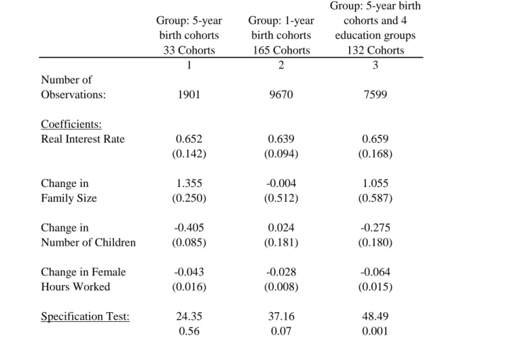
In order to give a robust picture of the role of precautionary saving in consumption growth, we report results for several different utility functions. First, σ and δ are es-timated by GMM using grouped panel-data and the time-series moments implied by the consumption Euler equation. Variables that shift the preference for consumption (Xi,t+1) include indicator variables for the month of the year to capture seasonal
varia-tions in demand. Since reported consumption declines slightly with each interview that a household participates in, preferences are allowed to vary by interview. We allow discount rates to differ by five-year birth cohorts. The number of family members and the number of children are both included because they shift the marginal utility of a given amount of expenditure. Finally, to control for the possibility that labor supply is non-separable from the marginal utility of consumption, the number of hours that the woman head of household works is included as a preference shifter. The intertemporal elasticity of substitution is estimated relatively precisely as0.652with standard error of 0.14, although there is also significant specification uncertainty. Appendix C describes the GMM estimator and estimates in greater detail. Having estimated the utility func-tion, it is possible that misspecification of preferences is minimal, so we present analyses of consumption growth with and without the correction for misspecification.22
The second approach is calibration. We analyze three different intertemporal elastic-ities of substitution: 0.3,0.65. and1(log utility). In each case we include no preference shifters, so that it is reasonable to believe that the misspecification adjustment is cap-turing preference variation. Therefore, as noted in section 3, the consumption growth due to misspecification is treated as consumption growth due to preference changes. For the decompositions based on estimation, the variation in consumption growth due to misspecification is omitted. In all cases, seasonal variation is removed.
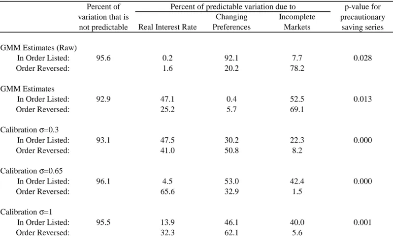
Table 1 shows, for our sample of unconstrained households, the share of variation in consumption growth due to innovations to consumption growth and the share of predictable variation due to preferences, the real interest rate, and precautionary saving. Before turning to predictable consumption growth, note that90percent or more of the variance of average consumption growth in the CEX is due to news or measurement error, evidence that we are not overfitting in predicting consumption growth. This large number stems from the fact that aggregate consumption growth is difficult to forecast with few instruments, and from the fact that measurement error in the CEX leads to unpredictable changes in average consumption growth.
Table 1 demonstrates that precautionary saving causes a statistically significant share of the volatility of expected consumption growth, and that there is a wide range of uncertainty concerning the economic importance of precautionary saving. Innova-tions to consumption growth are, by construction, orthogonal to the other components of consumption growth; however, the predictable series are not mutually uncorrelated. Therefore the share of variation due to any series depends on the ordering of the series in the variance decomposition. Table 1 presents two alternative orderings for each set of parameters. After the correction for misspecification, the GMM estimates of the per-cent of variation in predictable consumption growth due to precautionary saving range a concern as the estimates from this model are used to construct our measure of precautionary savings at an individual household level, rather than at the synthetic cohort level at which estimates of preferences were obtained. That the Euler equation holds for a synthetic cohort is necessary but not sufficient for it to be satisfied by an individual household.
from 2.5 to 95 percent. For the results based on calibration — which treat misspecifi -cation as preference variation — estimates of the economic importance of precautionary saving range from 1.4 percent to37percent. In contrast, the first row of results, which omit the correction for possible misspecification suggest that precautionary saving is far more economically important, directly causing 70 to 80 percent of variation in ex-pected consumption growth. But as emphasized in section 3, the presence of model misspecification inflates this measure by construction. The results with the correction for misspecification show that the importance of precautionary saving is significantly less, or at least more uncertain, when the predictable component of the error term is removed.23
Given this range of uncertainty, is there a statistically significant contribution of precautionary saving to the volatility of consumption growth? The last column of Table 1 reports the probability that there is no variation due to precautionary saving; that is the p-value for an F-test that the true coefficients in the regression constructing the expectation in equation (3.8) are all zero. Fluctuations in consumption due to precautionary saving are statistically significant in all cases except the raw residuals from GMM estimation.
The reason for the wide range of uncertainty over the economic importance of precau-tionary saving is itself informative. Expected consumption growth due to precauprecau-tionary saving is negatively correlated with that due to preference variation and positively cor-related with that due to movements in the real interest rate. These correlations are large, and this is what drives the uncertainty over relative importance. The positive covariance between consumption growth due to the real interest rate and that due to 23Also, comparing the second and fourth sets of results shows the effect of assuming that expected consumption growth due to misspecification is actually due to preference variation. The GMM esti-mates assume that estimated preferences capture all true preference variation and omit the misspecifi -cation series from the decomposition. The calibration assumes that misspecification captures omitted preference variation. When we include the misspecification as preference variation, the correlation of precautionary saving and preferences decreases and the role of precautionary saving is better pinned down.
precautionary saving implies that omission of the precautionary term from a regression of consumption growth on the expected real interest rate would increase rather than decrease the estimated elasticity of intertemporal substitution. We also find that con-sumption growth due to shifts in the preference for concon-sumption covaries negatively with that due to the real interest rate. Thus low observed intertemporal substitution in response to the real interest rate, as observed by Hall (1988) for example, is largely due to omitted preference shifters or misspecification of the consumption optimization problem more generally.24 Put differently, since precautionary saving leads to higher consumption growth when the interest rate is higher, precautionary saving cannot be the cause of low observed intertemporal substitution. This supports models in which expected changes in consumption growth are caused by nonseparabilities of nondurable consumption and home production, consumption of durable goods, or leisure.25
Table 1 also shows that the economic importance of precautionary saving is larger the larger the assumed level of household risk aversion and prudence. Lower values of σ, the elasticity of intertemporal substitution, imply a more important contribution of precautionary saving to predictable consumption growth. This occurs because σ also governs relative risk aversion (σ1) and relative prudence (1 + 1σ). A low elasticity of intertemporal substitution implies high risk aversion and high prudence.
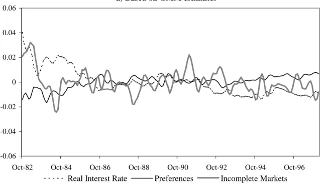
Figure 1 displays the three time series of expected consumption growth for both the GMM estimates and the calibration with σ = 0.65. The data are quarterly averages converted to annual rates, and apart from the series for preferences, are visually similar across panels. The primary difference between thefigures is due to the misspecification adjustment, which is included in the preference series in Figure 1b and omitted in Figure1a. There is a significant amount of predictable variation in consumption growth 24This supports one of the mainfindings of Attanasio and Weber (1995) and Attanasio and Weber (1993). These papers also argue that correct aggregation is an important part of the difference between linear models in micro and macro data.
25See Baxter and Jermann (1999), Ogaki and Reinhart (1998), and Basu and Kimball (2000) respec-tively.
“explained” by the nonstructural construction ofET,λ=0[εi,t+1|Zi,t],but unexplained by
the more structural utility function used in the GMM estimation.
In both panels, we see some evidence that precautionary saving has become less important over the sample, contributing less to consumption growth. This is consistent with the increase in wealth and economic boom of the1982−1997period and suggests that decreased risk has a role in the consumption boom (see Parker (1999)). We also see that risk contributes substantially to consumption growth after the large1982recession, consistent with consumption dropping in recessions due to increased consumption risk in the future. There is no similarly dramatic pattern observed around the 1991 recession, though consumption growth due to precautionary saving rises before the recession, and falls during and after it, with somewhat more accentuated movements in Figure 1b.
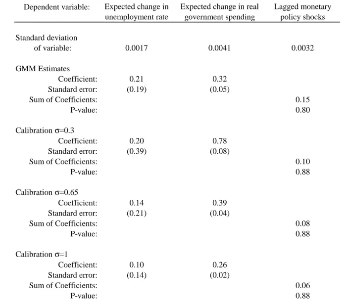
These are visual impressions. To be more formal, Table 2 presents the results of investigating precautionary saving by regressing expected consumption growth due to precautionary saving onto: the contemporaneous expected change in the unemploy-ment rate, the contemporaneous expected growth in governunemploy-ment spending, and lagged innovations to the federal funds rate.
The first column shows that precautionary saving leads to countercyclical expected consumption growth, although this is statistically insignificant. The point estimates imply that an expected one percent increase in the prime-age male unemployment rate is associated with 0.1 to 0.2 percent faster consumption growth due to consumption risk. The sign of the effect supports our theoretical understanding of precautionary saving — when the unemployment rate is expected to increase there is greater risk and therefore precautionary saving should be high and expected consumption growth should be greater.
The second and third columns of Table 2 present some reduced form evidence on precautionary saving and macroeconomic policy. Theoretically, there are two channels through which economists have considered policy changing consumption risk and pre-cautionary saving. First, expansionary policy can lead to less consumption risk, so that consumption increases when the policy is announced and then is expected to grow more
slowly over time. This effect is not consistent with the observed impulse responses of consumption to monetary policy shocks, for example, which show faster consumption growth for a while after a reduction in the real interest rate (Bernanke and Gertler (1995)). If instead policy is going to cause precautionary saving to increase consump-tion growth, it must be that expansionary policy leads to increased consumpconsump-tion risk. For example, if policy improves expectations of future income, households increase con-sumption on announcement reducing their stocks of liquid wealth, and this leads to higher consumption risk and faster consumption growth.26 To evaluate these theories, we ask how consumption growth due to precautionary saving responds to predictable movements in government spending and lagged monetary policy shocks.
An expected one percent higher growth rate of government spending is associated with a one-quarter to three-quarter of a percent faster consumption growth due to precautionary saving. This is consistent with pre-announced increases in government spending leading to faster consumption growth due to precautionary saving. As to monetary policy, we find no statistically significant relationship between consumption growth due to precautionary saving and 12lags of monthly monetary policy shocks as constructed by Bernanke and Mihov (1998), although the sign of the effect is positive, consistent with the impact of a monetary policy shock on total expected consumption growth.
In sum, wefind a statistically significant role for precautionary saving, some evidence that it has declined and is countercyclical, and conclude that its economic impact is both similar to that of the real interest rate and similarly uncertain in magnitude. We turn now from the sample of unconstrained households, in which we are studying the effects of precautionary saving, to the entire sample, in which our measure of consumption growth due to incomplete markets may include the impact of liquidity constraints.
26In models such as Carroll (1997), higher expected income growth leads to higher expected con-sumption growth through precautionary saving.
6. The proximate causes of consumption growth
This section presents the results from a similar set of exercises as the previous section, but performed on the data for all households. We find that expected consumption growth due to incomplete markets is directly responsible for a slightly larger share of consumption growth in the entire population than for only unconstrained households. Indeed, there is evidence that incomplete markets were a more important determinant of consumption dynamics in the1991recession for all households than for unconstrained households alone. Furthermore, consumption growth due to incomplete markets is more countercyclical for all households than for unconstrained households alone, and has no significant comovement with our policy variables. These results must be interpreted with care. There is a large negative correlation between expected consumption growth due to incomplete markets and that due to misspecification. The misspecification ad-justment induces significant movement in the incomplete markets series. The economic interpretation of this finding is that, for all households, preference shifters (or mis-specification) interact in important ways with incomplete markets. We give a concrete example below.
Table 3 presents the variance decomposition of consumption growth for all house-holds. Similar to the findings in the smaller, unconstrained sample, expected consump-tion growth due to incomplete markets is highly statistically significant. Slightly more than 90 percent of consumption growth is unpredictable. Unlike for unconstrained households alone, the corrected estimates from the GMM estimation (second set of re-sults) imply that precautionary saving and liquidity constraints together are directly responsible for a reasonably precise 52 to 69 percent of the predictable consumption growth. If however, one views all the predictable variation in the constructed expec-tation error as due to preferences then the measured effect of incomplete markets is smaller. The calibration results show a lower contribution of incomplete markets, and a greater level of uncertainty as to its role influctuations. As is the case for the uncon-strained sample, expected consumption growth due to precautionary saving negatively
covaries with that due to preference variation, and this covariance rises when “mis-specification” is included as preferences changes. Across specifications, the percent of variation in predictable consumption growth due to incomplete markets ranges from1.5 to 69percent.
Figure 2 displays the three time series of expected consumption growth for the GMM estimates (PanelA) and the calibration withσ = 0.65(PanelB). Again, incom-plete markets and the real interest rate each lead to similar fluctuations in consump-tion growth in each panel. Adding the misspecification correction to preferences in PanelB leads to volatile consumption growth due to changing preferences that is more negatively correlated with consumption growth due to incomplete markets. Why is this? One answer is simply thatET,λ=0[εi,t+1|Zi,t]is estimated only using unconstrained
households but used in the construction of∆lndCIM
t+1 for all households (equation (3.8)).
Statistically, the predicted values out of sample create this negative correlation. But a second answer is that there are good economic reasons for these predictions to be poor out of sample: constrained households are different. The presence of a binding liquidity constraint leads a household to adjust margins besides consumption and this can lead to exactly this type of negative covariance. For example, consider a young constrained household that increases labor supply in response to the constraint. As the constraint relaxes, labor supply declines predictably, leading to slower desired con-sumption growth due to preference shifts, while concon-sumption growth rises predictably due to the constraint relaxing. The large negative correlation suggests this is what is happening: preference shifters and liquidity constraints lead to offsetting movements in expected consumption growth.27 Given the magnitude of the negative correlation, we suspect the negative correlation is not purely due to economic behavior, but is also partly driven by imperfect prediction.
That said, like Figure 1, Figure 2 shows some evidence that precautionary saving and liquidity constraints have become less important over the time period covered by the data, contributing less to consumption growth. Comparing Figures 1 and 2, this
decline appears slightly larger for all households than for only liquid households. Also, liquidity constraints or precautionary saving of low wealth households seem to have played a role in maintaining consumption growth in the 1991 recession. Again, these are visual impressions. Table 4 reports the results of regressing consumption growth due to incomplete markets onto the same set of variables as Table2.
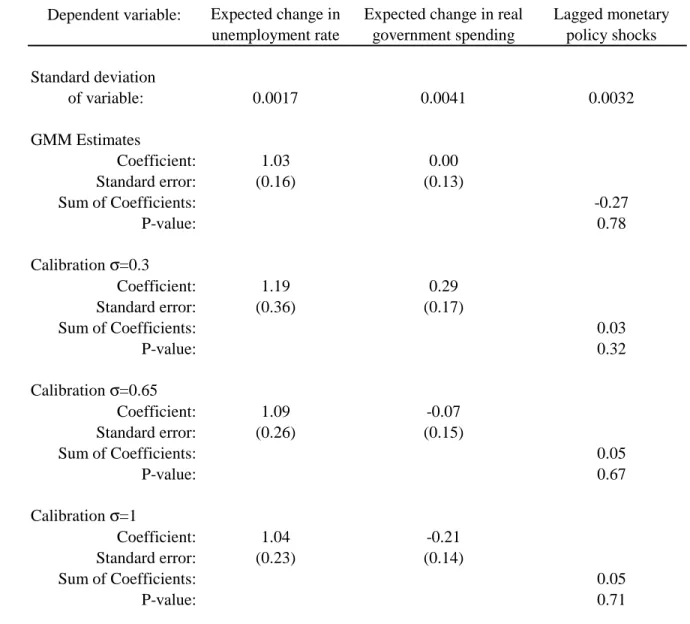
First, incomplete markets lead to countercyclical expected consumption growth. The point estimates imply that an expected one percent increase in the prime-age male unemployment rate is associated with just over a one percent higher rate of expected consumption growth rate. This effect is larger than that estimated for unconstrained households alone, implying that precautionary saving is more important for low wealth households. Larger increases in consumption risk for low wealth households could be due to the fact that unemployment falls more heavily on lower income households or that credit constraints are tighter when unemployment is expected to rise, so that borrowing to smooth consumption becomes more difficult. Either way, the estimates imply that incomplete markets amplify business cycle movements in consumption. Consumption risk increases and/or borrowing constraints tighten upon news of a coming recession and therefore incomplete markets for transferring consumption across time and states amplify the decline in consumption that occurs on this news.
The remaining columns of Table 4 show that both our measures of policy have insignificant correlations with expected consumption growth due to incomplete mar-kets. Unlike for unconstrained households, the impact is not consistently of one sign. There is no evidence that the combination of liquidity constraints and precautionary saving amplify or damp the impact of government spending or monetary policy on total consumption growth.
7. Conclusion
This paper proposes and implements a decomposition of consumption growth into its proximate causes. We show how the utility function and consumption data can be used
to source movements in consumption growth and demonstrate how to measure the role of precautionary saving in a manner robust to some misspecification. Using estimates and calibrations for a standard utility function, we implement this decomposition using the CEX survey data on household expenditures. In sum, we find that incomplete markets for trading future consumption cause statistically important movements in expected consumption growth and that the economic importance of precautionary saving rivals that of the interest rate.
For households that are unlikely to be liquidity constrained, expected consumption growth is sourced to movements in the real interest rate, changes in the preference for consumption, and precautionary saving. We find that the impact of precaution-ary saving on variations in consumption growth is statistically significant. While the magnitude is rather uncertain, the variance of predictable movements in consumption that are due to movements in precautionary saving is if anything slightly less than the variance due to movements in the real interest rate. There is some evidence, although imprecise, that precautionary saving is countercyclical, leading to higher consumption growth when unemployment rates are increasing. And there is some evidence that high expected growth in government spending is associated with greater consumption growth due to precautionary saving.
For average consumption growth, incomplete markets are more important forfl uctu-ations in expected consumption growth. Precautionary saving and liquidity constraints are highly statistically significant, and cause movements in consumption that are posi-tively correlated with movements due to the real interest rate and negaposi-tively correlated with movements due to preferences or “misspecification.” Consumption growth due to incomplete markets is countercyclical, and so amplifies recessions, but we find no evidence that it is correlated with past policy.
We suspect that measurement error in consumption growth limits our ability to infer the characteristics of consumption growth. Better measurement (or data in which with longer growth rates can be studied) would allow a tighter decomposition and a more accurate mapping from primitive shocks to subsequent movements in precautionary
saving. Better measurement may also allow analysis of trend growth rates. Of specific interest is the variation across countries in consumption growth rates, which are largely unexplained by variations in real interest rates. Our decomposition suggests a way to use microeconomic data to measure the differences in consumption risk across countries into implied differences in expected growth rates of consumption.
Appendixes
A.
The corrections to precautionary savingThis appendix demonstrates that the specification of the corrections described in section 3 are not interchangeable.
Consider first applying the correction for misspecification in the manner of the second correction. Assuming parameter estimates are correct apart from the misspecification termθ, the household-level measure of precautionary saving would be
−σI(1t) P i∈It ET [ln (1 +εi,t+1)−εi,t+1|Zt]. Since εi,t+1 = 1 + i,t+1 θi,t − 1
the expectation of this measure is equal to
−σE · ln µ 1 + i,t+1 θi,t ¶ −1 + i,t+1 θi,t + 1 ¸
= −σE[ln (1 + i,t+1)]−σ(−lnθi,t+
1 θi,t
+ 1).
Expanding the second logarithm around θi,t = 1, one can see that this measure is correct to
the first order but not higher. Under this alternative, θi,t raised to powers would show up in
our measure of precautionary saving.
Turning to the correction for small-sample bias, suppose that we were to subtracteˆt+1 ≡
ET h 1 I(t) P i∈Ite˜i,t+1|Zt i
from the residual in the manner of the adjustment for misspecifi ca-tion, so that the measure of consumption growth due to precautionary saving is
−σET · 1 I(t) P i∈It ln (1 + ˜ei,t+1−eˆi,t+1)|Zt ¸ .