NBER WORKING PAPER SERIES
BEQUEST AND TAX PLANNING:
EVIDENCE FROM ESTATE TAX RETURNS
Wojciech Kopczuk
Working Paper 12701
http://www.nber.org/papers/w12701
NATIONAL BUREAU OF ECONOMIC RESEARCH
1050 Massachusetts Avenue
Cambridge, MA 02138
November 2006
I benefited from comments from anonymous referees, the editors, participants of seminars at the 2004
meeting of the National Tax Association, 2005 NBER Summer Institute, Columbia, Michigan, Wisconsin
and Virginia, as well as from discussions with David Forrer, Joel Slemrod, Till von Wachter, Karl
Scholz, Emmanuel Saez and David Joulfaian. Financial support from the Program for Economic Research
at Columbia University and the Sloan Foundation is gratefully acknowledged. The views expressed
herein are those of the author(s) and do not necessarily reflect the views of the National Bureau of
Economic Research.
© 2006 by Wojciech Kopczuk. All rights reserved. Short sections of text, not to exceed two paragraphs,
may be quoted without explicit permission provided that full credit, including © notice, is given to
the source.
Bequest and Tax Planning: Evidence From Estate Tax Returns
Wojciech Kopczuk
NBER Working Paper No. 12701
November 2006
JEL No. D12,D31,D91,H2
ABSTRACT
I study bequest and wealth accumulation behavior of the wealthy (subject to the estate tax) shortly
before death. The onset of a terminal illness leads to a very significant reduction in the value of estates
reported on tax returns - 15 to 20% with illness lasting "months to years" and about 5 to 10% in case
of illness reported as lasting "days to weeks". I provide evidence suggesting that these findings cannot
be explained by real shocks to net worth such as due to medical expenses or lost income, but instead
reflect "deathbed" estate planning. The results suggest that wealthy individuals actively care about
disposition of their estates, but that this preference is dominated by the desire to hold on to their wealth
while alive.
Wojciech Kopczuk
Columbia University
420 West 118th Street, Rm. 1022 IAB
MC 3323
New York, NY 10027
and NBER
1
Introduction
This paper provides empirical evidence about behavior of wealthy individuals following the onset of a terminal illness using (publicly available) individual-level estate tax return data (National Archives and Records Administration, 1995) for decedents whose tax returns were filed in 1977. This is the only publicly available dataset of this kind and one of very few data sources allowing to study wealth holdings and behavior of the wealthy.1 I analyze decisions of estate taxpayers shortly before their deaths. My strategy is to compare estates of individuals who suffered terminal illnesses of different lengths. Approximately 20% of taxpayers subject to the estate tax die instantaneously. The central empirical fact established in this paper is that their estates as reported on tax returns are 10-18% greater than estates of those who suffered from a lengthy illness. This could be consistent with large medical or long-term care expenses or with loss of income following the onset of a terminal illness. However, based on other information from tax returns and AHEAD/HRS exit surveys I show that these are unlikely to be the right explanations. Instead, the empirical findings suggest that this response reflects planning for the disposition of an estate.
While the notion that the wealthy pursue tax avoidance is hardly new or surprising, the results shed a new light on motivations behind wealth accumulation. The presence of significant tax-motivated actions following the onset of a terminal illness reveals a desire to control disposition of assets, but it also implies that more tax planning could have been pursued earlier. Tax avoidance is easier and more effective if pursued early. Furthermore, those who die instantaneously do not get a chance to make such adjustments. This suggests that there are real costs to early planning that result in holding on to wealth while alive and that (rational or irrational) “procrastination” in estate planning is an important phenomena. I present additional findings that are consistent with the notion that the wealthy hold on to their wealth until they die: in cross-section wealth is increasing with age until the maximum observed age of ninety-eight. Because cross-sectional wealth profiles are potentially affected by differential mortality, these findings do not unequivocally prove that wealth increases with age. Still, the sample considered is more uniform than usual so that selection is less likely to be an issue and, despite that, the gradient is steeper (estimated at approximately 3% per year) than observed in datasets representative of the full population. Together with bequest-driven adjustments before death, these patterns cast doubt on the life-cycle motive for wealth accumulation as the sole explanation of behavior of the wealthy.
The results suggest a need for a model that can simultaneously explain wealth accu-mulation beyond own consumption or precautionary needs, some degree of concern about beneficiaries and significant delays in planning despite real consequences. Holding on to wealth until one gets terminally ill despite tax consequences suggests a “capitalistic spirit”
1The analysis uses individuals with estates of at least $120,000 in 1976, corresponding to roughly $360,000
nowadays. The group considered corresponds to approximately 6% of adult deaths. Information on more than 29,000 high net worth tax returns is in the data vastly exceeding the coverage of this group in any survey dataset. Sampling rates are also higher and the effective exemption level is lower than in any of the more recent IRS samples of estate tax returns (that are not available publicly). I discuss the data in more detail in Section 2.1.
or wealth in utility motive where wealth accumulation takes place because stock of wealth provides flow of utility. The presence of active though delayed planning suggests however that such a framework will not fit all empirical facts. An alternative is for individuals to simultaneously value both wealth and bequests. It is natural to expect that the presence of such a preference that’s ultimately reflected in tax-motivated actions should affect wealth accumulation prior to the onset of a terminal illness, although results in this paper leave open the possibility of “lexicographic” preferences under which wealth accumulation has nothing to do with beneficiaries yet transfers to them are preferred to transfers to the IRS. Another important possibility for explaining my findings is behavioral: individuals who have difficulty acknowledging their own mortality may delay planning and oversave.
Other than establishing the drop in net worth, I find that the response is stronger for younger individuals and that administrative expenses associated with the estate fall. I also show direct evidence of increased planning: transfers before death increase, although this response does not reflect simple direct inter vivos giving but rather it reflects more complicated transfers that are pre-arranged but take effect only at the time of death.2 Such transfers are likely to be a fingerprint of more sophisticated avoidance strategies that are not directly observed on the tax return. Consistent with a tax motive, I find that the response for a subset of individuals who died in 1977, following a tax cut that took place on January 1st 1977, is much weaker.
I find no evidence that these wealthy taxpayers experienced any quantitatively important financial hardship due to lost income. I also find no evidence that debts increase suggesting that taxpayers do not experience difficulties dealing with terminal expenses. I discuss other evidence suggesting that while end of life expenditures are important for most of the population, they have very low wealth elasticity and are not of major importance at the top of the distribution. As far as I know, this is the first paper that documents low wealth elasticity of terminal expenditures. This information is not observed on the tax returns and therefore I rely on AHEAD/HRS surveys to shed some light on this issue. I find that medical, funeral and related expenditures in the last two years of life for individuals who would meet the estate filing threshold in my data (roughly $360,000 nowadays) constitute at most 4% of estates (they are on average 45% for the full sample) and do not show a strong gradient with respect to the length of illness. In particular, these expenditures are much smaller than the estimated effects and thereby cannot explain the drop in net worth. Finally, I document changes in the allocation of assets. Interestingly, I do not find a disproportionate decrease in cash holdings perhaps reflecting no outright tax evasion, but also consistent with income from sales of other assets offsetting any cash distributions. That cash holdings do not fall disproportionately is another argument against the relevance of any liquidity-related problems. One indication that outright cheating may be facilitated by a longer illness is that the category of “other assets” responds strongly for smaller estates. Items specifically mentioned on the tax return that fall into this category are jewelry, furs, paintings, antiques, rare books, coins and stamps and household goods: these are, likely,
2
As an example, an outright transfer of a house would be an inter vivos gift, but a transfer of a house with retained right to use it until death is a lifetime transfer and should be included on the estate tax return.
things that can be easily concealed from a tax collector. For those with moderate wealth (who would not be subject to taxation in 2005), I find evidence that farms and business assets disappear or lose (reported) value following the onset of a terminal illness. This is no longer true for higher net worth individuals, but for all categories I find that corporate stock (the category that includes closely held corporations) responds strongly.
The econometric analysis of the data from estate tax returns is complicated due to the presence of truncation: only estates that are larger than filing threshold are observable by the researcher. To my knowledge, this is the first paper taking this issue seriously and I find that addressing that the data comes from a truncated sample affects the results significantly. I rely on a number of different methods to deal with truncation and find that results are robust to these approaches. I use both parametric and semi-parametric methods that require weaker distributional assumptions. I also rely on availability of information a few years before death to define subsamples on which truncation is less severe and verify that the results are robust to this approach as well.
The plan of this paper is as follows. In Section 2, I discus the data and present my econometric strategy. Section 3 analyzes the response of net worth to the length of illness and section 4 discusses channels behind this response. Conclusions are in the final section.
2
Data and econometric strategy
2.1 Data
I rely on the Decedent Public Use File (DPUS) available from the National Archives and Records Administration (1995). This dataset was constructed by linking information from four sources: the SSA 10% Continuous Work History Sample “decedent” file that includes deaths that occurred between 1974 and June 1977, the IRS Statistics of Income sample of estate tax returns filed in 1977 and both 1969 and 1974 IRS Individual Master Files comprised of income tax returns filed in 1970 and 1975 respectively.3 I limit attention to estate taxpayers (I do not observe estates of others) and use information from their 1977 estate tax returns and income tax returns for 1969 and 1974.
The dataset contains information about 40462 estate tax returns. This is a stratified sample that includes 100% of 1977 returns with gross estates above $500,000, 20% of returns between $200,000 and $500,000, and 12.5% of returns with gross estates below $200,000. In all reported specifications I weight observations by the inverse of sampling probability. The threshold for estate filing increased in 1977 from $60,000 (gross estate) to $120,000.4 I use net worth constructed by subtracting debts from gross estate as the criterion for sample selection. Net worth is necessarily smaller than gross estate and therefore all individuals
3The link with the CWHS is not important for this paper. Its main purpose in creating this dataset was
to identify deaths for non-estate taxpayers. The variables from the CWHS present in the dataset are race, sex and age (the latter two would be observable for estate taxpayers anyway) but unfortunately earnings information (which is present in the SSA version of the CWHS) is not included.
4
with net worth above the gross estate filing threshold were subject to the filing requirement.5 There are 29,407 observations with net worth above $120,000 drawn from the universe of 112,600 deaths (obtained as the sum of inverse sampling probabilities). The numbers of adult (21 and up) deaths in each of 1976 and 1977 were around 1.8 million so that the data corresponds to about 6% of all adult decedents. Thus, this group includes a fairly broad segment at the top of wealth distribution. In particular, it is significantly broader than those subject to estate taxation nowadays, or at any period other than the 1970s. I will also show, therefore, results for those with net worth greater than $500,000 (in 1976 dollars) that corresponds to a little more than the 2005 estate tax threshold of $1.5 million.6
Estate tax return data are very detailed and contain information about the composition of estate, deductions, some additional schedules, tax credits etc. as well as age, marital status and gender. Individual income tax data contain a few basic variables such as the adjusted gross income, wages and salaries, dividends and interest, information about ex-emptions claimed and a few additional items. There is no information about the state of residence (other than community/non-community property state distinction) and the ex-act date of death. It is possible to ascertain whether death occurred in 1977 or earlier by comparing the tax liability reported in the data to the size of taxable estate.7
For the most part, the analysis will be limited to married males. In the considered period married male decedents were subject to heavier taxation than now. The unlimited marital deduction was not introduced until 1981. Up until 1976, 50% of the estate was deductible. Starting in 1977, the marital deduction was increased to the larger of $250,000 or 50% of the estate. Therefore, married male decedents were subject to taxation in the period covered by the data, but the tax treatment changed between 1976 and 1977.8 Responses of different marital and gender groups are likely different because their circumstances are different: for example, any decision of a widow is observed only after her husband died. On the other hand, response of a married person needs to take into account that there may be additional adjustments by the surviving spouse. As a result, different groups should be considered separately. As will be discussed below, the information about 1969 income of an individual is important for the analysis. While information about 1969 Adjusted Gross Income (AGI)9 is in the data for 92% of men, it is missing for 48% of women. This is particularly common
5
This eliminates less than 0.5% of returns with gross estate above the threshold but net worth below.
6The data captures the population that is hard to observe in conventional survey data. The only large
survey that oversamples high wealth population is the Survey of Consumer Finances which is a cross-section of the living population, and therefore does not allow for studying implications of increased mortality risk (and, despite its oversampling of the wealthy, it does not approach the sample size available here).
7
I was able to perform limited tabulations on the same estate tax return data held at the SOI (but without the link to income tax returns) and obtain information about the distribution of dates of deaths for this sample. 6169 deaths occurred in 1977, 32459 in 1976, 1345 in 1975, 239 in 1974 and 250 prior to that.
8
Two other important tax changes took place in 1977: gift and estate taxation were integrated and rules regarding transfers made within three years of death changed. I make very limited use of the 1976 tax reform, because I observe estates of individuals who died in 1977 only if they filed in 1977, i.e. if the tax return was filed relatively quickly. This is then likely to be a selected sample. More details are in section 3.
9Adjusted Gross Income (AGI) includes all types of income subject to income tax as reported on the
tax return (wages and salaries, interest income, dividends, business income, capital gains etc.) less a few (usually very small) adjustments to income.
for married females (most likely, because data matching relied on primary filer’s SSN only), but even among widows it is still the case for 42% of the sample — possibly because their husbands were still alive in 1969.10 As a result, incorporating women in the analysis is difficult both due to much smaller sample sizes and possible selection issues.
2.2 Length of illness measure
The key variable for the identification strategy of this study is the length of terminal illness. This information is available in the dataset as a categorical variable that takes ten values: instantaneous (minutes), hours, 1 to 3 days, 4 to 7 days, 8 days to less than a month, 1 to 3 months, 4 to 6 months, 7 months or less than a year, 1 to 9 years and more than 10 years. I aggregate these values into three categories: “quick” (instantaneous), “medium” (hours, days or weeks) and “long” (months or years),11 and study differences in behavior across groups defined by these categories.
Basic summary statistics by the length of terminal illness for the sample of married males are shown in Table 1. Some variables vary with the length of illness. Those dying instantaneously are younger than others. Such deaths are also less common in the 1977 subsample (as discussed below, it may be due to selection on the delay in filing a return). There is also a bit of a difference in income a few years earlier. This issue will be discussed below. A few financial variables appear quite different across categories. There is some difference in the size of net worth, stocks, bonds, real estate and life insurance. Strikingly, there is a major difference in assets reported on the Schedule G — “lifetime transfers.”
Length of illness is based on response to the item #4 “Length of last illness” in the “General Information” section of the estate tax return. There is no guarantee that this question has always been answered accurately,12,13so that one may worry about the quality
10Information about income tax return for 1974 is missing for 28% of widows.
11
This aggregation helps in reducing the extent of misclassification and keeping the number of reported
coefficients manageable. Note that the distinction between immediate deaths and longer term illnesses
is likely to be much cleaner than between other categories. This motivates separating the instantaneous category from any longer illness: it is likely to be dominated by unexpected events (ideally, from the identification point of view, it would reflect purely random accidents), while even a short-term terminal illness may be the result of a known pre-existing condition. A misclassification error will act against finding an effect. The results are noisier but robust to finer measurement of the length of illness.
12
16.2% of the sample does not contain an answer to this question at all. These individuals are more commonly widowed, single or divorced and they are younger than average. There seem to be no selection based on net worth or income. Inaccuracy would also likely be an issue in any survey data. HRS/AHEAD includes an exit survey that contains such information, but it has few high-wealth individuals. In either case, it is of course someone else (the executor of the estate in the estate tax case, a family member in surveys) who responded to this question.
13
One reason for misleading answers has to do with tax avoidance: transfers made in “anticipation of death” had to be included in the estate and this could provide an incentive to hide a lengthy illness. Transfers within three years of death were presumed to be in anticipation of death and the burden of proof that it was otherwise fell on the taxpayer. If such transfers were present, the executor was required to provide information about hospitals in which the taxpayer was confined in the last three years of life. While it is not possible to measure the extent of this problem, it acts against finding an effect of the terminal illness, because it shifts tax avoiders experiencing a large response to the non-treatment group.
of this variable. In Table 2, I show how length of illness varies with age and gender. Instantaneous deaths become less common with age and they are more common for men than women, with the difference shrinking with age. This pattern seems reasonable and is consistent with this variable containing information about the actual length of illness.
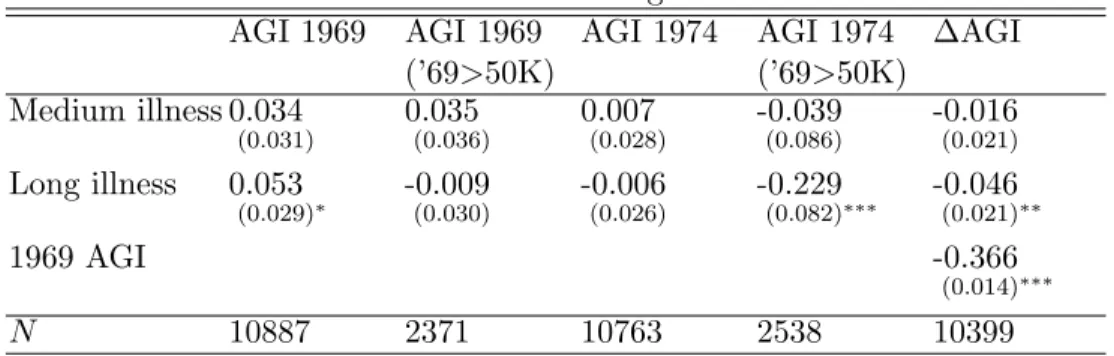
A more direct tests of the informativeness of this variable can be obtained by regressing income a few years before death on the length of illness. Table 3 shows the results.14 The simple regression of 1969 AGI on the length of illness produces a perverse positive coefficient on the lengthy illness. Note though that this is actually consistent with the effect of truncation (only estates greater than $120,000 are observed) in the presence of an effect of illness on net worth: when those suffering from lengthy illness die with lower net worth, some of them drop out of sample. Because wealth is strongly correlated with AGI, this leads to eliminating from the sample some relatively low AGI individuals who suffered from a lengthy illness, thereby increasing the truncated sample mean of AGI conditional on long illness. Consistently with this story, the effect disappears when the sample is restricted to those with 1969 AGI greater than $50,000 — a subsample where truncation is less important. When a similar exercise is repeated using 1974 AGI, estimates for the full sample are no longer positive and the effect of lengthy illness for the subsample of those with 1969 AGI greater than $50,000 is large, negative and significant. This suggests that individuals who suffered from a long illness already experienced a drop in income as of 1974. Comfortingly, the coefficient on medium illness is very close to zero: such an illness should not yet have had its onset as of 1974. The final column reports the results of regressing the change in AGI between 1969 and 1974 on the length of illness, while rudimentarily controlling for truncation by including 1969 AGI in regression (this strategy is further discussed below). This specification again suggests that income fell by 1974 for those who suffered from a lengthy illness. Overall, the fact that 1974 AGI responds to lengthy illness but 1969 AGI does not is supportive of the length of illness containing real information. Furthermore, the difference between results for full and restricted samples is suggestive of the presence of an effect of the length of illness on net worth that leads to selection effect due to truncation.15
2.3 First stage — truncation
The econometric objective is to measure the impact of terminal illness on net worth and other variables reported on tax returns. Denote byWi the value of net worth of individual
i, by Di the indicator(s) of the length of terminal illness and by Xi values of any other
relevant control variables. I assume the following relationship:
ln(Wi) =γDi+βXi+εi (1)
14
Third degree polynomial in age is included in all regressions but coefficients are not reported in tables.
15When AGI was decomposed into available components, similar (albeit usually insignificant) effects of
and I am interested in estimatingγ. Two econometric concerns need to be addressed. First,
Wi is observed only if an estate tax return is filed. I observe (Wi, Di, Xi) only when:16
Wi > T (2)
whereT is the threshold for inclusion in the sample (T is $120,000 for the whole sample but I will also consider truncating the sample at higher thresholds). As a result, this is an example of a truncated regression (the difference between this setup and a more common censored regression is that here individuals with wealth below the threshold are not observed).
Directly comparing distributions of wealth under truncation is difficult. A simple pro-portional effect may shift the conditional density at the truncation point up or down. One can also show that it is possible for a factor to reduce wealth and yet for the average wealth above the threshold to increase: some low wealth individuals then fall below the threshold and are no longer used to construct the average net worth above it.17 Identification in problems with truncation is harder than in problems with censoring: the extra information about the number of people who drop below the threshold available under censoring makes it feasible to adjust for this effect (see Powell, 1994, for a discussion). Such information is not available (at least not directly) here: one does not know how many individuals with given characteristics (critically, with the given length of illness) are located below the threshold. Second, in general, the distribution of the error termεi is not known. If the shape of the
distribution was known, the maximum likelihood approach would be straightforward. It is well known that the upper tail of the wealth (and income) distribution has “thick tail” and it is usually well approximated by the Pareto distribution. When the set of regressors (Di, Xi)
includes only variables that are bounded (e.g. categorical variables such as gender or marital status or variables with bounded support such as age),γDi+βXi must be bounded as well
and therefore thick tails ofWi must correspond to thick tails of εi. As a result, standard
approaches to Tobit-like models relying on normality or transformations to normality are unlikely to be appropriate. Most of the observables belonging to specification (1) are in fact bounded. All variables with infinite support observable on the estate tax return are potentially related to Di and therefore should not be included. This is where the link
with income tax returns is crucial. I will include income a few years prior to death in specification (1). The idea is that conditional on income (that is known to have a distribution with thick tails as well), estates may be more normally distributed. As a result, it is then possible that the normality assumption is not severely violated, in particularγDi+βXi no
longer needs to be bounded because it includes regressors with full support.
This parametric assumption will be investigated further. The Pareto distribution could be an alternative parametric candidate, but despite it being a good approximation for the
16
The only variables not observable whenWi is below the threshold areWiand Di. AllXi’s that I rely
on are present either on income tax return or in the CWHS. I do not use this source of information.
17
A simple example illustrates it: consider a threshold of $120,000 and two individuals with net worth of $130,000 and $270,000, respectively. The average net worth above $120,000 is equal to $200,000. Consider a 10% decrease in net worth for both individuals. The first individual falls below the threshold, making the conditional net worth above the threshold equal to the net worth of the second person — $243,000: the observed average net worth increases by more than 20% despite a 10% drop in net worth for everyone.
tails of income and wealth distributions, there is no guarantee that it describes well the overall distribution of the error terms conditional on regressors. In particular its validity for the upper tail does not imply validity at lower wealth levels. Since maximum likelihood estimates from the Tobit-style models are inconsistent when the distribution is mis-specified, I consider semi-parametric techniques that impose weaker distributional assumptions.
A number of semi-parametric estimators have been proposed in the literature. I apply Powell’s (1986) symmetrically censored LAD and symmetrically censored least squares to make sure that my results are not driven by the parametric assumptions. These estimators assume that the distribution ofεi is symmetric. This is a weaker assumption than
normal-ity although it is not necessarily compatible with “thick tails.”18 These methods impose artificial truncation from above to make the distribution of error terms in the sample used in estimation symmetric. As a result, they effectively rely only on a subset of observations. The extent of this additional truncation depends on the variance of error terms and, as a result, inclusion of additional regressors increases the number of effectively used observa-tions. Therefore, one should use them even if they could be omitted (i.e. when they are orthogonal to other regressors). Thus, it turns out that inclusion of prior income is critical also for the semi-parametric approaches even though it does not appear to be correlated with the length of terminal illness.
Another possible approach is to estimate equation (1) on a subsample for which the condition (2) always holds. In such a subsample equation (1) could be estimated by ordinary least squares. Clearly, the required condition is the selection of a subsample in a way unrelated toε. I will rely on subsamples defined using income in 1969. Given that net worth at death is highly correlated with lifetime income, focusing on observations with high enough income reduces (though does not eliminate) the incidence of truncation. Furthermore, directly controlling for income in equation (1) deals with a concern about the selection bias from this procedure. Results of the robustness analysis are reported in Appendix A.
There are three classes of reasons why net worth may vary with the length of illness. First, there may be factors simultaneously affecting net worth and the length of terminal illness. An example of such a factor is age: net worth is likely a function of age in the sample due to both cohort and life-cycle effects. Observable factors of this kind can be controlled for. Unobservable factors driving both the length of illness and pre-illness net worth are a caveat to this analysis. The logarithm of 1969 income may be interpreted as a measure of socio-economic status, thereby addressing the potential bias if the length of illness and wealth were both driven by socio-economic factors varying within this sample.19 Second, attrition from the sample may be correlated with the length of illness. As an example, suppose that individuals with net worth slightly above the filing threshold (or
18Honore and Powell (1994) pairwise differenced LAD and least squares approach does not require
sym-metry but instead imposes independence of regressors therefore precluding heteroskedasticity. It is compu-tationally intensive, with a naive algorithm requiring evaluation of the objective function for each pair of
observations (i.e., the computation cost of the order ofn2, for more than 10,000 observations used here it
requires evaluating 50 million terms). Details of an algorithm with the cost ofn·log(n) are available from
the author, however even with that adjustment the approach turned out too computationally burdensome.
their families) do not realize that they are subject to the filing requirement. If those who get sick contact an estate planner, they may become informed and file a return even if they otherwise would not. The differential extent of non-filing cannot be directly tested, but it should become less of an issue as one moves up in wealth distribution. Third, there may be a direct causal relationship between net worth and the length of illness. The maintained assumption is that it is the length of illness that causes net worth and not the other way around.
2.4 Second stage — incidental truncation
Gaining insights into the nature of responses will involve analyzing information other than net worth that is available on estate tax returns. Denote a particular variable of interest by
Yi. Examples of such variables are charitable contributions, various asset holdings (stocks,
bonds, life insurance, cash) and the amount of lifetime transfers. Yi is potentially affected
by the length of terminal illness as well as being affected by other control variables:
Yi =δDi+ψXi+ηi. (3)
The nature of the data again does not lend itself to a simple least squares approach. First, as before, (Yi, Di, Xi) is only observed for individuals who file an estate tax return.
There-fore, the fully specified econometric framework should involve the three equations: (1), (2) and (3). This setup is different than the common Heckman-style selection problem. What is observed is not just a binary selection indicator but the selection variable (Wi) itself. Such
a framework is known as “Tobit Type-3” or “incidental truncation” model. As pointed out by Lee (1982) and Wooldridge (2002), observability of the determinant of selection has one crucial advantage relative to the Heckman-style selection framework: identification does not require an exclusion restriction in equation 1. To see why, observe that the selection problem is due to conditioning onW > T. When specification 3 is conditioned onW > T, the error term does not disappear but remains as E[η|X, D, W > T]. The standard two-step selection correction amounts to constructing this nuisance term. In the binary-selection framework, this construction relies on regressors from the first stage and therefore identification of (δ, ψ) requires that at least one of the second-stage regressors does not underlie the construction of the correction term (unless one is willing to rely on nonlinearity of the correction term). With a Tobit-style selection equation (either censored or truncated), the observable selec-tion indicator provides an extra source of variaselec-tion that allows for an addiselec-tional degree of freedom in the selection correction procedure and thus it allows identification of the param-eter of interest without an exclusion restriction (see Wooldridge, 2002, page 572). This is very convenient, because there is no natural exclusion restriction here.
In the main approach relied on in this paper, it is assumed that E[η|D, X, W] = αε. A sufficient condition is that (ε, η) are jointly normal, but it is a weaker requirement than that. If that this is the case, the conditional mean E[Y|D, X, W] is given byδD+ψX+αε. Althoughεis not observed, it can be consistently estimated using the truncated regression approach and this estimate of the residual can be used in the second stage in place of ε. This estimate varies independently of X and D because of its dependence on W. Note
that while the first stage estimation assumes normality, the second stage only requires the assumption that the conditional mean ofη on regressors is linear inε.
I also consider relaxing the parametric assumptions. I rely on three semi-parametric methods. Chen (1997) and Honore et al. (1997) proposed two-stage estimators for Tobit Type-3 models. First, the truncated or censored selection model is estimated. I will rely on the symmetrically censored least squares estimator. In the second stage, one of the Chen (1997) estimators (referred to as “Chen #1”) and the Honore et al. (1997) estimator use sample restricted so that the selection term is constant.20 The other of the Chen (1997) estimators (“Chen #2”) amounts to a non-parametric construction of the residual term. Its advantage is that it effectively brings into estimation all of the observations.
I construct standard errors by bootstrapping the whole two-step procedure 1000 times. The final issue concerns the functional form specification. I use logarithms of net worth and AGI. This approach reduces the influence of outliers and makes it easier to assume homoskedasticity, which is implicit in a normal truncated regression. In the second stage, some variables involve a non-trivial number of observations with zero values. To incorporate them, I considered four approaches. First, in my main approach, I use the logarithm of one plus the dollar amount. Second, for variables that have a significant number of observations at zero, I assume normality and run a tobit on the whole sample using logarithms of the dependent variable censored at $1000.21,22 Third, I take the share in net worth as the dependent variable. Fourth, I run a linear probability model for the presence of the asset.
3
The effect of illness on net worth
I begin with OLS that ignores truncation. Such results are biased toward the opposite sign and thus provide the lower bound for the extent of decrease in net worth due to longer illness. As shown in the first two columns of Table 4a, the simple regression yields a negative and significant effect of the length of illness on the size of net worth. The estimated effect is 5 to 6.5% decrease in response to a long terminal illness, depending on whether 1969 AGI
20
The Chen #1 estimator uses only observations that in the first stage were lying above the regression line and for which the truncation point is below the estimated regression line. If the distribution of error terms conditional on observables is independent of observables, the selection term is then constant in this subset. Honore et al. (1997) rely on symmetric trimming to guarantee the same condition. Their estimator is consistent in the presence of heteroskedasticity as long as the distribution remains symmetric.
21The $1000 threshold is chosen arbitrarily. For almost all variables there are very few observations with
values between $0 and $1000.
22
The advantage of the first approach is that it makes no additional assumptions about the second stage error terms. In the absence of a response on the extensive margin (the presence of an asset), it has a similar interpretation as the standard logarithmic specification. Otherwise, it also accounts for the response on the extensive margin. Given that such a response involves a change from the logarithm of the actual dollar value to zero, while the response on the intensive margin is approximately equal to a percentage change, the extensive margin response can be measured as large even though dollar amounts are small. This potentially large weight put on the extensive response must be taken into account while interpreting these estimates. The results from the Tobit approach have the standard interpretation, but it assumes normality in the second stage. In practice, results are qualitatively and quantitatively similar, suggesting that the response on the extensive margin does not affect the first approach in a major way.
is controlled for. These and all subsequent specifications include also a third degree age polynomial and a dummy for dying after 1976.
The second approach is the truncated regression model assuming normality and esti-mated using maximum likelihood. The results with and without controlling for 1969 AGI are shown in the second panel of Table 4a. They show a stronger effect of net worth than in the case of OLS. When previous AGI is controlled for, the estimated effect of the lengthy terminal illness is−.18 and it is also negative (−0.11) for the medium term illness.
The results also show that controlling for 1969 AGI plays a significant role. The effect of a lengthy terminal illness without controlling for the 1969 income is−.411 and the effect of the middle-length illness is then −.219 — these estimates are twice as big as the ones obtained when 1969 AGI is controlled for. What is the explanation of the role that AGI plays? There could be two possible reasons. It is possible that the length of illness is related to income. If that is the case, permanent income would be a joint determinant of net worth and the length of illness. This would be a reason for having 1969 AGI as a control but it would also be discomforting, because 1969 AGI is at best a noisy measure of permanent income making it difficult to argue that all such influences are controlled for. Second, 1969 AGI may be relevant because its inclusion changes the distribution of the error term and the distributional assumption is embedded in the estimation method. As shown in Table 4a the latter is most likely the case: when the length of illness variables are excluded, the coefficient on the 1969 AGI does not change, suggesting no relationship between the length of illness and prior income. Since inclusion of AGI affects estimated coefficients in the truncated regression specification, it indicates that this variable plays an important role in affecting the shape of the distribution of the error term.
Credibility of the truncated regression estimates rests on the credibility of the distribu-tional assumption regarding the error term. As argued before, when net worth is studied the normality assumption is plausible when one conditions on income but not otherwise. The results based on the truncated regression with 1969 AGI are the preferred specification. Results are robust to other approaches to truncation, details are presented in Appendix A. Table 4b shows the results using different truncation thresholds for net worth: $250,000, $500,000 and $1 million. The purpose of this exercise is to evaluate the possibility of heterogeneous responses for different net worth categories. These results are quite stable. In particular, the normality-based truncated regression with either $250,000 or $500,000 threshold are only a little bit weaker than the results for everyone above $120,000. Estimates for those above $1 million are weaker and insignificant (but the sample is much smaller) although still negative. The last two columns are based on the sample is artificially truncated from above, while accounting for this second layer of truncation in the likelihood function. The results indeed appear to become weaker as net worth increases, although they remain negative. One interpretation consistent with these results is that individuals with larger net worth have done more planning beforehand so that less needs to be done shortly before death. Another possibility is that inducing the same proportional change in a large fortune shortly before death is harder than in a small one.
As discussed before, most of the observations correspond to deaths before 1977, but there are also some observations for 1977. Taxation of estates changed in 1977: marital deduction was extended to cover at least $250,000 (or 50% of adjusted gross estate, whichever was greater) and the tax exempt amount was also increased. The extension of marital deduction was particularly important and the number of non-taxable estates among married males with net worth greater than $120,000 increased from 5.4% among pre-1977 deaths to 72.4% in 1977 (though the marginal tax rate for non-spousal transfers often remained positive). As a result, it is likely that individuals dying post 1976 behave differently than those who died earlier. The first panel of Table 4c shows results for the pre-1977 population, while the second panel shows results for 1977 decedents. Results prior to 1977 are very consistent with previous conclusions, in fact they are even somewhat stronger. Estimates for 1977 tend to be insignificant. The disappearance of response after 1976 is consistent with 1977 decedents pursuing less planning following the onset of a terminal illness due to weaker tax incentives to do so.
The caveat to the interpretation of the difference in results for the pre-1977 and the 1977 data is non-random sample selection. Individuals who died in 1977 are in the sample if their tax returns were filed in 1977 and not later. It may be that early filers are simply good planners and therefore there is no response. Alternatively, more complicated estates with higher net worth may be filed late but this effect might be weaker in situations when death was expected and significant planning has already taken place. In fact, in the pre-1977 population, 21.1% of individuals were reported as having died within hours while the corresponding number for post-1976 population is 17.8%. The gap increases to 4.9% for those with net worth above $1 million.23 Whether this gap is due to selection or whether it reflects a response of estates to the length of terminal illness24 is however non-testable. The potential sample selection problem makes it difficult to study the effect of the 1976 tax reform using this dataset and it is the reason for using the whole sample in the bulk of the analysis here. Because the pre-1977 sample also suffers from the sample selection problem due to under-representation of “quick filers”, the potential response to the 1976 Act that varied systematically with the length of terminal illness and occurred within a few months of its implementation remains a caveat to the analysis.
Table 4d shows results from a truncated regression specification for groups other than married males. As mentioned before, there are two problems with studying other groups. First, there is selection due to the fact that 1969 AGI is available only for a small number of women — predominantly those who have already been widowed as of 1969. Second, the number of observations is smaller. This is the result of the AGI issue for widowed women, the sheer number being small for widowed males and both reasons for married women. I
231977 estates are smaller on average: for married males with net worth above $120,000, the average estate
for those dying prior to 1977 is $332,465 while for those dying in 1977 it is just $280,608. Between 1976 and 1977 the inflation rate was 6%, real GDP increased by 4.5% and the S&P 500 fell by about 4%. The average age of 1977 decedents is 70.9 years, more than two years higher than for the rest of the sample.
24
This gap is of course consistent with a stronger response of estate planning to length of illness in 1976 than in 1977. This is because individuals suffering from a long terminal illness should then drop out of the pre-1977 sample thereby increasing the incidence of a short terminal illness.
show results for both the full sample and those with estates over $500,000. There is evidence of a strong response to the length of terminal illness, with the exception for the wealthy widowed women. First, there is a very strong effect for married females, much stronger than that observed for married males. Despite the small number of observations and large standard errors, it is reaching statistical significance for the lengthy illness and it is also significant in the full sample at 10% level for the medium length illness. The effect for widowed males is very close to that estimated for married males and is again significant for the lengthy illness. There appears to be a smaller but negative effect for widowed females in the full sample but it disappears in the high net worth group.
It was assumed so far that the effect of terminal illness does not vary with age. There are reasons why it could. If the response reflects last minute planning in reaction to a negative health shock, it should be more important for those who have not undertaken suitable estate planning before — presumably, these are predominantly younger individuals. In order to consider this possibility, I first allow for the effect of terminal illness to vary with age. Specifically, I include an interaction of the terminal illness dummies with age minus 70 years (roughly the mean age in the sample). As a result, coefficients on illness dummies now reflect the effect for those who are exactly 70 and the interaction coefficient reflects the additional/reduced effect for an extra year of distance from age of 70. These results are presented in Table 5, for both wage and AGI controls. The estimated effects at 70 are similar as when no age-dependent effect was allowed, but there is also evidence that the effect falls with age — both interaction coefficients are significant. The presence of an age-dependent effect can be further investigated by splitting the sample into different age categories (cf. the following columns of Table 5). The effects are by far the strongest for those younger than 60, both for the lengthy and medium-term terminal illnesses. The estimated coefficient on the long illness in this age category is−.35 suggesting that about 35% of net worth evaporates following the onset of terminal illness in this younger group. The corresponding estimates for the older categories are of the order of −.13 (although the effect for those over 80 is not significant). Overall these results are supportive of the presence of an effect for all groups, but with its importance falling with age.
In conclusion, results indicate that net worth as reported on tax returns fell in response to a prolonged terminal illness. The effect for illness that lasted months or years is of the order of 10 to 20%, and it appears to be fairly robust across different wealth categories. The impact of illness lasting days to weeks was not always significant but it was very consistently negative and of the order of 5 to 10%. This latter category may include individuals who were sickly for much longer, with just the final onset lasting weeks or days. More likely, the response represents tax planning that takes place within a month of death. Results obtained by splitting the sample around the 1976 tax reform provide evidence consistent with tax planning. Results for different age categories are also suggestive of planning, although they do not necessarily require a tax motive. The response being even stronger for married women is suggestive of a last-minute planning, given that the wife dying first is likely to be a surprise. There seems to be asymmetry in the response of widowed males and females possibly representing gender differences in attitudes toward planning.
4
The source of response
In the previous section, it was demonstrated that net worth at death as reported on estate tax return responds to the indicator of the length of terminal illness. The next step is to understand the mechanism behind this response. The following discussion will be governed by two objectives. First, we would like to establish to what extent the response reflects planning and to what extent it reflects a real response of net worth. If there is evidence of a real drop in wealth, it is important to understand its source (e.g., medical expenditures, lost income). Second, we would like to discriminate between tax motivations and other reasons for adjustments such as controlling how resources are used after one’s death.
A part of my strategy is to see which of the items reported on tax returns do respond. Here again, truncation is a problem. Although variables other net worth are not directly truncated, they are observed only if net worth is above the threshold. As before, for reference, I will present the results from OLS regressions, followed by a parametric approach for the whole sample and those with net worth above $500,000. The parametric approach relies on the truncated regression model discussed earlier and a second stage with the determinant of selection controlled for. Appendix Table A.2 shows results based on semi-parametric methods.25 Finally, I will refer to outside sources of information where relevant.
Lost income One possible explanation for the drop of wealth following the onset of a
terminal illness is lost income. The following back-of-the envelope calculation suggests that it may be relevant: the average adjusted gross income in 1974 was $30,000 while the average net worth at death was approximately $330,000. Thus, disappearance of one year’s income could potentially result in a reduction in net worth on the order of 10%. What would be required for this effect to explain all of the findings is the loss of one-year of income in the case of medium-length illness and two years of income for the lengthy illness — given that the medium-length illness category corresponds to illnesses lasting less than a month, while the long illness category corresponds to illnesses lasting one month or more, it seems that lost income is unlikely to account for the whole effect but it may still have played a role.
Income reported on the tax return includes not only employment-related income, but also many categories of capital income. Wages and salaries constitute at most 40% of income (depending on whether 1969 or 1974 data are used and depending on the length-of-illness category, see Table 1). At least 20% of income is accounted for by dividends and interest. Given that much of the population had already been past the retirement age as of 1969, capital income is likely to constitute much of the remainder.26 In fact, there is indirect evidence that this must be the case: the estimated coefficient on the 1969 AGI in the baseline specification (and many others) is remarkably close to one. This is very suggestive of the AGI simply reflecting the return on accumulated wealth.27 If so, one may
25Semi-parametric results are shown for the full sample only. This is because they effectively rely on a
small subset of data and therefore tend to be noisy in smaller samples.
26Neither self-employment income nor the amount of capital gains is available in the data. The indicator
for the presence of capital gains is available for 1974, 62% of returns used in the analysis have capital gains.
27
expect that the loss of ability to work should result in a drop in wealth much smaller than the corresponding AGI numbers would indicate.
More formal evidence is presented in Table 6. The first column shows that AGI as of 1974 does respond to the long illness. The following columns indicate that wages in 1974 are also potentially responding to the length of illness (coefficients are negative though insignificant) and that income other than wages or dividends and interest is also negatively responding.28 To assess the quantitative impact of such effects, I add the log of 1974 AGI to the baseline regression. By doing so, the coefficients on the length of illness should be reduced by any effect of illness correlated with the 1974 AGI. There is evidence that the effect is somewhat attenuated: the effect of the medium term illness falls from −.106 in the baseline specification to −0.078, while the effect of the long-term illness falls from
−.181 to −.134. These changes are not statistically significant, but it suggests that a loss of income might have played a role in the drop in wealth. However, any reason for the negative correlation of the drop in AGI between 1969 and 1974 and the length of illness would reduce these coefficients when 1974 income is included. One possibility has to do with tax planning. Given the step-up in basis at death, taxpayers have a tax incentive to postpone realization of capital gains until death. In particular, they would have had an incentive not to realize capital gains following the onset of a terminal illness. As a result, this finding is also consistent with the existence of tax planning. To shed a light on this issue, I control for 1974 wages rather than the AGI and I find that there is no longer any evidence of a reduction in estimates. The results are very similar when I additionally control for 1969 wages, thereby effectively allowing for a change in wages between 1969 and 1974 to enter the regression. This is inconsistent with the loss of income story, because a reduction in wages is the most natural manifestation of such an effect. Therefore, I conclude that the relationship of the length of illness with the drop in AGI in 1974 is most likely due to (tax) planning rather than a real drop in income, and this approach does not support the notion that a loss of income played a quantitatively important role in the drop of net worth.
An alternative approach is to interact prior (i.e., as of 1969) income with the length of illness. If the drop in wealth was really due to income loss, then, ceteris paribus, those with higher income should be more affected by a lengthy illness. I first allow for the effect of illness to vary with the size of the AGI and find no support for the effect of this kind (penultimate specification in Table 6). Estimates have signs inconsistent with this hypothesis: those with higher AGI experienced a lower drop in net worth (estimates are insignificant though). Given that AGI includes a large share of capital income that is unlikely to drop following the onset of illness, in the last specification I allow for the effect of the length of illness to vary with wages instead and I also find that these interactions are insignificant.
Concluding, there is no support that lost income is a quantitatively important explana-tion for the drop in net worth documented before.
of the logarithm of net worth on the logarithm of AGI should be equal to one.
The relevance of end-of-life expenditures Another possible source of the effect on net worth could be spending that occurs shortly before death. It is possible that medical and other health-related expenses shortly before death increase. The data do not contain direct information about end-of-life expenditures. It does contain information about funeral and administrative expenses as well as information about debts, both of which may be related to end-of-life spending. These variables will be discussed later. Given no direct information about end-of-life spending, it is informative to consult alternative sources to gauge whether it is likely that the effect on net worth that was identified reflects such spending.
The magnitude of health-related spending will depend on the presence of health insur-ance. I am not aware of a source of information about health insurance among the wealthy for the mid-1970s. The Survey of Consumer Finances is, however, available for 1983 and it contains the necessary questions. Among households with net worth exceeding $210,000 of 1983 dollars (which approximately corresponds to $120,000 in 1976), 95% had health insurance. The corresponding number for those below the age of 65 is 96%, while it is 91% for those 65 or older. Most individuals in the latter group were likely eligible for Medicare. The extent of health coverage among those younger 65 did not vary much with the type of employment: self-employed reported the insurance rate of 95%, the lowest rate (of 92%) was for employees of private firms with less than 100 employees. Weighting by 1983 mortality rates to closer resemble the decedent population makes the likelihood of not having health insurance among non-Medicare eligible population even lower. Therefore, the wealthy population does not seem to be particularly vulnerable to high medical costs.
More direct information about the end-of-life spending is available from the Health and Retirement Survey (as well as AHEAD) that contains an “exit” stage that applies to participants of the prior waves who have died since. The results of the exit survey provide more direct information about the end-of-life expenses as well as information about the length of terminal illness. The drawback of this data is that they apply to the 1990s (the first exit survey is available in 1995) and that there are relatively few wealthy individuals, thereby making it difficult to study the top of the distribution. Still, these data are informative for understanding how end-of-life expenses change with the length of illness, age and wealth and for understanding whether their magnitude may explain the results.
I combined the exit surveys (i.e., surveys of families of those who have died between the waves of the survey) from 1995 AHEAD and 1996, 1998 and 2000 waves of HRS. There are 3612 individuals in this sample but only 303 of them had estates that exceed $120,000 in 1976 dollars. Of this group, 134 individuals were married males. The end of life expenses were defined as the sum of out of pocket spending in the last two years of life on hospitals and nursing home stays, hospices, doctor bills, in-home medical care, special facilities or services, prescriptions29 and other out-of-pocket expenses.30 I defined the value of estate
29
The question about out-of-pocket prescription costs was asked in terms of theaverage monthlyspending
of this kind in the last two years of life. Some answers to this question were of the order of a few thousand dollars, possibly reflecting total rather than average spending. Nevertheless, I take them at face value and multiply by 24 to arrive at the final figure. These results are therefore likely to be an overestimate.
30The wording of the question about other out-of-pocket expenses suggested including anything
as the sum of reported estate, life insurance, out of pocket expenses and funeral costs. The intention was to arrive at a number comparable to the estate reported on the tax return, but without a reduction for medical and funeral costs in order to see the extent to which they matter. I also classified the reported length of terminal illness in the three length categories in the same manner as was done for the estate tax data. I concentrated on the fraction of the end-of-life expenses in the estate in order to make the magnitude of these numbers easily comparable to the estimates from the logarithmic specification.
The average share of end-of-life expenses in the estate for the whole sample was 12.4% without funeral expenses and 45.5% when funeral expenses were included. For those with estates greater than $120,000 (of 1976 dollars), the corresponding numbers were just 1.3% and 2.8%. The total end-of-life expenses are not very sensitive to wealth: the average for those with estates below $120,000 is $4000 and it is $6700 (all numbers in 1976 dollars) among the wealthy group, despite an increase in the average size of estate by the factor of 35. While these are undoubtedly significant expenses for most of the population (to arrive at the current dollars they need to be multiplied by a factor of about three), they are quite small for the wealthy. These numbers may still mask heterogeneity by length of terminal illness. Indeed (again for those with estates above $120,000), non-funeral end-of-life medical expenses were 0.2% for those dying immediately, while they were 1.6% and 1.3% for those with illnesses classified as medium or long, respectively. With funeral expenses accounted for, these numbers increase to 1.5%, 3% and 2.8% respectively. When the sample is restricted to married males conclusions are very similar. Medical expenses due to a medium or long illness are 1.3% and 1.2% respectively (they are slightly lower than the average for the whole group, consistently with the possibility that a lot of care for married males was provided by spouses). The end-of-life expenses with funeral costs accounted for are 1.4% for instantaneous deaths, 2.6% for medium length and 3% for lengthy illnesses.
The number of wealthy individuals in AHEAD/HRS is small and these surveys by design did not include young individuals. Hence, the analysis of the wealth gradient with respect to illness by age categories difficult. To get some idea of the importance of age, I split the sample into two categories: those below the age of 75 (40 married males) and those above that age (86 married males). Medical costs associated with a lengthy illness for the “young” individuals were 1.8% on average and they were 0.9% for the older group. When funeral expenses were accounted for, these costs were 4% for the younger group and 2.6% for the older one. The medical costs for the instantaneous category were zero in all cases and funeral expenses were 1.8% for the younger group and 1.0% for the older one.
Overall, this suggests that a lengthy illness was more costly for younger individuals, but there is no evidence that these costs were even remotely close to the numbers estimated in the estate tax sample. These numbers show a bit of a gradient in medical expenses with respect to the length of illness in the wealthy category, but the effect is of the order of 1 to 2%. Even the most generous interpretation under which funeral expenses are paid out of (and deducted) from the reported estate when illness is instantaneous and they are pre-paid when it is not would not produce numbers greater than 4% as the effect of terminal illness. Other than being from a different period than the estate tax data analyzed in this paper,
a few additional caveats apply. First, values of estates reported in the survey data are likely higher than the value of estates reported on the tax returns. By making the denominator larger, this effect reduces the importance of end-of-life expenses. However, the inclusion in the wealthy sample depends on estate being larger than a threshold and given low sensitivity of end-of-life expenses to wealth this effect would offset the former one. In fact, when the same calculations were repeated with all estates reduced by 30%, the average share of end-of-life expenses for those with thereduced estate above $120,000 of 1976 dollars was in each case within .2% of the previous results. Second, one may expect that survey responses to the question about the length of terminal illness may be of higher quality than answers on the estate tax return. If so, end-of-life expenses in AHEAD/HRS should show a steeper gradient by the length of illness than the corresponding effect estimated from the estate tax data. Therefore, the lack of a strong gradient in the survey data makes it unlikely that it drives the estimated drop in estates. Third, survey data contains a noisy measure of the end-of-life expenses, though neither the presence nor the direction of the bias is obvious.
I conclude that it is very unlikely that end-of-life expenditures could explain the drop in net worth, because they are an order of magnitude lower than the estimated effects. Contrary to my estimates, the end-of-life expenditures also don’t show a steep age gradient and their importance appears to be significantly falling with wealth, inconsistently with the stability of estimates by wealth categories.
Precautionary saving In order to understand the source of responses I turn next to
other information observable on tax returns. Another potential explanation for the drop in wealth can be the presence of a strong precautionary motive. The idea is that individuals do not have a desire to hold on to wealth by itself and they do not have a strong desire to leave a bequest, but rather they save to insure themselves against adverse income realizations or consequences of health shocks. It is by now well established that precautionary motive works fairly well as an explanation of wealth holding for most of the population (see for example Hubbard et al., 1995; Dynan et al., 2002; Scholz et al., 2006). Some authors observed, however, that this model does not appear to be explaining well the upper tail of the wealth distribution (Scholz et al., 2006; De Nardi, 2004).31
Top wealth-holders leave behind fortunes that could not have been consumed in a real-istic lifetime and with realreal-istic consumption patterns (Carroll, 2000). Still, for the sake of argument, suppose that wealth holdings of the rich considered here were in fact driven by precautionary motivations with no independent bequest or wealth motivations. A drop in wealth following the onset of a terminal illness could then correspond to a number of effects. It could reflect medical expenses or it could reflect lost income. As discussed above these possibilities have little support in the data. Second, it could reflect a reallocation of
con-31Scholz et al. (2006) find that the life-cycle model is not able to explain wealth at the top of the distribution
even though it fits the rest of the distribution remarkably well. The extent of discrepancy seems to be related to subjective bequest probabilities. Kopczuk and Lupton (2006) model wealth distribution as a mixture of life-cycle savers and bequeathers, and find support for the presence of a bequest motive. Their estimates imply that the bequest motive accounts for as much as 50% of the ultimately bequeathed wealth, driven by the very top of the distribution. Its quantitative implications at low levels of wealth are negligible though.
sumption in response to an increase in the effective discount rate occurring when mortality risk rises. While it may not be easily dismissed using this data, it is hard to believe that people go on spending binges on their deathbeds. As will be discussed in a little bit more detail below, one prediction of such a behavior should be an increase in “consumption” goods observed on the estate tax return (such as funeral spending) and also an increase in debts. Previewing this discussion, there is no support in the data for either.
An additional piece of evidence is presented on Figure 1 that shows the estimated age profile based on the baseline regression presented in Table 4a, but with single-year age effect rather a polynomial in age (the estimated coefficient on the medium-term illness is
−.10 and the coefficient on the long-term illness is −.17).32,33 The graph shows estimated age coefficients and two-times-standard-error bands. The average value of the age effect for people in their 50s is −0.82 while the average value for people in their nineties is 0.32, corresponding to an increase of 214% or 2.9% per year (over 40 years).
It should be stressed that these are cross-sectional results. For one thing, they cannot distinguish between cohort and age effects, but it is natural to expect that the cohort (i.e., year-of-birth) effects were growing over time with economic development and, therefore, that the estimated slope of the age-profile is downward-biased. Similarly, tax avoidance is likely to increase with age, hence providing another source of downward bias. If longevity is influenced by wealth or both are influenced by a third factor, it would contribute to the presence of an increasing age profile. For it to be the case, the effect would have to be present within the group of the wealthy and the magnitude of such an effect would have to be large to explain the 3% increase in wealth associated with an extra year of life. Furthermore, such selection effects would have to continue (or even strengthen) until very old age to explain the continuing increase in wealth. This is not very likely.34 Also, selection on mortality would have to be present conditional on AGI that’s controlled for here. These cross-sectional patterns suggest that net worth is increasing with age up until age of 98. Taken at face value, these patterns would be hard to explain using the standard pure life-cycle model, whether it includes significant uncertainty and thereby precautionary motive or not. A possibility of this kind that cannot be easily dismissed is the “peso” problem where individuals save for an event that may occur with very low probability (such as financing a “miracle cure”), possibly even never occurring in a finite sample. This kind of motive is hard to distinguish from utility from holding on to wealth and it is probably better thought of as an example of it rather than a more standard precautionary motive.
32
This truncated regression is conditional on adjusted gross income in 1969 as elsewhere in the paper. The truncated regression without controlling for income shows an even stronger increasing age profile but the assumption of normality of the error terms is unrealistic in that case. One way of interpreting these results is as reflecting pure accumulation of pre-existing wealth stock with any new savings out of income controlled for by the AGI. The upward sloping pattern is also present in the simple OLS (although not as steep).
33These results are based on the truncated regression specification that assumes normality and
ho-moskedasticity of error terms. The age profiles based on semi-parametric specifications that only assume symmetry of the distribution of error terms and allow for heteroskedasticity show a very similar pattern.
34An appendix to the NBER working paper version of this work contains calculations indicating that even
as much as halving the mortality rates in response to doubling wealthwithin the sample of the wealthywould
Subject to caveats related to wealth-mortality gradient, Figure 1 casts doubt on whether consumption considerations are important for wealth accumulation of the rich. Instead, what one needs is a framework that allows for the utility from wealth or the utility from bequests or both. The message of this paper is that both are necessary to make sense of the data.
Lifetime transfers and taxable gifts. Lifetime transfers that occurred in anticipation
of death or that were incomplete in the sense of decedent retaining some control over assets (such as e.g., veto power) are subject to estate taxation and reported on Schedule G — “Transfers During Decedent’s Life” — attached to the return. Prior to 1977, transfers of property made within three years of death were assumed to be in contemplation of death and were subject to taxation (McCubbin, 1994; Luckey, 1995). Schedule G also includes transfers that were not intended to take place until death or those for inadequate consideration.
Schedule G does not by itself represent tax avoidance and assets reported on it are subject to the same tax treatment as assets reported elsewhere on the tax return. While such transfers occur prior to death of the taxpayer, they remain subject to the estate tax as an anti-avoidance measure. Their presence does, however, reflect that active planning for the disposition of estate took place. Furthermore, as discussed in footnote 35 below, tax motivated adjustments shortly before death are likely to increase the size of Schedule G as a by-product. An estate of an individual who pursues any planning following the onset of a terminal illness would therefore most likely show a response on Schedule G.
Summary statistics reported in Table 1 are suggestive of the presence of a response: the average size of Schedule G and the fraction of estates with this schedule are approximately 80% larger among those who suffered from a lengthy illness relative to those who died instantaneously. I investigate more formally the effect of illness on transfers reported on Schedule G in Table 7. I analyze the value of Schedule G, its presence and its share in total net worth. The simple OLS specification reveals a relationship between the size, presence and share of Schedule G and the length of terminal illness. Controlling for incidental truncation turns out to be important — the selection term (residual from the first stage) is highly significant in each case — but it has little impact on the effect of terminal illness (although it does affect the estimates of the impact of prior income). Estimates are very similar for both the full sample and when the sample is limited to those with net worth gr