Matthias Leiss, Heinrich H. Nax
Option-implied objective measures of
market risk
Working paper
Original citation:
Leiss, Matthias and Nax, Heinrich H. (2015) Option-implied objective measures of market risk. Originally available from ETH Zurich
This version available at: http://eprints.lse.ac.uk/65446/ Available in LSE Research Online: February 2016 © 2015 The Authors
LSE has developed LSE Research Online so that users may access research output of the School. Copyright © and Moral Rights for the papers on this site are retained by the individual authors and/or other copyright owners. Users may download and/or print one copy of any article(s) in LSE Research Online to facilitate their private study or for non-commercial research. You may not engage in further distribution of the material or use it for any profit-making activities or any commercial gain. You may freely distribute the URL (http://eprints.lse.ac.uk) of the LSE Research Online website.
Option-Implied Objective Measures of Market Risk
Matthias Leissa,b, Heinrich H. Naxb
aRisk Center, ETH Z¨urich, Scheuchzerstrasse 7, 8092 Zurich, Switzerland bComputational Social Science, D-GESS, ETH Z¨urich, Clausiusstrasse 37, 8092 Zurich,
Switzerland
Abstract
Foster and Hart (2009) introduce an objective measure of the riskiness of an asset that implies a bound on how much of one’s wealth is ‘safe’ to invest in the asset while (a.s.) guaranteeing no-bankruptcy in the long run. In this study, we translate the Foster-Hart measure from static and abstract gambles to dynamic and applied finance using nonparametric estimation of risk-neutral densities from S&P 500 call and put option prices covering 2003 to 2013. This exercise results in an option-implied market view of objec-tive riskiness. The dynamics of the resulting ‘option-implied Foster-Hart bound’ are analyzed and assessed in light of well-known risk measures in-cluding value at risk, expected shortfall and risk-neutral volatility. The new measure is shown to be a significant predictor of ahead-return downturns. Furthermore, it is able to grasp more characteristics of the risk-neutral prob-ability distributions than other measures, furthermore exhibiting predictive consistency. The robustness of the risk-neutral density estimation method is analyzed via a bootstrap.
Keywords: risk measure, risk dynamics, risk-neutral densities, value at risk, expected shortfall
JEL: D81, D84, G01, G32
Email addresses: mleiss@ethz.ch(Matthias Leiss),hnax@ethz.ch(Heinrich H. Nax)
The authors would like to thank Dean Foster, Sergiu Hart, Stephen Figlewski, Didier Sornette, Terry Lyons, Bary Pradelski, Ole Peters, Jens Jackwerth and the participants of the seminar series of the Oxford MAN Institute, the London Mathematical Laboratory, the Chair of Entrepreneurial Risks at ETH Zurich and the 26th Stony Brook International Conference on Game Theory for helpful comments and suggestions. Leiss acknowledges support by the ETH Risk Center, Nax by the European Commission through the ERC Advanced Investigator Grant ‘Momentum’ (Grant No. 324247).
The price which a man whose available fund is n pounds may prudently
pay for a share in a speculation... (Whitworth 1870, p.217)
1. Introduction
Foster and Hart (2009) introduce a concept that relates the riskiness of a given gamble to a critical wealth level above which it is ‘safe’ to enter that gamble. Entering gambles below the critical wealth level is not safe in the sense that it results in risk exposures that exhibit a positive probability of bankruptcy in finite time. Conversely, safe gambles (a.s.) guarantee no-bankruptcy. Importantly, the Foster-Hart risk measure is law-invariant; i.e. it depends only on the underlying distribution and not on the risk attitude of the investor. In this sense Foster and Hart (2009) refer to it as ‘objective’. Thus far, despite its interesting theoretical properties, the Foster-Hart criterion for no-bankruptcy has not been applied much in finance.3 In this paper, we set out to propose a novel application of the measure using an option-implied (hence forward-looking) perspective on the stock market, and and to evaluate the resulting option-implied risk measure as regards its pre-dictive significance and consistency.
Before we proceed to elaborate on our application in detail, it is worth placing the Foster-Hart criterion amongst the most closely related risk mea-sures, namely the ‘economic index of riskiness’ (Aumann and Serrano, 2008) and the ‘Kelly criterion’ (Kelly, 1956; Samuelson, 1979). The ‘economic index of riskiness’ measures a gamble’s risk instead of individuals’ risk perceptions (Aumann and Serrano, 2008). The Aumann-Serrano index constitutes the motivation for the formulation of the Foster-Hart criterion as an ‘objective’ (also ‘operational’) interpretation as a wealth level/fraction. The resulting Foster-Hart criterion resembles the Kelly criterion formally with the differ-ence that Kelly maximizes growth rates over sequdiffer-ences of gambles, while Foster-Hart guarantees no-bankruptcy.4 Both, Kelly and Foster-Hart crite-ria are deeply rooted in the very origins of mathematical risk analyses, and indeed they are both first expressed in Whitworth’s seminal book Choice
3Exceptions include Anand et al. (2015); Bali et al. (2011, 2012).
4We shall make the mathematical connections clear when we formally introduce Foster-Hart riskiness in the next section.
and Chance in the year 1870.5 Importantly, these measures have important decision-theoretic properties that are interesting for finance applications, and, moreover, thet have been shown to matter crucially from the perspective of evolutionary stability of stock markets (Evstigneev et al., 2006).
In this note, we translate FH from abstract gambles to applied option-market dynamics using nonparametric estimation of risk-neutral densities from S&P 500 call and put option prices covering 2003 to 2013. As the un-derlying decisions are purchases of stocks, we are looking at scalable gambles, which means that the Foster-Hart measure of riskiness as a ‘critical wealth level’ can be re-interpreted as a ‘bound’ (between zero and one) that defines the share of one’s wealth that is safe to invest. Henceforth, we shall write ‘FH’ as shorthand for the Foster-Hart measure of riskiness in the bounds/shares interpretation.6
We shall address the question ofhow much of one’s wealth can one, in the sense of Foster and Hart (2009), safely invest in the S&P 500 stock index.
Obviously, the answer is not straightforward, because the pig in the poke regarding such real-world investment decisions is the underlying probability distribution of the stock market, which typically is unknown not only to the decision-maker but also to us as scientists. One may use the word ‘specu-lation’ instead of ‘gamble’ to stress this feature (as in the above citation by Whitworth 1870).7 Fundamental to our analysis is therefore a formulation of probability distributions for developments of the S&P 500 stock index over some finite horizon. One way to approach this would be to employ historical return distributions, possibly in combination with a dynamic model as, for example, in Anand et al. (2015). We, by contrast, extract risk-neutral densi-ties from the information contained in call and put option prices written on the S&P 500 stock index.
The economic rationale for choosing the option-implied approach over other alternatives is that the option-implied information is inherently forward-looking, hence the information used to quantify the ‘gamble’ regarding future realizations of the S&P 500 stock index is both available when the investment decision made and directly targeted at the consequences of that decision. We
5See pp. 216-219 for the no-bankruptcy proofs.
6The crucial (a.s.) no-bankruptcy guarantee is preserved by FH.
7Indeed, many of the rare real-world situations where the return distributions are known to the decision-maker (and to the scientist) in a strict sense are gambling or casino situa-tions, where FH would typically commend not to invest at all.
rely on efficient markets or, perhaps somewhat weaker, a “wisdom of the mar-ket” argument as regards why this information should be informative, instead of making specific modeling assumptions. In other words, we assume that the options are priced, on average, accurately to reflect underlying market risks. The resulting ‘option-implied Foster-Hart bound’ is an aggregation of the market information to a fraction of one’s wealth that is ‘safe’ to invest in the S&P 500 stock index while guaranteeing no-bankruptcy.
The motivating assumption is that the investor considers how much of his (unleveraged) wealth to invest in one single index stock, in our case one that is tied to the S&P 500, based on information about the associated options market. We analyze and assess option-implied FH in light of well-known risk measures including value at risk (VaR), expected shortfall (ES), risk-neutral volatility (RNV) and the volatility index (VIX), as well as the spread (TED) between the London Interbank Offered Rate (LIBOR) and Treasury bills (T-Bill) as a measure of credit risk. This approach turns out to be predictively fruitful, especially in predicting large market downturns.
There are, however, some technical issues we have to address to make the exercise work, because, in contrast to the original formulation of FH, the gamble of investing in a stock based on option-implied information is both
continuous anddynamic. The original operationalization by Foster and Hart
(2009) has recently been generalized to our setting by Riedel and Hellmann (2015) and Hellmann and Riedel (2015). To get most information out of the options data, our estimation of the underlying risk-neutral densities (RNDs) is done nonparametrically from S&P 500 call and put options prices using a variant of the method by Figlewski (2010) introduced in (Leiss et al., 2015). The empirical literature that is directly related to ours, to the best of our knowledge, only consists of two excellent, recent papers; Bali et al. (2011, 2012). Bali et al. (2011) propose a generalized measure of riskiness nest-ing those of Aumann and Serrano (2008) and Foster and Hart (2009). Their measure is shown to significantly predict risk-adjusted market returns, and in some cases even outperforms standard risk measures as evaluated historically. Bali et al. (2012) build on Bali et al. (2011), but focus on economic down-turns, finding empirical support for both Foster-Hart and Aumann-Serrano. Compared with our approach, there are three key differences between ours and the studies by Bali et al. (2011) and Bali et al. (2012), and while we advance beyond them in some dimensions, we also take steps backward in others.
which is a generalization of Foster and Hart (2009), ours is an attempt to return to the objectivity feature of Foster-Hart in terms of its independence from risk aversion. We achieve this by making a somewhat ‘brutal’ (be-cause direct) move from the physical probability measure (P) to the option-implied risk-neutral measure (Q). While this is inappropriate for most fi-nancial analyses, where alternative approaches are preferred (e.g., Bliss and Panigirtzoglou 2004; Kostakis et al. 2011), the directP-Qmove is both theo-retically and empirically validated in our setting as it results in a ‘bound for the Foster-Hart bound’; i.e. taking into account agents’ risk-aversion would only lead to higher and thus riskier values for FH. It is in this sense that our approach is closer in spirit to the original ‘satisficing’ approach of (Foster and Hart, 2009, p. 802) (as opposed to an ‘optimizing’ approach as in, for example, Kelly 1956). Furthermore, our approach thus also remains inde-pendent of risk aversion, making it ‘objective’ as in Foster and Hart (2009) (as opposed to Aumann and Serrano 2008 and Bali et al. 2011).
Second, in contrast to Bali et al. (2011), and more in the spirit of Bali et al. (2012), we compare FH with other option-implied risk measures rather than with historical measures. We believe this establishes a somewhat level playing field, as then all measures are forward-looking. Our estimation of full RNDs allows us to calculate virtually any option-implied risk measure.
Finally, and perhaps most importantly, we address the dynamic feature of option-implied information as the time to maturity diminishes. By con-trast, Bali et al. (2011, 2012) use the smoothed volatility surface by Op-tionMetrics, which interpolates the raw options data so that the windows of forward-looking remain of constant lengths. While this smoothed surface is preferable for most scientific enquiries (hence the popularity of that data in the literature), we are particularly interested in the dynamic component of FH, to which the theoretical work by Hellmann and Riedel (2015) recently opened the door. We therefore use the non-smoothed dynamic ‘raw’ options data (provided by Stricknet).
Our main findings summarize as follows. First, a linear correlation analy-sis suggests that FH provides an investor with additional information beyond standard risk measures. Second, FH is shown to be a significant predictor of large return downturns. Third, by contrast to standard risk measures, FH captures a large number of characteristics of the risk-neutral probability distributions. And finally, we evaluate a form of time-consistency of the risk measures and find FH to be predictively consistent.
for-mally introduce and discuss FH in section two, and turn to the estimation of RNDs in section three. Section four contains the analysis. Finally, section five concludes.
2. Foster-Hart riskiness
2.1. No-bankruptcy
When applying Foster and Hart (2009) finance, it will prove useful to work within the setup where the decision maker is allowed to take any proportion of the offered gamble. In our case the gambleg consists of buying some multiple of the risky asset at priceS0, holding it over a periodT >0 and finally selling it at price ST. Including dividends, we may define g as the absolute return
g :=ST +Y −S0, where Y is the monetary amount of dividends being paid over the period. This allows us to define the Foster-Hart bound FH ∈(0,1) for a gamble with positive expectation as the zero of the equation
E [log (1 +rFH)] = 0, (1) with r:=g/S0 = (ST +Y −S0)/S0 being the relative return. Since in reality any risky asset might default, FH is bounded from above by 1. Riedel and Hellmann (2015) show that there exist gambles for which equation (1) has no solution FH ∈(0,1), even if the expected return is positive. In this case we may consistently set FH to one, FH = 1.
FH connects to the original definition of the Foster-Hart objective mea-sure of riskiness as a wealth level R simply as FH =S0/R (Foster and Hart, 2009, p. 791). Varying between 0 and 1, one may interpret it as the fraction of wealth at which it becomes risky to invest in the asset. Formally, this may be expressed via a no-bankruptcy criterion. Following Foster and Hart (2009), we define no-bankruptcy as a vanishing probability for ending up with zero wealth when confronted with a sequence of gambles
Phlim
t→∞Wt = 0
i
= 0. (2)
Foster and Hart (2009) (Theorem 2) show that no-bankruptcy is guaran-teed if, and only if, the fraction of wealth invested in the risky asset is always smaller than FH. In this case, wealth actually diverges; limt→∞Wt→
2.2. Growth rates
FH can be interpreted as the limit between the positive and negative geometric means of the gamble outcomes. A simple example may provide some intuition. Assume that a risky asset at price S0 = $300 will, with equal probability of one half, increase to ST = $420 or decrease to ST =
$200. Solving equation (1) reads as 1 + 25FH 1− 1 3FH
= 1. The solution FH = 0.5 is exactly that quantity balancing the potential gain and loss to an expected geometric mean of 1. By contrast, investing a higher (lower) fraction of wealth will result in a negative (positive) expected geometric mean. Thus FH separates the regimes of expected negative and positive growth rates of wealth. For an infinite sequence of gambles only investments in the latter avoid bankruptcy.
A natural question is why FH (equation 1) sets the expected growth rate to zero instead of maximizing it. Indeed, there is an extensive literature on the corresponding maximal growth rate, which is often referred to as the ‘Kelly criterion’ (Kelly, 1956; Samuelson, 1979). (Foster and Hart, 2009, p. 802) succinctly comment on this relation as follows:
While the log function appears there too, our approach is different. We do not ask who will win and get more than everyone else [...], but rather who will not go bankrupt and will get good returns. It is like the difference between ‘optimizing’ and ‘satisficing’.
In our eyes, and more importantly for our purposes, the main difference between Kelly and FH lies in their respective applications. While the first is an investment strategy explicitly stating how to allocate one’s portfolio in order to maximize wealth growth, the latter is a risk measure indicating the set of mathematically problematic portfolio allocations in the sense of incurring bankruptcy risks. For us, the goal is to identify risky investment decisions, which is why we prefer the latter interpretation.
2.3. A more conservative bound
While FH (equation 1) is defined under the physical probability measure
P, we will evaluate it under the option-implied risk-neutral measure Q.
Al-though Cox et al. (1985) argue from a theoretical standpoint that the RND will converge to the physical probability density as the aggregate wealth of an economy rises, more recent econometric work questions this hypothesis (e.g. Brown and Jackwerth 2001). Since studies such as Bliss and Panigirtzoglou
(2004) find remarkable consistencies in the deviations of the two measures across markets, utility functions and time horizons, we shall address in this section what our direct move between P and Q means for the validity of option-implied FH in our analysis.
Intuitively, given a risk-averse representative investor, FH will be lower under Qthan under P. Hence, our FH thus evaluated under Q, even though defined under P is justified as a ‘bound on the bound’. To make this state-ment more formal, we follow Bliss and Panigirtzoglou (2004) to reconstruct the subjective density function p from the RND q assuming, as an example, a power utility function;
p(ST) = q(ST)/U0(ST) R q(x)/U0(x)dx = q(ST)STγ R q(x)xγdx, (3)
where ST is the price of the underlying at maturity and U(ST) = (S1
−γ T −
1)/(1−γ). For a positive relative risk aversion coefficient γ > 0, it is clear that this transformation shifts probability mass from lower towards higher prices.8 Be S 1 > S0 >0, then p(S1)/p(S0) q(S1)/q(S0) = S1 S0 γ >1. (4)
Technically, the above argument shows thatpfirst-order stochastically domi-natesq, hence FH increases – as the gamble becomes more ‘attractive’ (Foster and Hart, 2009). This means that FH under will be a more conservative risk measure under Qthan under P, such that the bankruptcy property persists. Throughout the literature one finds positive coefficients of relative risk aver-sion for the representative agent, albeit of various magnitude (e.g. Arrow 1971; Friend and Blume 1975; Hansen and Singleton 1982, 1984; Epstein and Zin 1991; Normandin and St-Amour 1998). In the spirit of Foster and Hart (2009), and in the light of recent findings (Leiss et al., 2015) that indicate changing risk attitudes over time as a result of events such as the Global Financial Crisis, for example, we restrain from making somewhat arbitrary assumptions on the utility of a representative agent and pursue directly with option-implied quantities instead.
8Note that the same argument applies to exponential utilities with U(ST) = −(e−γSt)/γ, i.e. to the other type of utility function discussed by Bliss and
3. Risk-neutral densities
3.1. Theory
Several methods for estimating RNDs from options data as underlying various risk assessment studies exist (e.g., Sahalia and Lo 2000; A¨ıt-Sahalia et al. 2001; Panigirtzoglou and Skiadopoulos 2004; Figlewski 2010, to name just some of the most popular). Jackwerth (2004) provides an excellent review. All these methods share the fundamental ‘inversion’ logic, which we shall now proceed to sketch out.9
The fundamental theorem of asset pricing, stating that, in a complete market, the current price of a derivative may be determined as the dis-counted expected value of the future payoff under the unique risk-neutral measure (e.g., Delbaen and Schachermayer, 1994), guides the way of infer-ring information from financial options. The priceCtof a standard European
call option at time t with exercise price K and exercise time T on a stock with price S is thus given as
Ct(K) = e−rf(T−t) EtQ[max(ST −K,0)] = e−rf(T−t)
Z ∞
K
(ST −K)ft(ST)dST,
(5) where Q and ft are the risk-neutral measure and the corresponding RND,
respectively. Since option prices as well as the risk-free rate, rf, and time to
maturity, T −t, are observable, we may hope to invert equation (5) for the RND.10
Several inversion methods have been proposed (Jackwerth, 2004). Be-sides parametric approaches, where one assumes a specific form for the RND with parameters that minimize the pricing error, a ‘trick’ by Breeden and Litzenberger (1978) opens another route: if strikes were distributed contin-uously on the positive real line, we could simply differentiate equation (5) with respect to K to obtain the RN-distribution Ft and RND ft as
Ft(ST) = erf(T−t) ∂ ∂KCt(K) + 1, ft(ST) = e rf(T−t) ∂ 2 ∂K2Ct(K). (6)
9Skipping the risk-neutral density estimation, the spanning formula by Bakshi and Madan (2000) poses a way of directly estimating the option-implied FH bound, as well as risk-neutral volatility, skewness and kurtosis (Bakshi et al., 2003).
10One may at least proxy the true risk-free rate with, say, yields on 13-week T-Bills or LIBOR.
Again various methods exist to overcome the numerical problems associated with the fact that options are only traded at discrete and unevenly spaced strikes (Rubinstein, 1994; A¨ıt-Sahalia and Lo, 2000; Shimko et al., 1993).
3.2. A nonparametric approach
For our purposes, the relatively new approach by Figlewski (2010), as adapted in the recent study (Leiss et al., 2015), turns out to be most suited in order to get as much information out of the data as regard extreme events. It combines a 4th-order polynomial interpolation of data points in implied volatility space with appended generalized extreme value (GEV) tails beyond the range of observed strikes. We shall briefly present this method here.
We start from bid and ask quotes for puts and calls with a given maturity and transform the mid-prices to implied-volatility space via the Black-Scholes equation (Black and Scholes, 1973). Note that we do not assume the Black-Scholes model to price options correctly, but only use the equation as a math-ematical tool. The implied volatilities of puts and calls are blended together such that only the more liquid, and thus informative, out-of-the-money and at-the-money data points are considered while ensuring a smooth transition from puts to calls. The resulting famous ‘volatility smirk’ is interpolated with a 4th-order polynomial weighted by open interest, thus, giving higher importance to data points which contain more market information.11 After a retransformation of the fit values to price space, we numerically evaluate the empirical part of the RND according to equation (6).
As the range of strikes is finite, we have to choose a functional form of the tails. Instead of the often-used log-normal function, Figlewski (2010) employs the family of generalized extreme value (GEV) distributions (Em-brechts et al., 2005, p. 265). The Fisher-Tippett theorem supports this choice, stating that, under weak regularity conditions and after rescaling, the maximum of any i.i.d. random variable sample converges in distribution to a GEV distribution (Embrechts et al., 2005, p. 266). The GEV fam-ily contains many relevant distributions, in particular also those with heavy tails.12 A distribution of GEV-type is characterized by three parameters: 11Since our data set admits open interest weighting, we deviate as in Leiss et al. (2015) here from the original approach by Figlewski (2010), who weighs such that fits outside the bid-ask spread are penalized instead.
12The conceptually correct choice of extreme value family is the generalized Pareto dis-tribution (GPD), since the risk-neutral tails correspond rather to the peaks-over-threshold
location, scale and shape. We determine them by imposing the following three connection conditions for the left and right tails separately: the GEV density should match the empirical one at two specified quantile points and conserve the probability mass in the tail.
Joining the empirical part with the tails eventually gives the full option-implied RND. While there exist many approaches to estimate RNDs, we argue that Figlewski’s method, as a combination of a model-free empirical part and flexible extreme value tails, belongs to the most unbiased ones. Allowing for non-standard features such as bimodality and fat tails will be of advantage for analyzing the highly different regimes around the Global Financial Crisis of 2008. We refer the interested reader to Leiss et al. (2015), who discuss in detail the properties of RNDs during and around the Financial Crisis (see also Figlewski 2010; Birru and Figlewski 2012).
In order to assess the robustness of our analysis regarding fitting assump-tions, we also fitted risk-neutral densities by mix of two log-normal distribu-tions to equation (5) as, for example, in Bahra (1996); Melick and Thomas (1997); S¨oderlind and Svensson (1997); Jondeau et al. (2007). We found qualitatively and quantitatively similar results, but the log-normal approach to be less stable. Furthermore, we repeated the nonparametric technique, while slightly perturbing the input data as follows. For every iteration, in-stead of using mid-prices, we choose points in the bid-ask spread of every option uniformly at random and proceed as described above, thus obtaining a different risk-neutral density. Iterating 500 times per business day gives us statistical significance of option-implied quantities in a way that is similar to a bootstrap.
3.3. Data
In this study, we employ end-of-day data for standard European call and put options on the Standard & Poor’s 500 stock market index (SPX) covering the period from January 1st, 2003, to October 23rd, 2013. During this decade the market for SPX options grew substantially from about 150K to 890K contracts in average daily volume and from 3,840K to 11,883K in
method than the block-maxima method (Embrechts et al., 2005, pp. 264-291). Mathe-matically this translates into applying the Pickands-Balkema-de Haan theorem instead of Fisher-Tippett. However, because of their asymptotic equivalence and quantitative simi-larity we may use either and refer to Embrechts et al. (1997, 2005); Birru and Figlewski (2012) for a more detailed discussion.
open interest at the end of period, respectively.13 Our data provided by Stricknet consists of bid and ask quotes as well as open interest across various maturities, but we focus on the very liquid monthly options expiring on the third Friday every month. Daily values for index level, its dividend yield and the yield of the 3-Month Treasury bill as a proxy of the risk-free rate are taken from the Thomson Reuters Datastream.
We follow Figlewski (2010) in filtering the raw data, ignoring quotes with bids below $0.50 and those that are more than $20.00 in the money, as such bids come with high ambiguity due to large spreads. Moreover, we also discard data points with midprices violating static no-arbitrage conditions. Finally, to ensure well-behaved densities, we restrict our analysis to dates with time to expiration of at least one week.14
In the following section, we will derive the option-implied risk measures that we shall consider in our analysis. These are the Foster-Hart bound (FH), value at risk (VaR), expected shortfall (ES) and risk-neutral volatility (RNV). Moreover, we control for other risk measures popular in the industry such as the Chicago Board Options Exchange Market Volatility Index (VIX), also known as the “fear index” (Chicago Board Options Exchange, 2009), which we obtain from the Thomson Reuters Datastream.15 Furthermore, as a measure of perceived credit risk, we include the TED spread, which is the difference between the 3-Month London Interbank Offered Rate (LIBOR) and the interest rate on 3-Month Treasury bills (T-Bill).16
4. Empirical results
4.1. Option-implied risk indicators
A¨ıt-Sahalia and Lo (2000) is the pioneering work on option-implied mea-sures of risk. Their study suggests that VaR under the risk-neutral measure
Q may capture aspects of market risk that VaR under the physical
mea-sure P does not. A¨ıt-Sahalia and Lo (2000) argue that “risk management
13See http://www.cboe.com/SPX for a detailed description of the options contracts and recent market data.
14(i) As the range of relevant strikes shrinks on the way towards maturity, RNDs show a strong peaking. (ii) Figlewski (2010) also notes that another reason may be price effects from rollovers of hedge positions into later maturities around contract expirations.
15It is calculated as the 30-day expected variance of the S&P 500 Index and represents volatility risk.
is a complex process that is unlikely to be driven by any single risk mea-sure”, and conclude that the option-implied measure should rather be seen as a compliment than substitute. In a similar fashion, Bali et al. (2011) set out to assess the added value of their option-implied ‘generalized risk mea-sure’ against traditional ones such as historical VaR, historical ES and an option-implied measure of skewness (QSKEW; Xing et al. 2010). A Fama and MacBeth (1973)-type of regression shows that their option-implied mea-sure successfully explains the cross section of 1-, 3-, 6- and 12-month-ahead risk-adjusted stock returns.17 Furthermore, Bali et al. (2012) find strong pre-dictive power of the riskiness measures of both Aumann and Serrano (2008) and Foster and Hart (2009) evaluated under option-implied the risk-neutral measure for economic downturns as measured by the Chicago Fed National Activity Index.18
In this work, we combine the previous approaches by Bali et al. (2011) and Bali et al. (2012) and analyze if option-implied FH may help predict large downturns in stock returns when controlling for other quantities evaluated under the risk-neutral measure.19 For that, we calculate VaR and ES for option-implied log-returns at the α= 5% level at time t,
VaRQ
t =−inf{x∈R:Ftr(x)≤α}, ESQt =−EQt [x∈R:x≤ −VaRt],
(7) whereFr
t is the risk-neutral distribution of log-returns estimated at timet.20
In this definition VaR and ES are expressed in losses such that higher values indicate higher risk. RNV is defined as the standardized second moment of 17Note, however, that the asset allocation implications of Bali et al. (2011)’s result are limited: across all investment horizons the time-varying investment choice of an investor with a relative risk aversion of three over the whole sample period of 1996–2008 ranges only over a few percentage points.
18The Chicago Fed National Activity Index is an aggregate measure for overall economic activity and inflationary pressure. https://www.chicagofed.org/research/data/cfnai/historical-data
19Indeed, Bali et al. (2011) compare the option-implied Bali measure to historical VaR and ES. Evaluating all risk measures under the same information set represents a somewhat level playing field.
20One can easily go from annualized log-returns to prices as r = log(ST/S
0)/T. The RND expressed in log-returns isfr(r) =T STfS(S).
the risk-neutral density f(ST), RNV2t = 1 (T −t)S2 t Z ∞ 0 (ST −µt) 2 ft(ST)dST, (8)
whereT −tis the time to maturity, Stthe price of the underlying and µt the
mean of the density ft extracted at time t, respectively. Figure 1 displays
and compares the resulting quantities. All measures exhibit signatures of the Global Financial Crisis of 2008 as well as the Greek and European sovereign debt crises in 2010 and late 2011, respectively. Yet, it appears from Figure 1 that the behavior of FH is distinctly different from VaR, ES and RNV. The corresponding one-standard-deviation bands are comparatively small, suggesting that this observation is robust with respect to noise in the options price data and not an artefact of our estimation technique. In particular, the respective changes in the risk measures due to the crisis are by far larger than the estimated variance.
A correlation table provides some first quantification of the relation be-tween the various option-implied risk measures as well as with VIX and TED spread (see Table 1). While the tail measures VaR and ES, as well as RNV, are highly correlated amongst each other (with 98% and 81%), they correlate with FH to only 20% - 46%. Indeed, it seems that FH captures different infor-mation than VaR, ES or RNV. Furthermore, VIX and RNV exhibit a linear correlation of 94%. This was to be expected as both are meant to capture option-implied ahead-volatility. To avoid multicollinearity problems, we will use in the following analyses only ES instead of VaR, and the VIX instead of RNV.
4.2. Downturns
A glance at the FH definition (1) suggests that, due to the strongly con-cave logarithm, FH may be particularly sensitive to left-tail risks, i.e. ex-treme losses. We test this hypothesis using a dummy variable ∆rρt that is one whenever the S&P 500 ahead-return until maturity of the option,
rt→T := log(ST/St), is lower than a threshold value ρ and zero otherwise:
∆rρt =
(
1, if rt→T = log (ST/St)< ρ,
0, if rt→T ≥ρ,
(9) where ST is the realized price at maturity. Figure 2 represents when those
return drawdowns occur over our data period. We run the logistic regressions, ∆rtρ=a0,t+a1,t Rt, (10)
Figure 1: Option-implied measures of riskiness. 2004 2006 2008 2010 2012 2014 Option−implied FH bound 0.0 0.2 0.4 0.6 0.8 1.0
(a) Foster-Hart bound (FH).
2004 2006 2008 2010 2012 2014 Option−implied ES 0 5 10 15
(b) Expected shortfall (ES).
2004 2006 2008 2010 2012 2014 Risk−neutr al v olatility (RNV) 0.0 0.1 0.2 0.3 0.4 0.5 0.6 0.7 (c) Risk-neutral volatility (RNV). 2004 2006 2008 2010 2012 2014 Option−implied V aR 0 2 4 6 8 10
(d) Value at risk (VaR).
Various risk measures evaluated under the option-implied risk-neutral measure over time (21-day moving average). The dashed red line marks the bankruptcy filing of Lehman Brothers on September 15, 2008. FH (a) clearly shows a different behavior from ES (b), RNV (c) and VaR (d), although all measures are determined on the same information set. The grey area marks the one-standard-deviation band based on 500 bootstrap iterations of density estimation.
where R ∈ R ≡
FHQ, ESQ, TED, VIX . Furthermore, we control for
skewness and excess kurtosis of the RND,
Skewt=EQt " S−µt σt 3# , Kurtt =EQt " S−µt σt 4# −3, (11)
where µt and σt are the first two moments of the RND estimated at time t.
Table 1: Correlations between risk measures.
-FHQ VaRQ ESQ RNV VIX TED Skew Kurt
-FHQ VaRQ 0.20 ESQ 0.26 0.98 RNV 0.46 0.81 0.82 VIX 0.48 0.64 0.64 0.94 TED -0.02 0.43 0.41 0.60 0.56 Skew -0.23 0.16 0.03 0.10 0.23 0.16 Kurt 0.18 -0.09 0.02 -0.05 -0.19 -0.11 -0.96 Left Tail 0.29 -0.18 -0.05 -0.06 -0.17 -0.12 -0.80 0.73 Correlations between various measures of risk. The option-implied risk measures are Foster-Hart bound (FHQ), value at risk (VaRQ), expected shortfall (ESQ) and risk-neutral
volatility (RNV). Furthermore, the volatility index (VIX) and the TED spread between interbank loans (Libor) and T-Bills are included.
Left Tailt. Thus, we also run the logistic regression
∆rρt =a0,t+a1,tSkewt+a2,tKurtt+a3,tLeft Tailt+
X
R∈R
aR,tRt. (12)
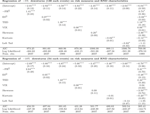
Results forρ=−5% andρ=−10%, with 138 and 54 downturns respectively, are reported in Table 2. As expected from theory, lower FH and higher ES, VIX and TED spread, individually, all indicate a higher probability for a return drawdown. However, in the full regression (12), the VIX looses significance and ES surprisingly changes sign. Hence, only FH and TED spread preserve their predictive characteristics in the joint regression.
The regression results are robust with respect to choice of threshold, ρ, over a wide range of numerical values. Furthermore, stepwise backward model selection (Venables and Ripley, 2002, p. 175) based on the Akaike (1974) information criterion shows that the full model (12) is preferred over all submodels. Finally, a leave-one-out cross-validation (Kohavi et al., 1995) yields a classification rate of 94%.
4.3. The impact of RNDs on risk measures
How do characteristics of the RND shape the various risk measures? To answer that question we regress the risk measures R ∈ R on the (standard-ized) second, third and fourth moment as well as the left tail shape parameter
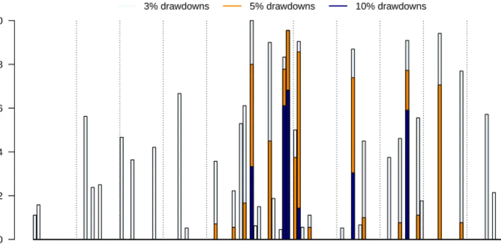
Figure 2: Distribution of return downturns over time.
Fr
action of da
ys in a month with large retur
n dr a wdo wns 0.0 0.2 0.4 0.6 0.8 1.0 2003 2004 2005 2006 2007 2008 2009 2010 2011 2012 2013 3% drawdowns 5% drawdowns 10% drawdowns
Moments when the return decreases by more than a certain value (3, 5 or 10%). Most of the larger drawdowns occur during the Global Financial Crisis (late 2007 to early 2009) as well as the Greek and European sovereign debt crisis in 2010 and 2011, respectively.
of the RNDs:
Rt=a0,t+a1,tRNVt+a2,tSkewt+a3,tKurtt+a4,tLeft Tailt. (13)
Results are presented in Table 3. FH bound captures all variations in the properties of the RND. In particular, a higher RNV and fatter left tail, as well as more negative skewness lead to lower FH.21 By contrast, the other risk measures do not grasp all the RND characteristics. For instance, ES and VIX seem to react mainly to the second moment of the density (RNV), whereas a thinner left tail actually makes them take on higher values. This is particularly surprising in the case of ES, which is formulated specifically to capture tail risks, but a phenomenon that is not an artefact of our esti-mation technique. Moreover, TED spread is significantly explained by the risk-neutral volatility, but not by the tail shape parameter.
21Note, that throughout our data period the RNDs consistently exhibit anegative skew-ness of−1.5±0.9, such that a positive slope coefficient means a reversal to (log-)normality.
Table 2: Regression of return downturns on risk measures.
Regression of −5% downturns (138 such events) on risk measures and RND characteristics
(Intercept) −2.01∗∗∗ −2.92∗∗∗ −3.58∗∗∗ −4.64∗∗∗ −2.35∗∗∗ −2.39∗∗∗ −2.64∗∗∗ −6.04∗∗∗ (0.12) (0.11) (0.14) (0.22) (0.14) (0.11) (0.09) (0.59) −FHQ 1.41∗∗∗ 0.74∗ (0.23) (0.36) ESQ 0.07∗∗∗ −0.08∗∗ (0.02) (0.03) TED 1.30∗∗∗ 1.18∗∗∗ (0.12) (0.18) VIX 0.08∗∗∗ 0.06∗∗∗ (0.01) (0.01) Skewness 0.20∗ −2.36∗∗∗ (0.09) (0.39) Kurtosis −0.02∗∗ −0.14∗∗∗ (0.01) (0.03) Left Tail −0.82∗ −1.11 (0.33) (0.63) AIC 973.25 991.60 860.96 870.30 1006.00 999.11 1006.78 769.06 Log Likelihood -484.62 -493.80 -428.48 -433.15 -501.00 -497.56 -501.39 -376.53 Num. obs. 2037 2037 1989 2037 2037 2037 2037 1989
Regression of −10% downturns (54 such events) on risk measures and RND characteristics
(Intercept) −2.69∗∗∗ −3.80∗∗∗ −4.87∗∗∗ −5.66∗∗∗ −3.47∗∗∗ −3.46∗∗∗ −3.60∗∗∗ −6.70∗∗∗ (0.17) (0.16) (0.24) (0.32) (0.20) (0.16) (0.14) (0.96) −FHQ 2.64∗∗∗ 3.41∗∗∗ (0.49) (0.70) ESQ 0.05∗∗ −0.48∗∗∗ (0.02) (0.13) TED 1.42∗∗∗ 2.44∗∗∗ (0.15) (0.30) VIX 0.08∗∗∗ 0.04 (0.01) (0.03) Skewness 0.09 −3.50∗∗∗ (0.11) (0.74) Kurtosis −0.01 −0.20∗∗∗ (0.01) (0.05) Left Tail −0.14 −1.95 (0.47) (1.15) AIC 458.59 497.84 391.65 431.28 501.77 499.83 502.54 305.41 Log Likelihood -227.30 -246.92 -193.82 -213.64 -248.88 -247.92 -249.27 -144.71 Num. obs. 2037 2037 1989 2037 2037 2037 2037 1989 ∗∗∗p <0.001,∗∗p <0.01,∗p <0.05
This table reports the intercept and slope coefficients of the regression of downturns of ahead-returns until maturity of the underlying option of more than 5% (upper part) or 10% (lower part) on the option-implied Foster-Hart bound FHQ, option-implied expected
shortfall ESQ, the spread between interbank loans and T-Bills TED, and the VIX, as well
as skewness, excess kurtosis and the left tail shape parameter of the risk-neutral density. Standard deviations are given in brackets, significance according to p-values is indicated by stars.
4.4. Time-consistency
Hellmann and Riedel (2015) point out that FH lacks time-consistency, similarly to VaR and ES. Somewhat loosely speaking, they define a risk measure to be time-consistent, if the knowledge of gamble X1
Table 3: Regression of risk measures on RND characteristics. -FHQ ESQ VIX TED (Intercept) −1.08∗∗∗ −2.46∗∗∗ 5.51∗∗∗ 0.05 (0.03) (0.16) (0.23) (0.03) RNV 1.83∗∗∗ 26.78∗∗∗ 79.48∗∗∗ 2.72∗∗∗ (0.07) (0.42) (0.59) (0.09) Skewness −0.19∗∗∗ −0.02 0.30 0.10∗∗∗ (0.02) (0.12) (0.18) (0.03) Kurtosis −0.01∗∗∗ 0.02∗∗ −0.02∗∗ 0.00∗∗ (0.00) (0.01) (0.01) (0.00) Left Tail 0.27∗∗∗ −1.30∗∗∗ −0.79∗ −0.02 (0.04) (0.27) (0.38) (0.06) R2 0.34 0.68 0.91 0.37 Adj. R2 0.34 0.68 0.91 0.37 Num. obs. 2037 2037 2037 1989 RMSE 0.34 2.14 3.05 0.44 ∗∗∗p <0.001,∗∗p <0.01,∗p <0.05
This table reports the intercept and slope coefficients of the regression of various risk measures on characteristics of the density. The risk measures are the option-implied FH bound, the option-implied expected shortfall, the volatility index and the TED spread.
thanX2
t in any state of the world tomorrow should implyXt1 to be considered
riskier than Xt2 already today. Hellmann and Riedel (2015) construct an example showing that, in general, FH is not time-consistent.
Due to the fixed expiration dates of options, our option-implied risk mea-sures also exhibit a naturally dynamic structure, thus raising the issue of time-consistency in the above sense for the special case of risk-neutral densi-ties approaching maturity. Tests thereof, in the sense of Hellmann and Riedel (2015), however, are not possible as the structure of the dynamic gamble is
a priori not known to the representative investor. Instead, we may,
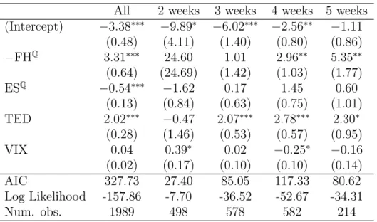
how-ever, get at the issue of predictive time-consistency by comparing how the informativeness of predicting return downturns behaves for the various mea-sures of riskiness depending on the time to maturity. Table 4 summarizes the predictive power of FH, ES, VIX and TED spread when evaluated 2, 3,
4 or 5 weeks before the exercise date of the option. While the slope coeffi-cient of FH is consistently positive, it is significant only 4 and 5 weeks before maturity. Similarly, the TED spread has explanatory power 3 to 5 weeks ahead, whereas the option-implied ES does not show significance at any time window. Surprisingly, the VIX significantly changes sign when derived at dif-ferent times relative to the exercise date. Hence, only FH and TED spread are predictively time-consistent.22
Table 4: Predictive consistency of risk measures.
All 2 weeks 3 weeks 4 weeks 5 weeks (Intercept) −3.38∗∗∗ −9.89∗ −6.02∗∗∗ −2.56∗∗ −1.11 (0.48) (4.11) (1.40) (0.80) (0.86) −FHQ 3.31∗∗∗ 24.60 1.01 2.96∗∗ 5.35∗∗ (0.64) (24.69) (1.42) (1.03) (1.77) ESQ −0.54∗∗∗ −1.62 0.17 1.45 0.60 (0.13) (0.84) (0.63) (0.75) (1.01) TED 2.02∗∗∗ −0.47 2.07∗∗∗ 2.78∗∗∗ 2.30∗ (0.28) (1.46) (0.53) (0.57) (0.95) VIX 0.04 0.39∗ 0.02 −0.25∗ −0.16 (0.02) (0.17) (0.10) (0.10) (0.14) AIC 327.73 27.40 85.05 117.33 80.62 Log Likelihood -157.86 -7.70 -36.52 -52.67 -34.31 Num. obs. 1989 498 578 582 214 ∗∗∗p <0.001,∗∗p <0.01,∗p <0.05
This table reports the intercept and slope coefficients of the regression of downturns of ahead-returns until maturity of the underlying option of more than 10% on the option-implied Foster-Hart bound FHQ, option-implied expected shortfall ESQ, the spread
be-tween interbank loans and T-Bills TED, the VIX and realized volatility by time to ma-turity of the underlying option. Standard deviations are given in brackets, significance according top-values is indicated by stars.
22Recall that it was also FH and TED who preserved their predictive characteristics in the joint estimation of regression (12).
5. Conclusion
The main contribution of this paper has been the translation of the ob-jective risk measure by Foster and Hart (2009) (using Riedel and Hellmann 2015’s and Hellmann and Riedel 2015’s generalizations) to a typical decision context in finance. This was done by extracting the underlying risk-neutral densities from option prices and deriving the corresponding option-implied risk measure. Rather than optimal estimates, we chose an approach which could be described as deriving a conservative bound on these. Our result-ing measure was shown to have additional information compared to standard risk measures. In fact, it outperformed the standard measures including value at risk, expected shortfall, risk-neutral volatility and the volatility index.23 Indeed, not only had our option-implied Foster-Hart measure of riskiness in-teresting macroscopic patterns, in that it indicated rather extreme regime shifts in the dawn of the financial crisis, but also was it shown to be of mi-croscopic interest, in that it turned out a significant predictor of large return downturns. Finally, in future work, we would like to study option-implied Foster-Hart measures in richer investment settings, for example, when in-vestment into more than one asset and/or leverage with hedging is allowed.
23Solely the TED spread (between Libor and Treasury bills), as a measure of credit risk, turned out similarly predictive and consistent, despite the known reliability issues associated with fraudulent Libor setting.
References
A¨ıt-Sahalia, Y. and A. W. Lo (2000). Nonparametric risk management and implied risk aversion. Journal of Econometrics 94(1–2), 9 – 51.
A¨ıt-Sahalia, Y., Y. Wang, and F. Yared (2001). Do option markets correctly price the probabilities of movement of the underlying asset? Journal of
Econometrics 102(1), 67–110.
Akaike, H. (1974). A new look at the statistical model identification.
Auto-matic Control, IEEE Transactions on 19(6), 716–723.
Anand, A., T. Li, T. Kurosaki, and Y. S. Kim (2015). Foster-hart risk and the too-big-to-fail banks: An empirical investigation.
Arrow, K. J. (1971). Essays in the Theory of Risk-Bearing. North Holland, Amsterdam.
Aumann, R. J. and R. Serrano (2008). An economic index of riskiness.
Journal of Political Economy 116(5), 810–836.
Bahra, B. (1996). Probability distributions of future asset prices implied by option prices. Bank of England Quarterly Bulletin 36(3), 299–311.
Bakshi, G., N. Kapadia, and D. Madan (2003). Stock return characteristics, skew laws, and the differential pricing of individual equity options. Review
of Financial Studies 16(1), 101–143.
Bakshi, G. and D. Madan (2000). Spanning and derivative-security valuation.
Journal of Financial Economics 55(2), 205–238.
Bali, T. G., N. Cakici, and F. Chabi-Yo (2011). A generalized measure of riskiness. Management science 57(8), 1406–1423.
Bali, T. G., N. Cakici, and F. Chabi-Yo (2012). Does aggregate riskiness predict future economic downturns? Technical report.
Birru, J. and S. Figlewski (2012). Anatomy of a meltdown: The risk neutral density for the s&p 500 in the fall of 2008. Journal of Financial
Black, F. and M. Scholes (1973). The pricing of options and corporate lia-bilities. The journal of political economy, 637–654.
Bliss, R. R. and N. Panigirtzoglou (2004). Option-implied risk aversion esti-mates. The journal of finance 59(1), 407–446.
Breeden, D. T. and R. H. Litzenberger (1978). Prices of state-contingent claims implicit in option prices. Journal of business, 621–651.
Brown, D. P. and J. C. Jackwerth (2001). The pricing kernel puzzle: Recon-ciling index option data and economic theory.
Chicago Board Options Exchange (2009). The CBOE volatility index – VIX.
White Paper.
Cox, J. C., J. E. Ingersoll Jr, and S. A. Ross (1985). An intertemporal general equilibrium model of asset prices. Econometrica: Journal of the
Econometric Society, 363–384.
Delbaen, F. and W. Schachermayer (1994). A general version of the funda-mental theorem of asset pricing. Mathematische annalen 300(1), 463–520. Embrechts, P., R. Frey, and A. McNeil (2005). Quantitative risk
manage-ment. Princeton Series in Finance, Princeton 10.
Embrechts, P., C. Kl¨uppelberg, and T. Mikosch (1997). Modelling extremal
events: for insurance and finance, Volume 33. Springer.
Epstein, L. G. and S. E. Zin (1991). Substitution, risk aversion, and the tem-poral behavior of consumption and asset returns: An empirical analysis.
Journal of Political Economy, 263–286.
Evstigneev, I. V., T. Hens, and K. R. Schenk-Hopp´e (2006). Evolutionary stable stock markets. Economic Theory 27(2), 449–468.
Fama, E. F. and J. D. MacBeth (1973). Risk, return, and equilibrium: Em-pirical tests. The Journal of Political Economy, 607–636.
Figlewski, S. (2010). Estimating the implied risk neutral density. In T. Boller-slev, J. Russell, and M. Watson (Eds.),Volatility and Time Series
Foster, D. P. and S. Hart (2009). An operational measure of riskiness.Journal
of Political Economy 117(5), 785–814.
Friend, I. and M. E. Blume (1975). The demand for risky assets. The
American Economic Review, 900–922.
Hansen, L. P. and K. J. Singleton (1982). Generalized instrumental vari-ables estimation of nonlinear rational expectations models. Econometrica:
Journal of the Econometric Society, 1269–1286.
Hansen, L. P. and K. J. Singleton (1984). Erratum: Generalized instrumental variable estimation of nonlinear rational expectations models.
Economet-rica 52(1), 267–268.
Hellmann, T. and F. Riedel (2015). A dynamic extension of the fosterhart measure of riskiness. Journal of Mathematical Economics 59, 66 – 70. Jackwerth, J. C. (2004). Option-implied risk-neutral distributions and risk
aversion. Research Foundation of AIMR Charlotteville.
Jondeau, E., S.-H. Poon, and M. Rockinger (2007). Financial modeling under
non-Gaussian distributions. Springer Science & Business Media.
Kelly, J. L. (1956). A new interpretation of information rate. Information
Theory, IRE Transactions on 2(3), 185–189.
Kohavi, R. et al. (1995). A study of cross-validation and bootstrap for accu-racy estimation and model selection. In Ijcai, Volume 14, pp. 1137–1145. Kostakis, A., N. Panigirtzoglou, and G. Skiadopoulos (2011). Market timing
with option-implied distributions: A forward-looking approach.
Manage-ment Science 57(7), 1231–1249.
Leiss, M., H. H. Nax, and D. Sornette (2015). Super-exponential growth expectations and the global financial crisis.Journal of Economic Dynamics
and Control 55, 1 – 13.
Melick, W. R. and C. P. Thomas (1997). Recovering an asset’s implied pdf from option prices: an application to crude oil during the gulf crisis.
Normandin, M. and P. St-Amour (1998). Substitution, risk aversion, taste shocks and equity premia. Journal of Applied Econometrics 13(3), 265– 281.
Panigirtzoglou, N. and G. Skiadopoulos (2004). A new approach to modeling the dynamics of implied distributions: Theory and evidence from the S&P 500 options. Journal of Banking & Finance 28(7), 1499–1520.
Riedel, F. and T. Hellmann (2015). The foster-hart measure of riskiness for general gambles. Theoretical Economics 10(1), 1–9.
Rubinstein, M. (1994). Implied binomial trees.The Journal of Finance 49(3), 771–818.
Samuelson, P. A. (1979). Why we should not make mean log of wealth big though years to act are long.Journal of Banking & Finance 3(4), 305–307. Shimko, D. C., N. Tejima, and D. R. Van Deventer (1993). The pricing of risky debt when interest rates are stochastic. The Journal of Fixed
Income 3(2), 58–65.
S¨oderlind, P. and L. Svensson (1997). New techniques to extract mar-ket expectations from financial instruments. Journal of Monetary
Eco-nomics 40(2), 383–429.
Venables, W. and B. Ripley (2002). Modern Applied Statistics with S. Statis-tics and Computing. Springer.
Whitworth, W. (1870). Choice And Chance. Deighton, Bell and Co, Cam-bridge.
Xing, Y., X. Zhang, and R. Zhao (2010, 6). What does the individual option volatility smirk tell us about future equity returns? Journal of Financial