Geometric Particle Swarm Optimization for Multi-objective Optimization Using Decomposition

(1)

Geometric Particle Swarm Optimization for Multi-objective

Optimization Using Decomposition

Saúl Zapotecas-Martínez

Shinshu University Faculty of Engineering 4-17-1 Wakasato, Nagano, 380-8553, Japan

Alberto Moraglio

University of Exeter Department of Computer Science Exeter EX4 4QF, UK

Hernán E. Aguirre

Kiyoshi Tanaka

ABSTRACT

Multi-objective evolutionary algorithms (MOEAs) based on decomposition are aggregation-based algorithms which trans-form a multi-objective optimization problem (MOP) into several single-objective subproblems. Being effective, effi-cient, and easy to implement, Particle Swarm Optimization (PSO) has become one of the most popular single-objective optimizers for continuous problems, and recently it has been successfully extended to the multi-objective domain. How-ever, no investigation on the application of PSO within a multi-objective decomposition framework exists in the con-text of combinatorial optimization. This is precisely the focus of the paper. More specifically, we study the incorpo-ration of Geometric Particle Swarm Optimization (GPSO), a discrete generalization of PSO that has proven successful on a number of single-objective combinatorial problems, into a decomposition approach. We conduct experiments onmany -objective 1/0 knapsack problems i.e. problems with more than three objectives functions, substantially harder than multi-objective problems with fewer objectives. The results indicate that the proposed multi-objective GPSO based on decomposition is able to outperform two version of the well-know MOEA based on decomposition (MOEA/D) and the most recent version of the non-dominated sorting genetic al-gorithm (NSGA-III), which are state-of-the-art multi-objec-tive evolutionary approaches based on decomposition.

Keywords

Multi-objective Combinatorial Optimization;

Decomposition-Permission to make digital or hard copies of all or part of this work for personal or classroom use is granted without fee provided that copies are not made or distributed for profit or commercial advantage and that copies bear this notice and the full cita-tion on the first page. Copyrights for components of this work owned by others than ACM must be honored. Abstracting with credit is permitted. To copy otherwise, or re-publish, to post on servers or to redistribute to lists, requires prior specific permission and/or a fee. Request permissions from [email protected].

GECCO ’16, July 20-24, 2016, Denver, CO, USA

c

2016 ACM. ISBN 978-1-4503-4206-3/16/07. . . $15.00 DOI:http://dx.doi.org/10.1145/2908812.2908880

based MOEAs; Particle Swarm Optimization.

1. INTRODUCTION

Particle swarm optimization (PSO) [13] is a bio-inspired metaheuristic for continuous optimization problems, which has been applied very successfully to many engineering and scientific problems. This has motivated researchers to ex-tend it to multi-objective optimization problems (MOPs). In the last decade, several multi-objective particle swarm optimizers (MOPSOs) have been developed (see [26] for a good survey on this topic). Most of these approaches use a set of best non-dominated solutions to steer the search, rather than a single global optimum as in the traditional PSO, along with an additional mechanism to maintain pop-ulation diversity during the search. These approaches be-came very popular in the early days of MOPSOs.

The dominance resistance phenomenon [24], which is com-monly observed in problems with more than 3 objectives (known asmany-objective problems), hinders performances of MOPSOs using Pareto dominance relation by making se-lection ineffective. Researchers have then focused on de-veloping alternative selection mechanisms to deal with this drawback, such as for example methods based on indica-tors [6, 15]. Recently, researchers working on MOEAs have adopted the idea of decomposing a MOP into several op-timization subproblems. This approach has become one of the most useful strategies to deal with MOPs, especially for many-objective problems, see for instance [31, 9]. In this approach, a set of approximate solutions to the Pareto op-timal front is achieved by minimizing each single-objective subproblem, rather than using Pareto optimality or alter-native selection mechanisms. This trend has also led to a new generation of multi-objective particle swarm optimizers based on decomposition studied by several authors, see for example [23, 21, 33]. To date, these approaches have focused on continuous and unconstrained problems, leaving the dis-crete case as an open field to be explored. This is precisely the focus of the work reported herein.

(2)

introduced to date, the majority of these operating on bi-nary strings, see e.g. [14, 1, 18, 22]. Extensions of PSO to more complex combinatorial search spaces, such as per-mutations or TSP tours, are rarer but do exist, see e.g. [7]. The difficulty here lays in defining meaningful notions of motion, direction, and velocity in such spaces. Geometric particle swarm optimization (GPSO) [19] is a generalization of traditional particle swarm optimization to general metric spaces. These notions and the PSO algorithm dynamics are defined in this general abstract setting. Specific instantia-tions of GPSO can then be formally derived by using spe-cific distances and associated solution representations in the general definition of GPSO. This approach has the advan-tage that PSO for specific representations can be derived in a principled way, rather than reinvented and adapted ad-hoc to each new representation. Representation-specific GPSO have been derived for binary strings [19], permuta-tions and applied to solving Sudoku [20], and tree structures and used as an alternative search strategy for genetic pro-gramming [29]. The binary GPSO has been successfully adopted in several applications, e.g. [2, 3, 11, 28, 25].

In this paper, we introduce a new multi-objective particle swarm optimizer for combinatorial problems. The proposed approach extends the binary GPSO to work with MOPs adopting the decomposition approach. The study presented here indicates that the proposed approach is efficient and produces a good approximation to the Pareto front on multi-objective knapsack problems with a number of multi-objectives ranging from two to ten. It is also found to be significantly better than the well-known multi-objective evolutionary al-gorithm based on decomposition (MOEA/D) [34] and than the most recent version of the non-dominated sorting genetic algorithm (NSGA-III) [9].

2. BASIC CONCEPTS

2.1 Preliminaries of Multi-objective

Optimiza-tion

Assuming maximization, a general multi-objective opti-mization problem (MOP) can be stated as:

maximize: F(x)

s.t. gi(x)≤0, i= 1, . . . , p

hj(x) = 0, j= 1, . . . , q

x∈X

(1)

wherex= (x1, . . . , xn)⊺ is anndimensional vector of

deci-sion variables. The vectorF= (f1(x), . . . , fM(x))⊺consists

ofM objective functionsfj’s to be maximized. gi(x)≤0

andhj(x) = 0 represent thepinequality constraints and the

qequality constraints, respectively. The set of solutions that satisfy the constraints of problem (1) defines the feasible re-gion Ω ⊂ X. When problem (1) is continuous X = Rn_. In the case of pseudo-boolean combinatorial problems the search space isX ={0,1}n_.

The following definitions introduce the concept of opti-mality of interest in this paper (see [17]).

Definition _1. _Let x,y ∈ Ω, we say that x dominates

y (denoted by x ≻y) if and only if: 1) fi(x)≥ fi(y) for all i ∈ {1, . . . , M} and 2) fj(x) > fj(y) for at least one

j∈ {1, . . . , M}.

Definition 2. Let x⋆ _∈ _Ω_{, we say that} _x⋆ _{is a} _Pareto

optimal solution, if there is no other solution y ∈ Ω such thaty≻x⋆.

Definition 3. ThePareto optimal setP Sis defined by: P S={x∈Ω|x is a Pareto optimal solution}and its image P F ={F(x)|x∈P S}) is calledPareto frontP F.

In multi-objective optimization problems, we are typically interested in finding a finite number of elements from the Pareto set, while maintaining a proper representation of the Pareto front.

2.2 Decomposition of a Multi-objective

Opti-mization Problem

It is well-known [17] that a Pareto optimal solution to the problem (1) is an optimal solution of a scalar optimiza-tion problem in which the objective is an aggregaoptimiza-tion of all the objective functions fi’s. Many scalar approaches

have been proposed to aggregate the objectives of a MOP. Among them, the Tchebycheff approach [5] is one of the most used methods, and it is the one adopted in this study. Other scalarization approaches could also be easily used, see e.g., [10, 17].

Tchebycheff approach. This approach transforms the vec-tor of function valuesFinto a scalar maximization problem which is of the form:

minimize gtch₍

x|λ,z) = max

1≤j≤M{λj|zj−fj(x)|}

s.t. x∈Ω (2)

where Ω is the feasible region, z= (z1, . . . , zk)⊺ is the

ref-erence point such that zj = max{fj(x)|x ∈ Ω} for each

i= 1, . . . , M, andλ= (λ1, . . . , λM)⊺is a weight vector, i.e.,

λj≥0 for allj= 1, . . . , M andPM_j=1λj= 1.

For each Pareto optimal pointx⋆, there exists a weight vectorλsuch thatx⋆_{is the optimum solution of equation (2)}

and each optimal solution of equation (2) is a Pareto optimal solution of equation (1). An appropriate representation of the Pareto front could be reached by solving different scalar-izing problems. Such problems can be defined by a set of well-distributed weight vectors, which establish the search direction in the optimization process.

Therefore, a proper approximation to the Pareto front can be reached by minimizing a set of scalarizing functions de-fined by a well-distributed set of weights vectors. This is the main idea behind mathematical programming methods for multi-objective problems and current multi-objective evo-lutionary approaches based on decomposition, e.g. [34, 23, 16].

2.3 Geometric Particle Swarm Optimization

The generalization of the standard PSO algorithm for con-tinuous spaces to general metric spaces is based on the fol-lowing idea (see [19] for more details and the mathematical derivation). The only elements of the standard PSO algo-rithm that depend on the underlying representation are the velocity update and position update equations which require velocities and positions to be real vectors. The velocity up-date equation can be factored out and equivalently restated in terms of current and past positions of each particle. In absence of inertia, the new position of a particle can be written as a convex combination of its current position, its

(3)

Figure 1: The convex combination operator moves the par-ticle based on its current position, position of its personal best and position of the global best.

personal best position, and the position of the global best (see figure 1).

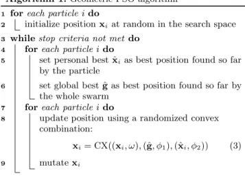
As the notion of convex combination is well-defined in gen-eral metric spaces, the PSO algorithm can then be readily generalized to metric spaces. The generic Geometric PSO algorithm is illustrated in Algorithm 1. This differs from the standard PSO in that: (i) there is no explicit velocity up-date equation (but particles have velocities as they move); (ii) the equation of the position update is a (randomized) convex combination as outlined above, with weightsω,φ1, andφ2, which are are non-negative and add up to one; (iii) the new position undergoes to mutation to partly compen-sate for the lack of inertia.

The specific PSO for the space of binary strings1

endowed with Hamming distance can be obtained by formally deriv-ing an explicit definition of randomized convex combination for this space in terms of manipulation of the underlying rep-resentation. This operator then specifies operationally how to obtain an ’offspring’ binary string which corresponds to the convex combination of ‘parent’ binary strings. In [19], this operator was shown to be a straightforward general-ization of mask-based crossover for two parents to a three-parental recombination, in which the probability of inherit-ing a bit at each position from a parent strinherit-ing is given by its weight in the convex combination. The mutation employed in binary GPSO is standard bit-wise mutation.

3. MULTI-OBJECTIVE GPSO BASED ON

DECOMPOSITION

Our proposed multi-objective GPSO based on decomposi-tion (MO-GPSO/D) decomposes a MOP into several single-objective subproblems by using an aggregation function and a weight vector, as in MOEA/D [34]. However, the proposed approach does not follow the principles of MOEA/D. The main differences between MOEA/D and MO-GPSO/D are the recombination and replacement strategies.

Recombination strategy. MOEA/D defines a neighborhood in order to select random solutions to be recombined. For bi-nary combinatorial problems, MOEA/D adopts traditional operators taken from genetic algorithms (specifically, one-point crossover, and bit-wise mutation), in order to gener-1_{A Python implementation of this algorithm is available at} https://github.com/amoraglio/.

Algorithm 1:Geometric PSO algorithm

1 foreach particleido

2 initialize positionxiat random in the search space 3 whilestop criteria not met do

5 set personal best ˆxias best position found so far

by the particle

6 set global best ˆgas best position found so far by

the whole swarm

8 update position using a randomized convex

combination:

xi= CX((xi, ω),(ˆg, φ1),(ˆxi, φ2)) (3)

9 mutatexi

ate candidate solutions, see [34]. This strategy works well in continuous problems. However, in the case of combinato-rial problems (where the fitness landscape is unknown) the regulatory property of continuous MOPs (the idea behind of MOEA/D [34]) does not claim that an optimal solution of a subproblem with weightλ1, is close to other optimal solution of other subproblem with weight λ2

, for||λ1 −λ2

||< ǫ(for anǫsmall enough), i.e. neighboring subproblems. Therefore we hypothesize that MO-GPSO/D could work better than MOEA/D if the recombination of solutions is not restricted into a single neighborhood as in MOEA/D. MO-GPSO/D uses the geometric version of PSO to create new solutions by using thepersonal best(the best position of the particle to theith subproblem) and theglobal bestsolution (solution found from all the swarm which achieves the best value for theith subproblem along the search).

Replacement strategy. MOEA/D replaces all solutions in the neighborhood which are improved by the new candidate solution. This mechanism works well for MOPs having rel-atively easy Pareto sets [16]. However, for more complex problems (see for example [35]), this strategy becomes in-efficient and sometimes impractical. In fact, this strategy can misplace diversity in the population specially in multi-modal problems or problems with rugged landscapes. This drawback was treated in [16] where a dynamic neighbor-hood selection and a maximum number replacements were implemented, arising in a new version of MOEA/D namely MOEA/D-DE. In MO-GPSO/D, the replacement of global best solutions is carried out in different way. We do not re-place all the improved solutions with the new one. Instead of this, the new solution is in competition with the current best solutions and from them, the new set of global best solutions is defined. Therefore, we speculate that this mechanism could maintain more diversity in the population, which is especially important in multi-objective optimization, while at the same time, GPSO steers the search towards promising regions employing the best solutions found along the search.

The pseudocode of the proposed MO-GPSO/D is pre-sented in Algorithm 2. To follow a decomposition of a MOP, a well-distributed set of weighted vectors Λ ={λ1, . . . , λN}

(4)

com-plete algorithm works as follows.

At the beginning of the algorithm, the set of the positions of theNparticlesP ={p1, . . . ,pN}is randomly initialized. In MO-GPSO/D, theith particle is set to optimize one of the subproblems defined by the weighted vectorλi. To this end, in the main cycle, each particle ‘flies’ towards a better position for its single particular subproblem, i.e., the one with objective functiongtch₍

pi|λi,z⋆) for theith particle. The best personal position is initialized with the initial position of the particle, i.e., ˆpi ₌_pi_{. On the other hand,}

the set ofglobal bestpositionsGbest is stated by the initial

positionsP, i.e. Gbest=P.

The position of each particle is updated by using the recorded personal best and the global best of each particle. Then the bitwise mutation is employed as turbulence oper-ator on each particle. Once a new position is computed, the reference point needs to be updated (line 10 in Algorithm 2). Then, the personal best ˆpi is updated if the new position improves the previous position (line 12 in Algorithm 2).

Throughout the search, the set of global bests (denoted by Gbest={ˆg1, . . . ,ˆgN}) shall contain the solutions that

opti-mize each separate subproblem. This set of solutions is then updated when a new candidate solution is generated (line 17 in Algorithm 2). Thus, the notion of elitism used in evolu-tionary multi-objective optimization is implicitly employed in our proposed approach.

The proposed approach tries to optimize a set of subprob-lems whose final solutions should be very close to the Pareto optimal set. We expect that all solutions inGbestare equally

good i.e., that all the subproblems will be approximately sat-isfactorily solved, as the same search procedure and search effort is applied to all of them. Therefore, at the end of the search this set of solutions is considered as the final approx-imation to the Pareto optimal set.

4. EXPERIMENTAL DESIGN

4.1 Multi-Objective 0/1 Knapsack Problem

In order to test the performance of the proposed MO-GPSO/D, the knapsack problem, one of the most stud-ied NP-hard problems from combinatorial optimization, is adopted in a multi-objective optimization context.

Given a collection of nitems and a set ofM knapsacks, the multi-objective 0/1 knapsack problem (MO-KNP) seeks a subset of items subject to capacity constraints based on a weight functionvectorw: [0,1]n_→_NM_{, while maximizing}

aprofit functionvectorp: [0,1]n_→_NM_{. Formally it can be}

stated as: maximize: fj(x) =Pn_i=1pji·xi j∈ {1, . . . , M} s.t. Pn i=1wji·xi6cj j∈ {1, . . . , M} xi∈ {0,1} i∈ {1, . . . , n} (4)

wherepji∈Nis the profit of item ion knapsackj,wji∈N

is the weight of item i on knapsack j, and cj ∈ N is the

capacity of knapsackj.

We consider the conventional instances proposed in [37], with random uncorrelated profit and weight integer values taken uniformly from [10,100]. The capacity is set to half of the total weight of a knapsack for each objective function, i.e. cj = 12

Pn

i=1wji for j= 1, . . . , M. As a result, about

50% of the items are expected to be in the Pareto optimal front.

Algorithm 2:General Framework of MO-GPSO/D Input:

N: the number of subproblems to be decomposed; Λ: a well-distributed set of weight vectors{λ1_{, . . . , λ}N_}_; Output:

P: the final approximation to the Pareto set. 1 z= (−∞, . . . ,−∞)⊺;

2 Generate a random set of solutionsP={p1, . . . ,pN}in Ω; 3 G_best=P;

4 fori= 1, . . . , N do 5 ˆpi=pi;

6 z_j= max(z_j, f_j(pi)); // j∈ {1, . . . , M} 7 whilestopping criterion is not satisfieddo

8 for pi∈P do

9 Update Position: Update position using a randomized convex combination:

pi= CX((pi, ω),(ˆgi, φ1),(ˆpi, φ2)) 10 Turbulence: Apply turbulence operator to the new

particle:

pi=mutation(pi) 11 Update z: Update the reference pointz:

zj= max(zj, fj(pi)); // j∈ {1, . . . , M}

12 Update Personal Best:

13 Ifgtch(pi|λi,z)≥gtch(ˆpi|λi,z) then ˆpi=pi;

14 Update Global Bests:

15 Q=G_best∪ {pi}; 16 forj∈ {1, . . . , N}do 17 ˆq= arg max q∈Q gtch (q|λj_,_z_); 18 ˆ_gj= ˆ_q; 19 Q=Q\ {q}ˆ ; 20 returnG_best={gˆ1, . . . ,gˆN};

Random problem instances of 128 items are investigated for each objective space dimension. We consider instances with 2, 3, 5, 8, and 10 objectives2

.

In order to satisfy the constraints of the problem, we adopt a standard decoding procedure which guarantees the fea-sibility of solutions as proposed in [37]. This procedure removes items sorted in increasing order of the maximum profit/weigh ratio over all knapsacks one at a time, until all constraints are satisfied.

4.2 Experimental Setup

We compare experimentally MO-GPSO/D with three state-of-the-art MOEAs based on decomposition: the original MO-EA/D [34], its new variant MOMO-EA/D-DE [16] adapted to binary spaces (as explained below) and NSGA-III [9].

The method MOEA/D-DE extends MOEA/D as follows: it uses dynamic selection of the neighborhood with a given probabilityδ, and a fixed maximum number of replacements nr in the neighborhood. Furthermore, MOEA/D-DE uses

Differential Evolution (DE) operator as reproduction mech-anism, which is however defined for continuous spaces. To adapt this algorithm to binary string spaces, the DE op-erator is replaced with standard crossover and mutation operators for binary strings, as in the original version of 2

The set of instances adopted in our comparative study are available at http://computacion.cs.cinvestav.mx/ ˜zapoteca/MO-KNP/

(5)

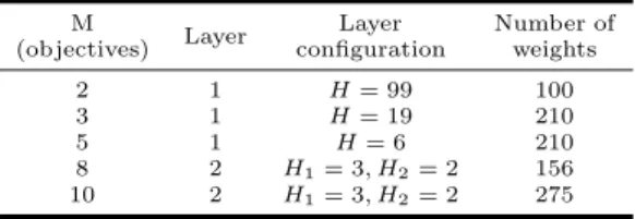
Table 1: Configuration for the two-layered simplex-lattice design

M

Layer Layer Number of

(objectives) configuration weights

2 1 H= 99 100

3 1 H= 19 210

5 1 H= 6 210

8 2 H1= 3, H2= 2 156

10 2 H1= 3, H2= 2 275

MOEA/D, see [34]. We adopted this variant in order to test the performances of MOEA/D with dynamic selection and the limit on the number of replacements. In the rest of the paper, we refer to this variant as MOEA/D*.

For fairness, the set of weight vectors for all the algo-rithms in the comparison was the same, and it was gener-ated using the Simplex-lattice design [27], as follows. The settings ofN (number of weights and population size) and Λ ={λ1

, . . . , λN} are controlled by a parameterH. More precisely, λ1, . . . , λN are weight vectors whose component scalar weightsλi

j(i= 1, . . . , N andj= 1, . . . , M) take

val-ues in 0 H,

1 H, . . . ,

H

H . Therefore, the number of all

pos-sible choice of vectors in Λ is given by N = C_HM+−M1−1, whereM is the number of objective functions. Since, this number increases binomially with the number of objectives, this methodology becomes quickly impractical when we have more than a handful of objectives. A strategy to deal with high dimensional spaces is proposed in [9], known as the two-layered simplex-lattice design. This strategy uses the simplex-lattice design to generate an outside layer and an inside layer in the weights set. Fig. 2 illustrates the two-layered simplex-lattice design inR3

when usingH1 = 2 for the outside layer and H2 = 1 for the inside layer. In this study, we compare the decomposition-based approaches by using the weights given by the two-layered simplex-lattice design for problems with more than 5 objectives, otherwise a single layer is employed. The complete configuration ofH values for different dimensions of the two-layered simplex-lattice design is shown in Table 1.

In our comparison, MOEA/D, MOEA/D*, and NSGA-III use the same reproduction operators, one-point crossover and bit-wise mutation, as in the original version of MO-EA/D [34]. MO-GPSO/D uses also bit-wise mutation as turbulence operator.

Table 2 presents the parameter settings used in our exper-imental study. The parameters for the adopted algorithms

Figure 2: Illustration of the two-layered simplex-lattice de-sign. The outside layer is stated byH1 = 2 (generating six weights vectors), while the inside layer is set by H2 = 1 (generating three weights vectors)

Table 2: Parameters for MO-GPSO/D, MOEA/D, MOEA/D*, and NSGA-III

Parameter MO-GPSO/D MOEA/D MOEA/D* NSGA-III

T — 20 20 — δ — — 0.9 — nr — —- 2 — Pc — 1 1 1 Pm 1/n 1/n 1/n 1/n ω 1/3 —- – — φ1 1/3 —- – — φ2 1/3 —- – —

are set as suggested by their respective authors. T is the neighborhood size for MOEA/D and MOEA/D*,δ andnr

are the probability of selecting a determined neighborhood and the maximum number of replacements in the neighbor-hood (for MOEA/D*). PcandPmare the crossover rate and

mutation rate. ω, φ1andφ2are the weights used in GPSO. Finally, the search for all the evolutionary approaches was restricted to perform 2,000 generations.

4.3 Performance Assessment

In this section, we outline the performance measures used in our comparison, and the method employed to define the reference setR.

4.3.1 Performance measures

Set Two Coverage (C). Set Two Coverage(C) was pro-posed by Zitzler et al. [36], and it compares a set of non-dominated solutionsAwith respect to another setB, using Pareto dominance. This performance measure is defined as:

C(A, B) = |{b∈B|∃a∈A:ab}|

|B| (5)

If all points inA dominate or are equal to all points inB, this implies that C(A, B) = 1. Otherwise, if no point of A dominates some point in B then C(A, B) = 0. When

C(A, B) = 1 andC(B, A) = 0 then, we say thatAis better than B. Since the Pareto dominance relation is not sym-metric (i.e. not alwaysC(A, B) =C(B, A) is held), we need to calculate bothC(A, B) andC(B, A).

Inverted Generational Distance (IGD). The Inverted Generational Distance (IGD) [8] indicates how far a given Pareto front approximation is from a reference set. LetR be a proper representation of the Pareto optimal front, the

IGDfor a set of approximated solutionsP is calculated as:

IGD(P) = 1 |R|

P

v∈Rd(v, P) (6)

where d(v, P) is a minimum distance between v and any point inP and|R|is the cardinality ofR. TheIGDmetric can measure both convergence and diversity when the ref-erence set R is a proper representation of the true Pareto front. A value of zero in this performance measure, indicates that all the solutions obtained by the algorithm are on the true Pareto front, it is the best possible value.

4.3.2 Reference set definition

From problem in Equation (2) and replacing the objective function and constraints by the multi-objective 1/0

(6)

knap-sack problem (Equation (4)), we have: minimize: gtch(x|λ,z) = max 1≤j≤M{λj|zj−fj(x)|} = max 1≤j≤M λj zj− _n P i=1 pji·xi s.t. n P i=1 wjixi ≤cj, j= 1, . . . , M (7) by introducing the relaxed formulation (i.e. allowing real numbers such that 0≤xi ≤1), the above problem can be

rewritten in its linear form as [12]: minimize: α s.t. λj zj−Pni=1pjixi ≤α Pn i=1wjixi ≤cj, 0≤xi≤1, i= 1, . . . , n for allj= 1, . . . , M (8)

where z = (z1, . . . , zM)⊺ is the reference point and λ =

(λ1, . . . , λM)⊺is a weight vector satisfyingPMj=1zj= 1 and

λi≥0.

For each instance, we generated the reference setR solv-ing a large number of relaxed linear problems (Equation (8)) defined by different weight vectors. Since the reference set Rshould contain a large enough number of points to ensure a good measurement of theIGDmetric, we should generate a finite but well-distributed set of weight vectors. Simplex lattice method becomes impractical to define a specific num-ber of weight vectors in high-dimensional spaces, therefore, we used the methodology presented in [32] and generated 200×M weight vectors (whereM denotes the number of objectives). All the solutions for different weight vectors of problem (8), give the pointsF(x)’s (in the objective space). Therefore, for a specific instance, the obtained points con-stitute the reference setR.3

For each instance, the reference pointzwas found by indi-vidual optimization of each separate objective in the relaxed multi-objective 0/1 knapsack problem. Note that all feasible solutions of the multi-objective 0/1 knapsack problem, are also feasible solutions of the relaxed problem. Therefore, the optimum values of each objective on the relaxed problem is not worse than the optimum value of this objective on the original problem [12]4

.

5. DISCUSSION OF RESULTS

We compared experimentally our proposed MO-GPSO/D with MOEA/D, MOEA/D*, and NSGA-III on knapsack problems with 2, 3, 5, 8, and 10 objectives.

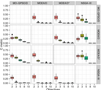
Figure 3 shows the results of the evaluation with the per-formance measureC. In order to illustrate the general per-formance of the algorithms in comparison, simple box plots are shown. The thick line represents the median value, the upper and lower ends of the box are the upper and lower quartiles, and the ends of the vertical line are minimum and maximum values. We computed theCperformance measure by comparing pairs of algorithms (i.e.,C(A, B) andC(B, A)). These values were obtained as average values of the compar-3

The weight vectors and reference set for each in-stance are available at http://computacion.cs.cinvestav.mx/ ˜zapoteca/MO-KNP/

4_{In order to solve the linear optimization problem, we use} the Python SciPy library by employing the Simplex method.

MO−GPSO/D MOEA/D MOEA/D* NSGA−III

0.00 0.25 0.50 0.75 1.00 0.00 0.25 0.50 0.75 1.00 0.00 0.25 0.50 0.75 1.00 0.00 0.25 0.50 0.75 1.00 MO−GPSO/D MOEA/D MOEA/D* NSGA−III 2 3 5 8 10 2 3 5 8 10 2 3 5 8 10 2 3 5 8 10 Objectives C metr ic Instance KNP−2 KNP−3 KNP−5 KNP−8 KNP−10

Figure 3: Results of the comparison with C(A, B) perfor-mance measure. Each chart contains five box plots repre-senting the distribution ofCvalues for a certain ordered pair of algorithms. Scale is zero at the bottom and one at the top for each chart. Chart in row of algorithm A and column of algorithm B presents values of convergence of approxima-tions generated B by approximaapproxima-tions generated by A.

isons of all independent runs of algorithmA with all inde-pendent runs of algorithm B.

In these charts, we show the ratio of solutions produced by MO-GPSO/D that dominate the solutions produced by MOEA/D, MOEA/D* and NSGA-III, respectively. This Figure must be read as C(A, B), where A denotes the al-gorithm in row, andB the algorithm in column. As we can see, the algorithms have a similar performance in the two-objective problem. The same behavior can be observed for problems with three objectives. However, when the num-ber of objectives is increased, the ratio of solutions domi-nated by any algorithm decreases. It does not mean that the algorithms decrease their performance. When the val-ues ofC(A, B) andC(B, A) are almost the same, and they are small, it means that both algorithms are competitive in terms of Pareto relation (and this is the behavior of MOEAs with 5, 8, and 10 objectives). However, in terms of approxi-mating the complete Pareto front, this metric could be mis-understood. It can be the case that algorithm A and B produce a small value for theCmetric. However, solutions produced by algorithmAcan draw a suitable representation of the Pareto front while solutions produced by algorithmB can be biased in a specific part of the Pareto front. In order to investigate precisely this behavior, we use theIGD per-formance measure which assesses the distance of solutions produced by an algorithm to the reference Pareto front.

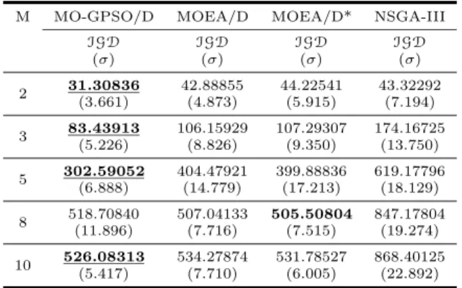
Table 3 shows the results obtained by the algorithms in the comparison with respect to the second performance mea-sure, IGD. In each cell, the number on the top is the av-erage indicator-value (lower is better), and the number

(7)

be-Table 3: Table of results achieved by MO-GPSO/D, MOEA/D, MOEA/D*, and NSGA-III for the MO-KNP with 2, 3, 5, 8, and 10 objectives in the IGD performance measure.

M MO-GPSO/D MOEA/D MOEA/D* NSGA-III

IGD IGD IGD IGD

(σ) (σ) (σ) (σ) 2 31.30836 42.88855 44.22541 43.32292 (3.661) (4.873) (5.915) (7.194) 3 83.43913 106.15929 107.29307 174.16725 (5.226) (8.826) (9.350) (13.750) 5 302.59052 404.47921 399.88836 619.17796 (6.888) (14.779) (17.213) (18.129) 8 518.70840 507.04133 505.50804 847.17804 (11.896) (7.716) (7.515) (19.274) 10 526.08313 534.27874 531.78527 868.40125 (5.417) (7.710) (6.005) (22.892)

low it in brackets is the standard deviation. Best values for each problem instance are reported in bold. Underlined values correspond to algorithms that are not statistically outperformed by any other algorithm for the instance under consideration (using a Mann-Whitney-Wilcoxon [30] non-parametric statistical test with a p-value of 0.05 with Bon-ferroni correction [4]).

As we can see from Table 3, the performance of the MO-EA/D, MOEA/D* and NSGA-III are very similar for in-stances with two objectives, while MO-GPSO/D is signifi-cantly better. The performance of MO-GPSO/D is (statis-tically significantly) better than all the other algorithms in the comparison, except on the problem with 8 objectives, on which MOEA/D* is better than MO-GPSO/D, but the dif-ferences between their performance is not statistically signif-icant. This analysis suggests that the way we couple GPSO into a multi-objective decomposition framework is a good strategy for the type of problems under study. It is also remarkable that the performance of NSGA-III decreases as the number of objective increases. The main reason for this is that NSGA-III relies on a suitable construction of the hy-perplane, which is essential for a correct fitness assignment to solutions. Such hyperplane is defined by finding the best solutions in the population that minimizes the achievement scalarization function (ASF) [9] with the canonical basis (in RM_{). However, in discrete problems, optimal solutions to} the ASF with the specific weight vector cannot be found (it could be not exist). This could generate a bad definition of such hyperplane and lead to a wrong ranking of solutions.

Finally, Figure 4 reports the complete convergence plots for the algorithms in the comparison. This plot also cor-roborates the good performance achieved by MO-GPSO/D in the test instances (specially in problems with 2, 3, and 5 objectives), as the plot of MO-GPSO/D is lower than the plots of the other algorithms.

6. CONCLUSIONS AND FUTURE WORK

We have proposed a new multi-objective particle swarm optimizer using the geometric particle swarm optimization algorithm within a multi-objective framework based on de-composition. The proposed approach was designed to deal with combinatorial MOPs with both low and high dimen-sionality (in terms of the number of objectives).

2 objectives 3 objectives 5 objectives

8 objectives 10 objectives 100 1000 100 1000 ₁₀₀₀ 1000 1000 0 500 1000 1500 2000 0 500 1000 1500 2000 Generations IGD metr ic MOEA MO−GPSO/D MOEA/D MOEA/D* NSGA−III IGD Convergence plot

Figure 4: Convergence plots (in log scale) for IGD perfor-mance measure on the MO-KNPs having 2, 3, 5, 8, and 10 objective functions, respectively.

The proposed approach follows the decomposition approach in the sense that it optimizes a set of scalarizing functions but it does not follow other principles of MOEA/D, i.e. neighborhoods, dynamic selection or limit on maximum num-ber replacements.

Experimental results indicate that our proposed approach (i.e. MO-GPSO/D) outperforms significantly three state-of-the-art MOEAs based on decomposition, namely MOEA/D, MOEA/D*, and NSGA-III, on the test problems adopted.

In future work, we will test MO-GPSO/D on more com-plex and on a greater variety of problems to identify strengths and weakness of this algorithm. We will also analyze the scalability of MO-GPSO/D with MOPs with large scale i.e., large number of bits. Finally, we will consider improvements to the proposed approach by introducing local search mech-anism during the search process.

7. REFERENCES

[1] D. Agrafiotis and W. Cede ˜A´so. Feature selection for structure-activity correlation using binary particle swarms.Journal of Medicinal Chemistry,

45(5):1098–1107, 2002.

[2] E. Alba, J. Garc´ıa-Nieto, L. Jourdan, and E.-G. Talbi. Gene selection in cancer classification using pso/svm and ga/svm hybrid algorithms. InEvolutionary Computation, 2007. CEC 2007. IEEE Congress on, pages 284–290. IEEE, 2007.

[3] E. Alba, J. Garc´ıa-Nieto, J. Taheri, and A. Zomaya. New research in nature inspired algorithms for mobility management in gsm networks. In

Applications of Evolutionary Computing, pages 1–10. Springer, 2008.

[4] C. E. Bonferroni. Teoria statistica delle classi e calcolo delle probabilita.Pubblicazioni del R Istituto Superiore di Scienze Economiche e Commerciali di Firenze, 8:3–62, 1936.

[5] V. J. Bowman Jr. On the relationship of the tchebycheff norm and the efficient frontier of multiple-criteria objectives. InLecture Notes in Economics and Mathematical System, volume 130, pages 76–86. 1976.

[6] I. Chaman Garcia, C. Coello Coello, and A. Arias-Montano. Mopsohv: A new

(8)

optimizer. InCEC’2014, pages 266–273, July 2014. [7] M. Clerc. Discrete particle swarm optimization,

illustrated by the traveling salesman problem. InNew Optimization Techniques in Engineering, pages 219–239. Springer, 2004.

[8] C. A. Coello Coello, G. B. Lamont, and D. A. Van Veldhuizen.Evolutionary Algorithms for Solving Multi-Objective Problems. Springer, New York, second edition, September 2007. ISBN 978-0-387-33254-3. [9] K. Deb and H. Jain. An Evolutionary Many-Objective

Optimization Algorithm Using Reference-Point-Based Nondominated Sorting Approach, Part I: Solving Problems With Box Constraints.IEEE TEVC, 18(4):577–601, August 2014.

[10] M. Ehrgott.Multicriteria Optimization. Springer, Berlin, 2nd edition edition, June 2005.

[11] J. Garc´ıa-Nieto and E. Alba. Parallel multi-swarm optimizer for gene selection in dna microarrays. Applied Intelligence, 37(2):255–266, 2012. [12] A. Jaszkiewicz. On the Performance of

Multiple-Objective Genetic Local Search on the 0/1 Knapsack Problem—A Comparative Experiment. IEEE TEVC, 6(4):402–412, August 2002. [13] J. Kennedy and R. C. Eberhart. Particle swarm

optimization. InProceedings of the IEEE International Conference on Neural Networks, pages 1942–1948, 1995.

[14] J. Kennedy and R. C. Eberhart. A discrete binary version of the particle swarm algorithm.IEEE Transactions on Systems, Man, and Cybernetics, 5:4104–4108, 1997.

[15] F. Li, J. Liu, S. Tan, and X. Yu. R2-mopso: A multi-objective particle swarm optimizer based on r2-indicator and decomposition. InEvolutionary Computation (CEC), 2015 IEEE Congress on, pages 3148–3155, May 2015.

[16] H. Li and Q. Zhang. Multiobjective Optimization Problems With Complicated Pareto Sets, MOEA/D and NSGA-II.IEEE TEVC, 13(2):284–302, April 2009.

[17] K. Miettinen.Nonlinear Multiobjective Optimization. Kluwer Academic Publishers, Boston, Massachuisetts, 1999.

[18] C. Mohan and B. Al-Kazemi. Discrete particle swarm optimization. Inworkshop on particle swarm

optimization, Indianapolis, 2001. Purdue School of Engineering and Technology, IUPUI.

[19] A. Moraglio, C. D. Chio, and R. Poli. Geometric particle swarm optimization. InEuropean Conference on Genetic Programming, pages 125–136, 2007. [20] A. Moraglio and J. Togelius. Geometric pso for the

sudoku puzzle. InProceedings of the Genetic and Evolutionary Computation Conference, pages 118–125, 2007.

[21] N. A. Moubayed, A. Petrovski, and J. A. W. McCall. A novel smart multi-objective particle swarm

optimisation using decomposition. InPPSN (2), pages 1–10, 2010.

[22] G. Pampara, A. Engelbrecht, and N. Franken. Binary differential evolution. InIEEE Congress on

Evolutionary Computation, 2006.

[23] W. Peng and Q. Zhang. A decomposition-based multi-objective particle swarm optimization algorithm for continuous optimization problems. InGrC’2008, pages 534 –537, 2008.

[24] R. Purshouse and P. Fleming. On the evolutionary optimization of many conflicting objectives. Evolutionary Computation, IEEE Transactions on, 11(6):770–784, Dec 2007.

[25] J. Qin, Y.-x. Yin, and X.-j. Ban. Hybrid discrete particle swarm algorithm for graph coloring problem. Journal of Computers, 6(6):1175–1182, 2011.

[26] M. Reyes-Sierra and C. A. Coello Coello.

Multi-Objective Particle Swarm Optimizers: A Survey of the State-of-the-Art.International Journal of Computational Intelligence Research, 2(3):287–308, 2006.

[27] H. Scheff´e. Experiments With Mixtures.Journal of the Royal Statistical Society, Series B (Methodological), 20(2):344–360, 1958.

[28] E.-G. Talbi, L. Jourdan, J. Garcia-Nieto, and E. Alba. Comparison of population based metaheuristics for feature selection: Application to microarray data classification. InComputer Systems and Applications, 2008. AICCSA 2008. IEEE/ACS International Conference on, pages 45–52. IEEE, 2008.

[29] J. Togelius, R. D. Nardi, and A. Moraglio. Geometric pso + gp = particle swarm programming. In

Proceedings of the Congress on Evolutionary Comptutation (CEC), 2008.

[30] F. Wilcoxon. Individual comparisons by ranking methods.Biometrics Bulletin, 1(6):80–83, 1945. [31] Y. yan Tan, Y. chang Jiao, H. Li, and X. kuan Wang.

Moea/d + uniform design: A new version of moea/d for optimization problems with many objectives. Computers & Operations Research, 40(6):1648–1660, 2013.

[32] S. Zapotecas-Mart´ınez, H. E. Aguirre, K. Tanaka, and C. A. Coello Coello. On the Low-Dyscrepancy Sequences and Their use in MOEA/D for

High-Dimensional Objective Spaces. InCEC’2015, pages 2835–2842, Sendai, Japan, May 2015. [33] S. Zapotecas Mart´ınez and C. A. Coello Coello. A

Multi-objective Particle Swarm Optimizer Based on Decomposition. InGECCO’2011, pages 69–76, Dublin, Ireland, July 2011. ACM Press.

[34] Q. Zhang and H. Li. MOEA/D: A Multiobjective Evolutionary Algorithm Based on Decomposition. IEEE TEVC, 11(6):712–731, December 2007.

[35] Q. Zhang, A. Zhou, S. Zhao, P. N. Suganthan, W. Liu, and S. Tiwari. Multiobjective Optimization Test Instances for the CEC 2009 Special Session and Competition. Technical Report CES-487, University of Essex and Nanyang Technological University, 2008. [36] E. Zitzler, K. Deb, and L. Thiele. Comparison of

Multiobjective Evolutionary Algorithms: Empirical Results.Evolutionary Computation, 8(2):173–195, Summer 2000.

[37] E. Zitzler and L. Thiele. Multiobjective Evolutionary Algorithms: A Comparative Case Study and the Strength Pareto Approach.IEEE TEVC, 3(4):257–271, November 1999.