Embedded System for Motion Control of an
Omnidirectional Mobile Robot
MD. ABDULLAH AL MAMUN 1, MOHAMMAD TARIQ NASIR2,
AND AHMAD KHAYYAT3, (Member, IEEE)
1Department of Computer Science, Qatar University, Doha, Qatar
2Department of Mechanical and Industrial Engineering, Applied Science Private University, Amman 11931, Jordan 3Department of Computer Engineering, King Fahd University of Petroleum & Minerals, Dammam, Saudi Arabia
Corresponding author: Md. Abdullah Al Mamun ([email protected])
ABSTRACT In this paper, an embedded system for motion control of omnidirectional mobile robots is
presented. An omnidirectional mobile robot is a type of holonomic robots. It can move simultane-ously and independently in translation and rotation. The RoboCup small-size league, a robotic soc-cer competition, is chosen as the research platform in this paper. The first part of this research is to design and implement an embedded system that can communicate with a remote server using a wireless link, and execute received commands. Second, a fuzzy-tuned proportional–integral (PI) path planner and a related low-level controller are proposed to attain optimal input for driving a linear discrete dynamic model of the omnidirectional mobile robot. To fit the planning requirements and avoid slippage, velocity, and acceleration filters are also employed. In particular, low-level optimal controllers, such as a linear quadratic regulator (LQR) for multiple-input-multiple-output acceleration and deceleration of velocity are investigated, where an LQR controller is running on the robot with feedback from motor encoders or sensors. Simultaneously, a fuzzy adaptive PI is used as a high-level controller for position monitoring, where an appropriate vision system is used as a source of position feedback. A key contribution presented in this research is an improvement in the combined fuzzy-PI LQR controller over a traditional PI controller. Moreover, the efficiency of the proposed approach and PI controller are also discussed. Simulation and experimental evaluations are conducted with and without external disturbance. An optimal result to decrease the variances between the target trajectory and the actual output is delivered by the onboard regulator controller in this paper. The modeling and experimental results confirm the claim that utilizing the new approach in trajectory-planning controllers results in more precise motion of four-wheeled omnidirectional mobile robots.
INDEX TERMS Embedded system, fuzzy, proportional–integral (PI), LQR, robocup-SSL, omnidirectional,
robot.
I. INTRODUCTION
In the future, mobile robots will have great potential in human society. The roles of robots will no longer be lim-ited to completing tasks in assembly and manufacturing at a secure position. A mobile robot has to navigates efficiently in the real world in order to achieve hands-on jobs in which unpredictable variations take place. Conventional wheeled mobile robots (WMR), are unable to run sideways without initial maneuvering which constraints their motion. Despite the advancements in WMR maneuverability, they still can not match holonomic robots. For instance, there are several motors mounted in static positions on the left and right side of the robot in a differential drive design. This robot is called ‘non-holonomic’ because it cannot drive in all possible directions. In contrast, using omni-wheels, a holonomic robot
is capable of driving in any direction at any point in time. The objective of this research is to design and implement an embedded system for a specific robotic application that can be used in the RoboCup-SSL soccer competition. Also, this research aims to ensure accurate motion control and path planning using a low-level and a high-level controllers. The low-level controller controls the wheel speed and high-level controller controls the position of the robot. An LQR con-troller is used as the low-level concon-troller and a Fuzzy Logic Control (FLC) adaptive proportional–integral (PI) controller is used as the high-level controller.
When creating a robot for the RoboCup-SSL competition, a team may start with on hand open-source firmware of other teams rather than starting from scratch to save time. However, hardware matching is the main barrier in this method because,
typically, the firmware is written by the programmers for spe-cific target hardware. So, the team must change large amounts of code to support the new hardware, a process that is almost as time consuming as building firmware from scratch. To deal with this problem, we design and implement an embedded system that is easily adaptable. In addition to adaptability, power consumption is a key concern because RoboCup-SSL robots are driven by batteries. Therefore, we find an energy efficient low-level controller that can produce optimal input for motor drivers with accurate wheel velocity. Two key responsibilities of motion control of an omnidirectional robot are path planning and accurate trajectory following. Though many studies have investigated the theoretical model imple-mentation of kinematics and dynamics of omnidirectional robots with proper mathematical models, some traditional controllers still have drawback in localization when the target path and surface conditions differ.
This research aims to propose and examine a fuzzy-PI path planner and a related low-level control system for a nonlinear discreet dynamic model of omnidirectional mobile robots to achieve an optimal set of inputs for drivers. The core concern discussed and presented in this article is an enhancement in the offered discrete-time linear quadratic tracking method like the low-level controller and combined PIfuzzy path planner with and without noise. The presented low-level tracking controller delivers an optimal solution to minimize the variance between the targeted trajectory and the actual output.
A. PAPER ORGANIZATION
Section I presents the foundation of the research area and the problem statement. SectionIIcovers the background and fundamental concepts as well as the most promising existing works in the field to demonstrate the current research status and assert the significance of this study. SectionIIIdetails the approach, design and implementation of the embedded sys-tem for controlling the motion of an omnidirectional mobile robot. Section IVexplains the robot model and omnidirec-tional drive control using controllers. SectionVpresents the simulation setup and controller schematic. This section also features a detailed discussion and analysis of the results. Similarly, sectionVIshows the experimental setup and per-formance. Finally, sectionVIIconcludes and discusses future directions.
II. BACKGROUND AND LITERATURE REVIEW
A simple embedded system is implemented for this research to control the motion of an omnidirectional robot considering all required robot hardware deign. The majority of teams made their robots using omnidirectional drive and use this method to compete in the SSL competition [1], [2]. This drive allows the robot to move to any point in the field without rotating its whole body as it moves to the target quickly. To be able to do this, special wheels called omni-wheels are assembled with a motors that offer friction-less movement to any direction independently. Secondary small wheels are also placed perpendicular to the main wheel.
An omnidirectional drive robot requires more than two wheels. Nearly every team has robots with four wheels. The primary reason of using more than three wheels is to have more torque and acceleration which enables the robot to move quickly across the field.
An embedded system refers to the combination of hard-ware and softhard-ware. There are multiple hardhard-ware and softhard-ware modules required to build a robot. First of all, there are four motors connected to the omni-wheels to drive the robot. The motors can be driven by PWM or analog signals can be generated from a microcontroller using a digital to analog converter (DAC). There is a radio device used to receive com-mands from the team server and to send feedback. A general overview of the embedded system design and implementation is given in section III. Approximately thirty teams partic-ipated in RoboCup-SSL in 2016 from different countries around the world [3]. Each team must publish their Team Description Paper (TDP). However, few teams published detailed descriptions of their robot hardware and firmware. In this section, the investigation outcome of the robot hard-ware and firmhard-ware of referenced teams is described.
For velocity evaluation, every motor has a deep quadrature encoder in CMDragons’s robot [4], [5]. An FPGA acts as a coordinator among the PWM generator, the quadrature decoders and the serial communication with additional on-board components. To enhance its performance, the robot also gets feedback from a gyroscope which control the robot’s movement which is specified by three different constants such as acceleration, deceleration and speed. Past teams over-came this problem by using a programmed robot behavior which finds the best set of motion profile parameters. Their algorithm tried to solve this trade-off between the overall robot velocity and motion instability. This algorithm runs on an FPGA.
Tigers Mannheim’s processor can control all motors, per-form wireless communication, and read the encoders. In order to fulfill the requirements of hardware interrupts, they used the FreeRTOS real-time operating system [6], [7]. To control the robot kinematics such as angular velocity and position, four brush-less motors are used team’s robot. These motors are controlled by the microprocessor core (RISC-32 architec-ture) in SKUBA robot [8]. To control the driving sequence, a digital sequencer FPGA module is used. Two problems related to the driving mechanism can destroy the robot: over-current and motor dead-time. In the motor data-sheet, the dead-time value is given. Dead-time is a blanking time period (upper & lower transistors in off-state simultaneously) of half-bridge power stage. The dead-time protection is built in the FPGA to prevent over current whereas a fully Inte-grated hall-effect-based linear current sensor IC (ACS712) calculates the motor driving current to protect circuits. If the current exceeds the limit, the firmware will keep the PWM signals less than the motor’s maximum range.
Additionally, robotic applications must adapt to dynamic environments. For plane trajectory following, speed and posi-tion accuracy of an omnidirecposi-tional robot are key subjects
for extensive studies [9], [10]. The development of the dynamic and kinematic equations with consistent control was the main purpose of numerous studies. The dynamics and kinematics of omnidirectional mobile robots are shown in a few articles. Robot dynamic model have been developed after linearized systems [11]–[14]. More specifically, two autonomous PID controllers are built for controlling direc-tion and posidirec-tion differently based on an easy linear model. However, a nonlinear relationship among the translational and rotational velocities has not yet been investigated. The trajectory follower robot where a geometric path is given and the robot tries to follow the exact same path using feedbacks, by Chen [15]. Kalmar [16] details creating a symmetrical path and using feedback to track the trajectory. Also, the dynamic capabilities of the mobile robots are measured and applied to swiftly embryonic environments . Moreover, a control approach and optimized maneuver planing for robot position control without considering orientation has been established already [17], [18].
A continuous and nonlinear model has also been demon-strated, where an applied technique to filter speed and dynam-ics to achieve a slippage-free (i.e. without slippage of the wheels) drive [19]. The model focuses on feedback control, which controls the velocity as well as the orientation of the robot. In addition, the sequential dynamics of an omni-directional robot led to many research efforts on optimal controllers. The initial section of this research emphasizes the advancement of a discrete time linear quadratic regulating method as the low-level controller with combination of fuzzy logic as a high-level controller. Both are used for trajectory following.
This style offers optimal voltage to motor drivers as shown in sectionV. In recent years, linear quadratic regulator con-trollers are used to control many sophisticated robotic appli-cations. The stochastic extended linear quadratic regulator (SELQR), an innovative optimization-based motion plan-ner, estimates a path and corresponding linear control rules in order to minimize the value of the cost function [20]. A motion uncertain model of state-based nonlinear dynamics using Gaussian distribution is applied in SELQR. In every iteration, to evaluate the cost-to-come and the cost-to-go for every state along a trajectory, SELQR uses a combination of forward and backward values. Since SELQR optimizes each state locally along the trajectory in every iteration to minimize the anticipated total cost, it performs dynamics linearization and cost function quadratization. Thus, SELQR gradually estimates the total cost. Another example of an LQR controller is a dynamic-model control system to balance the speed of a unicycle robot [21]. A sliding-mode controller with LQR is used to ensure the stability of the speed tracking measurement. To minimize the switching function, a sigmoid function based mode controller is implemented in the roll controller. To follow the exact trajectory in real-time drive, an LQR controller has been introduced. Biological systems research provides a novel solution of the inverse LQR prob-lem [22]. In continuous- and discrete-time cases, a number
of methods are followed to get a cost function for the LQR problem. The approach is to find the optimal solution forK based onQandRwhich is called inverse LQR problem. When Q and R are unknown, an efficient linear matrix inequal-ity (LMI) is created to determine the solution for similar problems.
Apart from the above, an auto-adaptation of a PID con-troller with fuzzy logic for omnidirectional mobile robots is studied [18]. In order to keep the ideal performance for extremely nonlinear models, a fuzzy logic controller (FLC) rule assignment for tuning a PID controller parameter is discussed [23]. This FLC consists of two inputs, specifically error and its derivative, and one output, known as the velocity control signal. This is a Mamdani type FLC, implemented for speed control of the path planner in which the center of gravity method is used to perform defuzzification [24]. Based on fuzzy sets and defuzzification, fuzzy PID con-trollers were formerly established which are used in velocity control [25], [26]. The segmented membership functions facilitate perception and cognition to enhance the data pro-cessing efficiently. Additionally, the segmented members in the calculation of FLC offer more robust procedures for intelligent schemes [27], [28].
III. EMBEDDED SYSTEM DESIGN
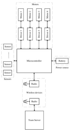
The architecture of a RoboCup small size league system consists of four main components: a single common vision system, a team server for each team, a single referee box and a number of remotely-controlled robots for each team [29]. The vision system consists of overhead cameras connected to a vision processing application that analyzes the captured images to extract location coordinates of the ball and all the robots in the field. The team server runs artificial intelli-gence software that controls the robots over wireless links. The robot includes mechanical parts and electronic circuits controlled by an embedded system. The embedded system works as a mediator between the robot electronics and the team server. It receives and interprets commands sent by the server and drives the robot accordingly. Devices controlled by the embedded system include motors, sensors, and wireless modules. A brief overview of the RoboCup-SSL system is illustrated in Figure1.
A. HARDWARE ARCHITECTURE
A typical RoboCup-SSL robot is made of hardware such as a microprocessor, a radio device, sensors, motors, wheels and gears, battery, a dribbler and a kicker. The dribbler is a special motorized mechanical device that maintains ball possession and release, whereas the kicker is used to kick the ball. As our main target of this study is to implement an embedded system for accurate motion control of omnidirectional mobile robot, the dribbler and kicker devices are not discussed in this research. A gyroscope and an accelerometer are used to measure the instant robot velocity as a feedback source for motion control whereas the infrared sensors are used for ball detection and obstacle avoidance. The radio devices are used
FIGURE 1. System overview of RoboCup-SSL.
FIGURE 2. Hardware architecture.
for wireless communications. For each robot, the essential mechanical parts are the four omni-wheels with gears, and four brush-less DC motors. The hardware architecture of the embedded system is shown in Figure 2. ZigBee wireless modules can be used as radio devices where the ZigBee PRO 2007 protocol is used between multiple ZigBee mod-ules. The sensors can be connected with the microcontroller using SPI, I2C, or UART communication hardware inter-faces. The motors can be driven through motor drivers using
PWM or analog signals generated by the miocrocontroller. An appropriate battery is required as a power source for the devices.
FIGURE 3. Software architecture.
B. SOFTWARE ARCHITECTURE
The software architecture of the embedded system is shown in Figure 3. This system architecture assumes no FPGA. Some software components are implemented FPGA by other teams, e.g. motor control. The firmware consists of motor, sensor, wireless and battery control modules, all of which are executed on the microcontroller which is written in a system programming language such asC. A brief description of the software modules are given below.
• Central Control: The main() function is in the central control unit. The main function calls the required func-tions from related libraries and passes the parameters to accomplish a defined task.
• Sensor Control: There is a sensor library to process the
sensor data. The sensors are connected using any of the hardware connection interfaces to the microcontroller. Similarly, the main controller program communicates with sensor library using some user defined function.
• Wireless Control: A wireless control library acts as a driver for the wireless devices to the microcontrollers. The radio devices can be connected to the microcon-troller using various hardware interfaces like UART, I2C or SPI. The main role of the wireless library is to communicate, control the data flow, and manage buffers.
• Battery Control: A battery or series of batteries are used
as a power source. The main role of the battery module is to supply power at a constant rate and protect the main electric circuit board from over current.
• Motor Control: The most important part of the firmware
is the motor control module. After receiving the com-mands form a wireless link, it decomposes the speed for each wheel. This module calculates a range of floating point parameters (from 0 to 255) of required PWM or analog signal. The microcontroller generates the required voltage to drive the motors with a targeted speed. Also, this module implements a PI or an LQR controller as the low-level motor controller where it gets the feedback from motor encoders or sensors.
C. OPERATION
When the team server decides to move a robot to a target location, it sends a message containing vector data (e.g. target location, speed, and direction) to the radio device through a high-level communication protocol such as ZigBee PRO. Then, a radio device (e.g. ZigBee) forwards this message to the microcontroller for calculating speed, direction and angular velocity of each wheel. The microcontroller sends the required signals to the motor drivers that produce the required analog signals according to the target velocity of the robot to rotate the motors. A feedback signal generated by a motor encoder or sensors is used to monitor the speed accuracy.
IV. OMNIDIRECTIONAL MOTION CONTROL
Motion control of an omnidirectional mobile robot is a chal-lenging task because its kinematics and dynamics are more complex compared to a traditional two wheeled mobile robot. The omnidirectional robot can move in any direction without rotating its body. Considering this, we developed kinemat-ics and dynamkinemat-ics models. Two commonly used controllers for controlling the wheel’s angular velocity are Proportional Differential (PD) and Proportional Integral (PI) controllers. PI controllers are much easier to build, but they do not ensure the reliability if the field friction has varieties [30]. There-fore, we propose using a more advanced controller, namely alinear quadratic regulator(LQR) controller, to control the wheel’s speed as a low-level controller that runs locally on the robot. Also, a fuzzy tuned PI controller is used as a high-level controller to control the position of the mobile robot. The high-level controller determines the robot’s veloc-ity and acceleration. The LQR -low-level controller- reads actual motor speed using motor encoders and uses them as a feedback source. On the other hand, the vision system is used as a feedback source to the high-level fuzzy tuned PI controller. The objective of these controllers is to minimize robot position error. The position error is the distance between the target point and the actual point.
A. ROBOT MODELS
The robot is driven by four motors, and has a cylindrical shape. In the robot models, two different frames are used: the robot body, denoted byb, and the global frame, denoted by g. The frame is a location coordinate vector in a x-y plane. When the robot starts moving, the body frame never changes with respect to its center. Similarly, the global frame is also fixed on the playing field.
1) ROBOT KINEMATICS
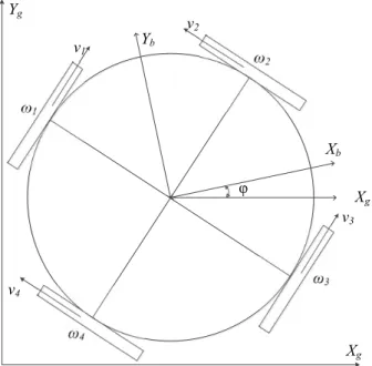
An accurate kinematic model is a prerequisite for performing an accurate trajectory following task using an active motion controller. The following sections discuss the relationship between different geometrical specifications and robot speed with basic kinematic formulas. The position and orienta-tion of the model robot in body and global coordinates are
FIGURE 4. Local and global coordinates.
illustrated in Figure4.
Xb=xb yb φT Xg=xg yg φT (1) The rotation matrixgbR, which is used to change the coordi-nates from the body frame to the global frame, is articulated as g bR= cosφ −sinφ 0 sinφ −cosφ 0 0 −0 1 (2)
The angular velocity and wheel geometry in the global coor-dinates (which is closely associated to the velocity vector) is expressed as
˙
Xg= gbRX˙b= bgR(GT)−1rωL (3) Here, the geometrical matrixGis
G=
−sinθ1 −sinθ2 −sinθ3 −sinθ4
cosθ1 cosθ2 cosθ3 cosθ4
l l l l
(4)
Where,Gwill have fixed values based on the robot geometry and the wheel’s anglesθ1 toθ4. It is used for transforming
the velocity command from the robot’s speed to the rotational speed of the wheel. The mathematical description of the the robot’s acceleration vector is given in Eq. (5), taking the time derivative of Eq. (3) ¨ Xg= gbR˙(G T)−1rω L+ gbR(G T)−1rω˙ L (5)
Gear ratio, robot geometry, and matrix elements are used to estimate the robot’s angular velocity.
2) ROBOT DYNAMICS
In this section, robot dynamics - the relationship among the motor driver’s torque, actuating voltage, angular velocity, and angular acceleration - is described. Moreover, the required dynamic equations of the four-wheeled omnidirectional robot are given. Nonlinearities like motor dynamic constraints may seriously disturb the robot’s performance particularly during accelerating and deceleration [31]. To solve this problem, a model is proposed that considers the nonlinear parameters that are important in controller designing. The relationship matrix between traction force and applied force is as follows
Fb=GFt (6)
The traction force matrix of an experimental robot is Ft =
f1 f2 f3 f4T (7)
Here, fi is the wheel’s traction force values. The moment matrix and the functional forces can be inscribed as
Fb=Fbx Fby TzT (8) The dynamic equation of the traction force of the robot is estimated from Eq. (9):
Ft =G−1gbR Tmhg bR˙(G T)−1rω L+gbR(G T)−1rω˙ L i T (9) Considering entire load and the rotational inertia of the motor, the required torque of the driver is
τm = (Jm+ JL n2)I4×4+ r2 n2G −1g bR Tmg bR(G T)−1 ˙ ωm + (cm+ cL n2)I4×4+ r2 n2G −1g bR Tmg bR˙(G T)−1 ωm (10) Eq. (11) can be simplified as follows; the matrix elements of Z and V are listed in Appendix.
τm=Zω˙m+Vωm (11)
Matrices Z and V are given in Eqs. (12) and (13)
Z = k1 k2 k3 k4 k2 k1 k4 k3 k3 k4 k5 k6 k4 k3 k6 k5 (12) V = k7 −k8φ˙ k9φ˙ k10φ˙ k8φ˙ k7 −k10φ˙ −k9φ˙ −k9φ˙ k10φ˙ k7 −k11φ˙ −k10φ˙ k9φ˙ k11φ˙ k7 (13)
Developing an overall visualization of the torque control method requires drivers dynamic behavior, actuating voltage, back EMF, terminal resistance, and the torque constant. The relationship between them can be written as
τm=(E−EM·ωm)
km
Rt
(14)
Combining Eq. (11) with (14) results in a coupled nonlinear motion equation as follows:
E=(Rt km
Z)ω˙m+(Rt km
V +EM·I4×4)ωm (15) Eq. (15) illustrates the relationship of dynamic behavior and driver that plays a crucial role in modeling.
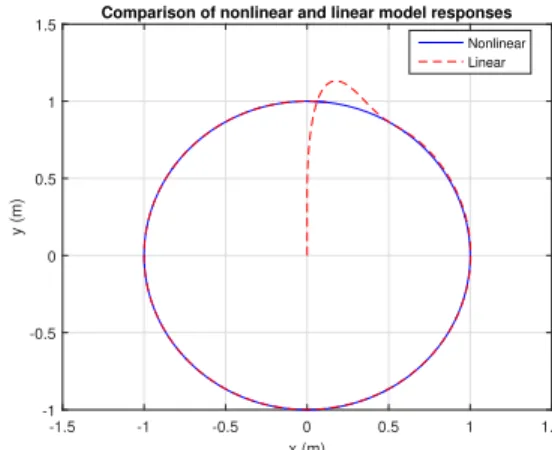
FIGURE 5. Comparison of linear and nonlinear model responses: Circular trajectory.
FIGURE 6. Comparison of linear and nonlinear model responses: Rectangular trajectory.
B. ROBOT MODEL LINEARIZATION
The previous sections discussed that the omnidirectional mobile robot is a nonlinear system where robot nonlinearity comes from the friction and the motor voltage limits [31]. These nonlinearities are visible during concurrent linear and rotational path. Therefore, it is practical to estimate a linear model that establishes the system motion equations. For a controllable nonlinear system, a linear controller, especially when augmented with integral controller, is always powerful in stabilizing a nonlinear system especially with suitable selection of the parameters. We have linearized our nonlinear system and then tune the desired fuzzy-PI controller since it helps to decrease and minimize deviations from nonlin-earity. As a result, Figure5 and Figure 6 present compar-ison between the linear and nonlinear performance in two
FIGURE 7. Configuration of fuzzy adaptive PI.
FIGURE 8. Membership function plotting of of E, EC.
trajectory following tasks: one circular and one rectangular path with time variation. The linearized model offers more satisfactory outcome with a maximum deviation of 6.7% in ensuring the correct track than the nonlinear method. This result has a minor effect on robots current positioning in the field with approximately 1.5% error.
C. CONTROLLER DESIGN
To achieve an accurate and efficient drive, two closed loop controllers are employed in the proposed motion control approach. The LQR that estimates the optimal input for the motor drivers is executed on the robot main board, whereas the fuzzy adaptive PI controller to calculate the right pathway runs on the team server.
1) LOW-LEVEL CONTROLLER
Optimal performance with low-energy is a popular topic for mobile robots [32]. An optimal control system is generally defined as a system which delivers maximum return for a minimum cost [33]. Presently, there are two leading methods for implementing optimal controllers: tracking control and regulator control [34]. Tracking control focuses on a defined state-time history in a way so as to optimize a specified
FIGURE 9. Membership function plotting of1KPand1KI.
TABLE 1.Fuzzy rules forKP.
TABLE 2.Fuzzy rules forKI.
performance index whereas regulator control returns the system to the equilibrium state [35]. The regulator control approach delivers an ideal solution to minimize the distance between the targeted path and the actual trajectory [36]. The following paragraph explains the characteristics of a discrete time linear quadratic regulator controller that will be applied in this study to follow the reference path for the omnidirec-tional mobile robot [37].
FIGURE 10. Fuzzy-PI path planner and LQR controller schematic.
FIGURE 11. Optimal voltage for motors on the rectangular trajectory for PI and LQR controllers. The state equation is used to describe the time-invariant
and linear system
x(k+1)=Ax(k)+Bu(k) (16) with the output
y(k)=Cx(k) (17) Eq. (18) presents the relationship among the control variables and parameters [38]. It indicates that the performance index must be minimized. J = 1 2 Cx(kf)−z(kf) T FCx(kf)−z(kf) +1 2 kf−1 X k=k0 {[Cx(k)−z(k)]TQ[Cx(k)−z(k)] +uT(k)Ru(k)} (18)
where ann-order and anr-order state, a control, and an output vectors are denoted asx(k),u(k) andy(k) respectively. The positive semi-definite symmetric matricesF andQof size n×n, and the positive definite symmetric matrixR of size r×r, are defined. The conditionx(kf) is free with fixedkf. The initial condition x(k0) is given to minimize the error
e(k)=y(k)z(k), wherez(k) is ann-dimensional target matrix. The formulation of Hamiltonian is
H(x(k),u(k), λ(k+1)) = 1 2 kf−1 X k=k0 {[Cx(k)−z(k)]TQ[Cx(k)−z(k)] +uT(k)Ru(k)}λT(k+1)[Ax(k)+Bu(k)] (19) where, x? and λ? are used in state and costate equations. All related calculations come from Hamiltonian equations,
as expressed in Eqs. (20)-(23), where the star indicates the optimized parameter.
δH
δλ ?(k+1) =x?(k+1) (20)
x?(k+1)=Ax?(k)+Bu?(k) (21) The costate equations from Hamiltonian are stated as
δH
δx?(k) =λ ?(k) (22)
λ ?(k)=ATλ ?(k+1)+Vx?(k)−Wz(k) (23) The final condition is
λ(kf)=CTFCx(kf)−CTFz(kf) (24) Thus, we can get the optimal voltage for four motor drivers by minimizing the Hamiltonian considering the control input in open loop.
δH
δu?(k) =0 (25)
u?(k)= −R−1BTλ ?(k+1) (26) By implementing Eqs. (25) and (26) in the state, a canonical system is derived from costate systems as
x?(k+1) λ ?(k) = A−E VAT x?(k) λ ?(k+1) + 0 −W z(k) (27) Here,E =BR−1BT,V =CTQC andW =CTQ. By elimi-nating the costate variable:
λ ?(k)=P(k)x?(k)−g(k) (28) deducing the costateλ ?(k) yieldsP(k) andg(k) stated as
P(k)=ATP(k+1)[I+EP(k+1)]−1A+V (29) g(k)=nAT −ATP(k+1) [I+EP(k+1)]−1Eo
g(k+1)+Wz(k) (30) Terminator constraints are also given in Eqs. (31) and (32).
P(kf)=CTFC (31)
g(kf)=CTFz(kf) (32) The nonlinear Difference Riccati Equation (DRE) in Eq. (29) to get an acceptable solution of backwards consid-ering the target constraint (31). Also, the linear vector differ-ence in Eq. (30) solves backwards using the final condition (32). These outcomes are achieved offline to be implemented in closed loop control method, expressed as:
u?(k)= −L(k)x?(k)+Lg(k)g(k+1) (33) The gains Lg(k)-forward and L(k)-back, are stated in Eqs. (34) and (35). L(k)=hR+BTP(k+1)B i−1 BTP(k+1)A (34) L(g)=hR+BTP(k+1)Bi −1 BT (35)
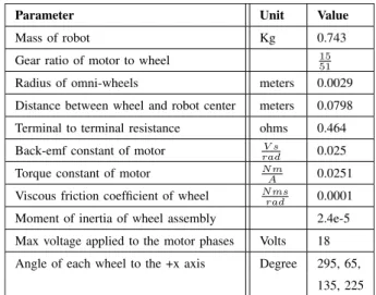
TABLE 3.Robot model parameters and values.
As a result, the optimized path is stated in Eq. (36)
x?(k+1)=[A−BL(k)]x(k)+BLg(k)g(k+1) (36) The earlier closed-loop controller can follow the target path accurately, but in the existence of disturbance, there is a deviation between the desired and actual path. To tune the PI that can quickly stabilize the erratic system with a constant disturbance, a fuzzy control logic is used.
2) HIGH-LEVEL CONTROLLER
The preceding section discuss linearization and a consistent routine for velocity profile determination. The LQR approach is used without a high-level controller such as a fuzzy logic controller (FLC). However, this section discusses how the fuzzy path planner and controller schemes are implemented as a high-level position controller.
If the current position of the robot is not the target position, the distance function calculates the gap between the target and actual position. In this study, a PI controller is used to control the position of the omnidirectional mobile robot which is tuned by a Fuzzy Logic Controller (FLC) [39]. As a result of applying linearized PI with FLC, the position errors of a tracked path are significantly reduced, which is described arithmetically in sectionV. There are two major enhance-ments being realized in fuzzy adaptive PI path planner engag-ing the LQR. First, employengag-ing the FLC to optimize the PI parameters improves the trajectory following performance of omnidirectional mobile robots, and other enhancement miti-gates the location and travel time error pointedly. To achieve a specified performance using PI controller, selecting a suitable value for thePandI coefficients of the PI controller is an important task, which can be done automatically by using an FLC. However, FLC can be adjusted by either regulating the input-output gains of the control system or changing the position of linked membership functions alike [40], [41]. 3) PI CONTROLLER
In this study, we consider only PI controller. PI controller is a wildly used control system in many complex systems because
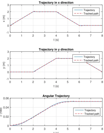
FIGURE 12. The difference between tracked path and trajectory on a circular pathway by the LQR controller with robot velocityVrobot=1m/s φ=0.05rad/s.
it is easy to implement. The stable time can be minimized by tuning the values of thePandI coefficients denoted by KP and KI. The mathematical linear relationship between the output, u(t) and the error e(t) can be expressed by the following equation:
u(t)=Kpe(t)+KI Z
e(t)dt (37) where the proportional and integral gains are denoted by KP and KI. One of the common approaches to tune the values of PI controllers is the Ziegler-Nichols method [42]. In this research, the constraints of the PI controller are set toKP=10,KI =0.5.
4) FUZZY ADAPTIVE PI CONTROLLER
The fuzzy logic unit consists of two inputs: the erroreand the change in the errorec. The outputs1KP and1KI are denoted as the changes of the proportional gainKPand the integral gainKI. The three key elements of the fuzzy adaptive PI are fuzzification, fuzzy inference and defuzzification, all of which are illustrated in the schematic diagram in Figure7. First, to convert the input and output values to semantic variables, a fuzzification of the input and the output variables is employed where the fuzzy range of the variables is e [−1,10],ec[−1,10],1KP[1,1.5], andKI[0,1.5]. More specifically, the fuzzy variety is segmented into seven seman-tic variables, and the equivalent fuzzy subsets aree,ec, 1KP,
FIGURE 13. Robot position and orientation variation in rectangular trajectory.
FIGURE 14. Surface area curve of fuzzy controller for input signals.
1KI = [NB,NM,NS,ZO,PS,PM,PB] where NB: Neg. Big, NM: Neg. Middle, NS: Neg. Small, ZO: Zero, PS: Pos. Small, PM: Pos. Middle, and PB: Pos. Big.
Every membership functions are set to the Gaussian curve. Figure8 and Figure9present the fuzzy membership func-tions. A key step in designing a fuzzy control logic is the formation of a fuzzy inference rule among the input variables e,ec and the output variables1KP and1KI based on the information and skill of input-output data. In this research, the rules of PI parameters are applied in team server and, through simulation and experiment the value for P and I are extracted. The fuzzy laws are concise in Table1 and2. According to Table 1, total forty-nine laws can be formu-lated as follows: If e is Ai and ec is Bj, then 1KP/1KI
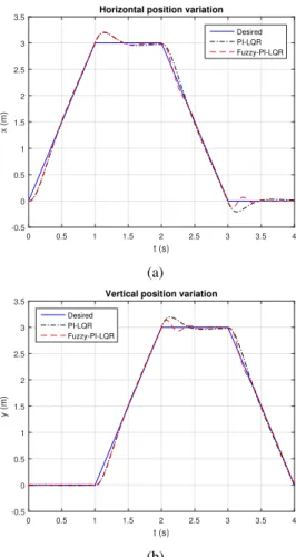
FIGURE 15. The accuracy of rectangular path following for robots transitional speed (a) 3 m/s; (b) 4 m/s.
is Cij/Dij whereAi,Bj,Cij,Dij are equivalent to the fuzzy subsets of e,ec, 1KP, 1KI. To achieve the fuzzy interfer-ence, the Mamdanis Min-Max is employed. For example, the degree of membership of the fuzzy subsets Cij for the parameter1KPcan be obtained as follows:
uc(1KP)= ∨7i,j=1
[ui(e)∧uj(ec)]∧ucij(1KP) (38) Where ux is the degree of membership. Defuzzification is the procedure of converting fuzzy inputs to crisp data. To get the crisp values, the center of gravity approach is applied. The coefficient1KP(1KIis similar) might estimate as follows.
1KP(e,ec)= P7 k=11KPuc(1Kp) P7 k=1uc(1Kp) (39) After defuzzification, the parametersKP,KI can be derived:
KP =KP0+1KP (40)
KI =KI0+1KI (41) WhereKP0,KI0are the actual coefficient ofPandI.
V. SIMULATION RESULTS
Matlab simulink 2015 software simulates the four-wheeled omnidirectional mobile robots using FLC tuned PI and
FIGURE 16. The horizontal and vertical deviations as the output of both PI-LQR and fuzzy-PI-LQR controller for the speed of 3 m/s.
LQR controllers. A brief schematic diagram of the FLC tuned PI controller with the trajectory planner, and the LQR controller are shown in Figure10. A circular or rectangu-lar trajectory is defined in the path planner that generates the target positions continuously. The velocity filter checks the transitional and rotational velocity/acceleration limit to avoid damage. The fuzzy adaptive PI controller estimates an accurate target position based on the robot’s current posi-tion, therefore, minimizing the position error. Then inverse kinematics derive the robot body velocity from the global velocity. The output of LQR controller is an optimal set of input voltage for the motors based on model specification such as robot mass, motor inertia, etc. According to the robot dynamics, the robot starts moving to reach the desired point. Feedback from two sources is used in this simulation. First, current velocity of the robot is fed into LQR to calculate the new velocity vector. Second, position feedback is used in FLC to make an accurate path planning. Finally, the FLC generates a set of optimal voltages for PI controller depending on the value of tracking erroreand change in errorec.
The initial parameters of the robot model are listed in Table3. The parameters are used to configure the LQR con-troller. The primary concern of employment of LQR was to make the model linearized. An integrator is used on the error
FIGURE 17. The comparison of robot orientation error in both cases with the velocity (a) 3 m/s; (b) 4 m/s.
FIGURE 18. The positional error analysis for both PI-LQR and fuzzy-PI-LQR controller on a circular trajectory for robot velocity V=4m/s.
matrix in the low-level controller. This approach is energy efficient because it estimates the optimal voltage for each motor driver to drive with minimum tracking error. Figure11
illustrates the desired voltage and controllers output for a particular rectangular trajectory. Figure12and Figure13give an impression of path planning consequences for rectangular and circular trajectory as two different pathways where the
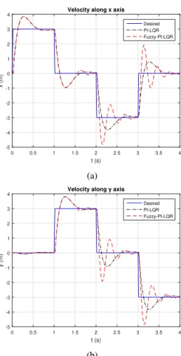
FIGURE 19. The velocity norm in both horizontal and vertical in 3 m/s. robots translational and rotational speed are same (1 m/s and 0.05 rad/s). The preliminary simulation results ensure that the robot can follow the desired path with a slight deviation.
The robot’s global position on the playground and the wheels’ angular speed are estimated according to kinematics equations. In contrast, quick fluctuations in the path-following led to added slip of wheels, as is noticeable in Figure13 which displays the relationship between the geometric coordinate of a pathway and the robot’s position. The results are 1.1% mean position and 3.2% orientation deviation. Furthermore, it is clearly observed that the error is decreases along the straight pathways that validate proper PI value selection of high-level position controller. The fuzzy controller behavior surface that presents the correlation between the input parameters (E,EC), and corresponding output results asKp andKI value are graphically depicted in Figure 14. The path-following characteristics of experi-mental model with PI-LQR and fuzzy-PI-LQR schemes is presented in Figure15. The detected undulations in the speed curves at the corners are ascribed to adjusting the robot in given trajectories with encounter path’s geometrical require-ments and robot dynamics.
Figure15shows that the max. deviation along y-axis and x-axis are 9.0% and 3.4% respectively for the PI-LQR approach with velocity of 3 m/s, and can be augmented to
TABLE 4. Comparison of velocity norm with existing literature for the two path planners.
FIGURE 20. The deviation from targeted trajectory in presence of randomly distributed disturbance on rectangular trajectory for the transitional speed of (a) V = 2 m/s; (b) V=4 m/s.
10.6% and 6.7% if the velocity is 4 m/s. The existence of the Fuzzy logic controller on the maneuver planner diminishes the deviations to 6.6% and 1.2% for the velocity of 3 m/s trajectory and 8.7%, 0.9% for above the acceptable velocity. A performance comparison between this study and existing research for the same controllers is given in Table5. There is a satisfactory steadiness between the targeted path and the
TABLE 5.Error comparison with existing literature.
fuzzy-PI-LQR controller’s outcome at slower speeds such as 3 m/s, but deviation will be increased if speed is high, i.e., 4 m/s. It is observed from Figure15that the established fuzzy-PI-LQR controller offers a further accurate perfor-mance compared to the PI-LQR approach for permissible high slip-free speed. The outcomes of vertical and horizontal travels without noise are drawn in Figure 16. The tracked maneuver depicts the performance along the x-axis where it ends up with an error of up to 9.7% and 11.9% at a initial high-pitched edge, which indicates benefits of FLC at any speed. The gap between targeted path and tracked path for velocity 3 m/s may be clarified by the proximity and the highest acceptable speed. However, inconsistencies are enlarged at high velocities, as illustrated in Figure 15b. The presented LQR method as low-level control system has monitored the robot’s orientation that led to a tolerable error in contrast to the robot’s nonlinear model. The relationship between geometrical track and robot orientation in the case of the rectangular path for both 3 m/s and 4 m/s are illustrated in Figure 17. It is clear that a sharp direction change is observed in robot alignment variation in a rectangular maneu-ver. These vicissitudes led the robot to slip slightly, partic-ularly for velocity above the max. estimated in SectionIV, as depicted in Figure 17b. These vacillation amplitudes are nearly 50% of those seen without the FLC.
For the sake of analyzing the deviation, a circular maneuver is created using two existing trajectory planners, and the outcomes are depicted in Figure18, where the error varia-tions of both approaches are illustrated. The slight fluctuation
FIGURE 21. Error analysis on the rectangular maneuver with external load with the velocity of (a) 3 m/s; (b) 4 m/s.
detected on the proposed method caused input and output rule segmentations. In Figure 19, there is an inclination of velocity increase and decrease respectively near the angular points that appears rational based on the stated pathway. In Figure 20, the expected outcomes for the FLC trajectory planner are illustrated in the presence of randomly distributed disturbance applied for both trajectory planners with fre-quency and amplitude of 1 rad/s and 0.01m respectively. The difference between orientation and position error with external loads for the traditional trajectory-following task is demonstrated in Figure21. The experimental measurement
FIGURE 22. Circular Trajectory with s=4 m/s.
FIGURE 23. DNA shape trajectory with s=2 m/s.
is studied with a marginal slip-free velocity of 4 m/s. Robot position, orientation and motion smoothness of target and tracked path following with the external noise are depicted in Figure21. Finally, the deviation between targeted path and tracked path of a hard and smooth trajectories is shown in following graphs. A circular trajectory following outcome is shown in Figure22. Two asymmetric trajectories, specifically DNA (Deoxyribonucleic Acid) and flower shaped trajecto-ries, with the velocity of 2 m/s are depicted in the Figure23
and Figure 24 respectively. Initially, PI-LQR and fuzzy-PI LQR perform similarly, but the stable time of fuzzy adap-tive PI-LQR is much less than the PI-LQR. The standard deviations of the desired velocity norm(σVnd), the velocity norm error(σeVn), and the maximum error of the velocity norm(eVnmax) are given in Table4 for three different robot speed conditions. The lower standard deviation observed for the fuzzy-PI-LQR approach for all three maneuvers, espe-cially with the presence of noise, rationalizes employing this method which leads to lower fluctuations of desired velocity norms.
VI. EXPERIMENTAL RESULTS
A four-wheeled omnidirectional RoboCup-SSL robot is made to do the experiment with the proposed control system.
FIGURE 24. Flower shape trajectory with s=2 m/s.
FIGURE 25. Mechanical drawing of the robot.
An experimental execution of the embedded system for con-trolling the motion is described in this section.
A. ROBOT ASSEMBLY
Two XBee modules (router AT and coordinator AT) with baud rate 9600 were used for wireless communication. Four motor drivers were used with a maximum rotational speed of 625rpm. There is an inner closed loop to control the angular velocity of the wheels using PI controller based on the motor encoder feedback. Moreover, an HD web-cam was used for vision feedback for position tracking. The robot pro-totype was made of high-quality plastic to minimize weight. To avoid short circuit problems among the electrical compo-nents and decrease losses, every part was hardened anodized. The diameter, height and weight of the robot were 178mm, 138mm and 0.75kg respectively. The mechanical design of the robot is shown in Figure25. Each wheel of the robot was driven by a BLDC motor. The motor power was transmitted via two gears with a ratio of 51:15. The wheel diameter, roller
FIGURE 26. Omnidirectional robot.
FIGURE 27. Omnidiretional robot with color code.
diameter, load capacity, and net weight are 58mm, 13mm, 3kg, and 60g respectively. A brush-less DC motor with a maximum speed of 10000rpm was used to rotate the wheel. Also, it had a hall sensor used to get the rotation feedback of an internal close loop. To establish a reliable wireless communication between the robot and the team server, a low power 2.4GHz XBee s2c ZigBee module was connected to the team server and another one on each main board, which is operated in ZigBee PRO 2007 protocol. It had 16 channels and is capable of 128-bit encryption. There was a bidirec-tional communication existing to receive velocity commands from the team server and to send the feedback. An illustration of the model robot is shown in the Figure26.
B. EXPERIMENTAL SETUP
The complete procedure of the experimental test bed is described in this section. Before starting the experiment, it was necessary to check the pin configuration and fix the message format. Four motor drivers and one XBee were
TABLE 6. Error comparison.
connected to the main microcontroller Arduino Due board. The most important pin of every driver module is 26(speed) which is connected to the PWM pins(2-5) of Arduino. The direction pin(23) of the driver required digital binary high or low signal, so it was connected to the digital pin(34-37). The enable(22) pin also needed a digital sig-nal. Thus, it was connected to the pins(22-25). To set the motor speed range, the digital input pins N1(20) and N2(21) were connected to pins(40-49). Finally, the ready pin is an output digital signal from the driver which is connected to pins(28-31). The motors, and radio devices had been initial-ized at the beginning of the firmware. Then, a test packet was sent and received between the robot and team server to con-firm the wireless communication. There were several tasks that had to be accomplished concurrently such as reading commands, running the motor and sending feedback. To do the multitasking, we used multi-thread. Although Arduino does not support ‘‘REAL’’ parallel tasks (aka Threads), we can make use of the library (ivanseidel) to schedule tasks with fixed (or variable) time between runs [43]. Once the motor is ready, the controller sent PWM signal to each motor sequentially based on the target velocity of the robot. An internal close loop adjusted the motor speed using PI controller. Also, the monitornpin in the motor driver helped to know the motor’s current speed. A recent velocity feedback was received from the motor encoder to feed into low-level velocity controller for calculating the targeted PWM signal for each motor.
FIGURE 28. Circular trajectory with max. allowable speed.
C. RESULTS AND DISCUSSION
The robot’s experimental performance of a circular trajectory following is recorded with a maximum allowable speed and is shown in Figure28. The position and orientation variation
FIGURE 29. Position error comparison.
FIGURE 30. DNA trajectory with max. allowable speed.
FIGURE 31. Position error comparison.
of this trajectory are illustrated in Figure29. The maximum deviation along the x-axis and y-axis are 4.99% and 16.01% respectively and is listed in Table 6. Similarly, a critical asymmetric maneuver is created for measuring the position and orientation errors between targeted path and actual path which is illustrated in Figure30. Also, the position errors of this trajectory is presented in the Figure31. The maximum deviation along y-axis and x-axis movement are 9.60% and 17.96% respectively for the Fuzzy-PI approach with velocity
of 1 m/s that is augmented to 5.17% and 19.66% for a pathway with the maximum allowable velocity in Figure 31. The existence of the FLC on the maneuver planner diminishes this deviations.
VII. CONCLUSION
In this research, a simple and easy-to-use embedded system is developed for controlling the motion of four wheeled omni-directional mobile robots using two closed loop structure control systems that can successfully read commands from the team server and execute received commands to drive the robot accurately and efficiently in an x-y plane. The outer loop controller, a fuzzy adaptive PI, calculates the accurate target position and minimizes tracking errors using vision feedback. Concurrently, an inner loop controller, a discrete time linear quadratic regulator is employed on the robot to obtain the optimal input for the motor drivers to help the robot to run with an exact wheel speed in an energy efficient way. An essential contribution illustrated in this research is an improved performance in the combination of fuzzy tuned PI with LQR controller over classic PI controller. Furthermore, a conducted simulation and experiment with and without external load yield an optimal outcome that ensured the pro-posed claim.
APPENDIX A NOMENCLATURE
E Voltage matrix [E1 E2 E3 E4]t
EM Back EMF
Ft Traction force matrix [f1 f2 f3 f4]
Fb Force and moment on the robot in the moving frame [FbxFbyTz]
Fg Force and moment on the robot in global coordinates [FxFyTz]
G Geometrical matrix Jl Wheel’s inertia
Jm Driver’s rotor inertia
J Robot’s inertia
Rt Driver’s terminal resistance phase to phase g
bR Rotation matrix
Tz Applied moment on the robot about vertical axis
Xm Local position matrix, [xmymφ]T
Xg Global position matrix, [xgygφ]T
˙
Xg,X˙b,V Global and local velocity
¨
Xg,X¨b,a Global and local acceleration
km Driver’s torque constant
cm Coefficient of damping of the driver
cL Coefficient of damping of the wheel
l Wheel base m Robot’s mass n Gear ratio r Wheel radius
θ Angle of wheels with respect to local coordinates
τm Drivers torque matrix, [τm1τm2τm3τm4]T
˙
φ Angular velocity of the robot
ωm Angular velocity matrix of the drivers
˙
ωm Angular acceleration matrix of the drivers
ωL Angular velocity matrix of the wheels
˙
ωL Angular acceleration matrix of the wheels APPENDIX B k1 =Jm+ JL n2 + r2 n2(0.3m+11.80J) k2 = r2 n2(0.03m+11.8J) k3 = r2 n2(−0.25m+9.1J) k4 = r2 n2(−0.06m+9.1J) k5 =Jm+ JL n2 + r2 n2(0.23m+7J) k6 = r2 n2(0.7m+7J) k7 =cm+ cL n2; k8=0.3 r2 n2m; k9=0.02 r2 n2m; k10 =0.26 r2 n2m; k11=0.24 r2 n2m ACKNOWLEDGMENT
The authors would like to thank the Department of Computer Engineering, KFUPM for arranging necessary equipment and lab facilities for this experiment. Also, authors want to thanks to the team members of KFUPM RoboCup-SSL for benevo-lently providing the experimental support from their area of expertise.
REFERENCES
[1] L. Iocchi, H. Matsubara, A. Weitzenfeld, and C. Zhou, Eds.,RoboCup 2008: Robot Soccer World Cup XII, vol. 5399. Berlin, Germany: Springer-Verlag, 2009.
[2] U. Visser, F. Ribeiro, T. Ohashi, and F. Dellaert, Eds.,RoboCup 2007: Robot Soccer World Cup XI, vol. 5001. Berlin, Germany: Springer-Verlag, 2008.
[3] (2017).Small Size League. [Online]. Available: http://wiki.robocup.org/ Small_Size_League
[4] S. Zickler, J. Biswas, K. Luo, and M. Veloso, ‘‘CMDragons 2010 team description,’’ Carnegie Mellon Univ., Pittsburgh, PA, USA, Tech. Rep., 2010.
[5] D. Hanselman,Brushless Motors: Magnetic Design, Performance and Control. Orono, MN, USA: E-Man Press LLC, 2012.
[6] B. Perunet al., ‘‘Tigers Mannheim’s Team description for RoboCup 2011,’’ Duale Hochschule Baden-Württemberg Mannheim, Mannheim, Germany, Tech. Rep., 2011.
[7] (2017).FreeRTOS. [Online]. Available: www.freertos.org
[8] K. Sukvichai, T. Ariyachartphadungkit, and K. Chaiso, ‘‘Robot hardware, software, and technologies behind the skuba robot team,’’ inRoboCup: Robot Soccer World Cup XV. Berlin, Germany: Springer-Verlag, 2012, pp. 13–24.
[9] C. Röhrig, D. Heß, C. Kirsch, and F. Künemund, ‘‘Localization of an omnidirectional transport robot using IEEE 802.15.4a ranging and laser range finder,’’ inProc. IEEE/RSJ Int. Conf. Intell. Robots Syst. (IROS), Oct. 2010, pp. 3798–3803.
[10] X. Li and A. Zell, ‘‘Motion control of an omnidirectional mobile robot,’’ inInformatics in Control, Automation and Robotics. Berlin, Germany: Springer-Verlag, 2009, pp. 181–193.
[11] R. Rojas, ‘‘Omnidirectional control,’’ Freie Univ. Berlin, Berlin, Germany, Tech. Rep., 2005.
[12] J. Buchanan, S. Csukas, L. Langstaff, R. Strat, and R. Woodworth, ‘‘Robo-Jackets 2014 team description paper,’’ Georgia Inst. Technol., Atlanta, GA USA, Tech. Rep., 2014.
[13] K. Sukvichai, P. Wasuntapichaikul, and Y. Tipsuwan, ‘‘Implementation of torque controller for brushless motors on the omni-directional wheeled mobile robot,’’ inProc. ITC-CSCC, 2010, pp. 19–22.
[14] K. Sukvichai and P. Wechsuwanmanee, ‘‘Development of the modified kinematics for a wheeled mobile robot,’’ inProc. ITC-CSCC, 2010, pp. 88–90.
[15] Z. Chen and S. T. Birchfield, ‘‘Qualitative vision-based path following,’’ IEEE Trans. Robot., vol. 25, no. 3, pp. 749–754, Jun. 2009.
[16] T. Kalmár-Nagy, R. D’Andrea, and P. Ganguly, ‘‘Near-optimal dynamic trajectory generation and control of an omnidirectional vehicle,’’Robot. Auto. Syst., vol. 46, no. 1, pp. 47–64, 2004.
[17] O. Purwin and R. D’Andrea, ‘‘Trajectory generation and control for four wheeled omnidirectional vehicles,’’Robot. Auto. Syst., vol. 54, no. 1, pp. 13–22, 2006.
[18] Y. Liu, J. J. Zhu, R. L. Williams, and J. Wu, ‘‘Omni-directional mobile robot controller based on trajectory linearization,’’Robot. Auto. Syst., vol. 56, no. 5, pp. 461–479, 2008.
[19] E. Hashemi, M. G. Jadidi, and O. B. Babarsad, ‘‘Trajectory planning optimization with dynamic modeling of four wheeled omni-directional mobile robots,’’ inProc. IEEE Int. Symp. Comput. Intell. Robot. Autom. (CIRA), Dec. 2009, pp. 272–277.
[20] W. Sun, J. van den Berg, and R. Alterovitz, ‘‘Stochastic extended LQR for optimization-based motion planning under uncertainty,’’IEEE Trans. Autom. Sci. Eng., vol. 13, no. 2, pp. 437–447, Apr. 2016.
[21] S. I. Han and J. M. Lee, ‘‘Balancing and velocity control of a unicycle robot based on the dynamic model,’’IEEE Trans. Ind. Electron., vol. 62, no. 1, pp. 405–413, Jan. 2015.
[22] M. C. Priess, R. Conway, J. Choi, J. M. Popovich, and C. Radcliffe, ‘‘Solutions to the inverse LQR problem with application to biological systems analysis,’’IEEE Trans. Control Syst. Technol., vol. 23, no. 2, pp. 770–777, Mar. 2015.
[23] Z. Kovacic and S. Bogdan,Fuzzy Controller Design: Theory and Applica-tions, vol. 19. Boca Raton, FL, USA: CRC Press, 2005.
[24] I. Iancu, ‘‘A Mamdani type fuzzy logic controller,’’ inFuzzy Logic— Controls, Concepts, Theories and Applications. Rijeka, Croatia: InTech, 2012.
[25] A. Sheikhlar, A. Fakharian, and A. Adhami-Mirhosseini, ‘‘Fuzzy adaptive PI control of omni-directional mobile robot,’’ inProc. 13th Iranian Conf. Fuzzy Syst. (IFSC), 2013, pp. 1–4.
[26] A. G. Ram and S. A. Lincoln, ‘‘A model reference-based fuzzy adaptive PI controller for non-linear level process system,’’Int. J. Res. Rev. Appl. Sci., vol. 4, no. 2, pp. 477–486, 2013.
[27] M. Nie and W. W. Tan, ‘‘Stable adaptive fuzzy PD plus PI controller for nonlinear uncertain systems,’’Fuzzy Sets Syst., vol. 179, no. 1, pp. 1–19, 2011.
[28] F. Abdessemed, K. Benmahammed, and E. Monacelli, ‘‘A fuzzy-based reactive controller for a non-holonomic mobile robot,’’Robot. Auto. Syst., vol. 47, no. 1, pp. 31–46, 2004.
[29] L. A. Martinez-Gomezet al., ‘‘Eagle knights: Small size RoboCup soccer team,’’ inProc. 7th SBAI/II IEEE LARS, São Luís, Brazil, 2005. [30] E. Hashemi, M. G. Jadidi, and N. G. Jadidi, ‘‘Model-based PI–fuzzy
control of four-wheeled omni-directional mobile robots,’’Robot. Auto. Syst., vol. 59, no. 11, pp. 930–942, 2011.
[31] A. S. Conceição, A. P. Moreira, and P. J. Costa, ‘‘Practical approach of modeling and parameters estimation for omnidirectional mobile robots,’’ IEEE/ASME Trans. Mechatronics, vol. 14, no. 3, pp. 377–381, Jun. 2009. [32] D. Meike and L. Ribickis, ‘‘Energy efficient use of robotics in the auto-mobile industry,’’ inProc. 15th Int. Conf. Adv. Robot. (ICAR), 2011, pp. 507–511.
[33] X. Zeng, P. Yi, and Y. Hong, ‘‘Distributed continuous-time algorithm for constrained convex optimizations via nonsmooth analysis approach,’’ IEEE Trans. Autom. Control, vol. 62, no. 10, pp. 5227–5233, Oct. 2017. [34] H.-J. Zhang, J.-W. Gong, Y. Jiang, G.-M. Xiong, and H.-Y. Chen, ‘‘An
iterative linear quadratic regulator based trajectory tracking controller for wheeled mobile robot,’’J. Zhejiang Univ. Sci. C, vol. 13, no. 8, pp. 593–600, 2012.
[35] R.-D. Zhao, Y.-J. Wang, and J.-S. Zhang, ‘‘Maximum power point tracking control of the wind energy generation system with direct-driven per-manent magnet synchronous generators,’’Proc. CSEE, vol. 29, no. 27, pp. 106–111, 2009.
[36] Z. Zhong, R.-J. Wai, Z. Shao, and M. Xu, ‘‘Reachable set estimation and decentralized controller design for large-scale nonlinear systems with time-varying delay and input constraint,’’IEEE Trans. Fuzzy Syst., vol. 25, no. 6, pp. 1629–1643, Dec. 2017.
[37] B. D. O. Anderson and J. B. Moore,Optimal Control: Linear Quadratic Methods. North Chelmsford, MA, USA: Courier Corporation, 2007. [38] D. S. Naidu,Optimal Control Systems. Boca Raton, FL, USA: CRC Press,
2002.
[39] A. Taskin and T. Kumbasar, ‘‘An open source matlab/simulink toolbox for interval type-2 fuzzy logic systems,’’ inProc. IEEE Symp. Ser. Comput. Intell., Dec. 2015, pp. 1561–1568.
[40] K. S. Tang, K. F. Man, G. Chen, and S. Kwong, ‘‘An optimal fuzzy PID controller,’’IEEE Trans. Ind. Electron., vol. 48, no. 4, pp. 757–765, Aug. 2001.
[41] R.-E. Precup and S. Preitl, ‘‘PI-fuzzy controllers for integral plants to ensure robust stability,’’Inf. Sci., vol. 177, no. 20, pp. 4410–4429, 2007. [42] K. J. Åström and B. Wittenmark,Adaptive Control. North Chelmsford,
MA, USA: Courier Corporation, 2013.
[43] Ivanseidel. (2017). GitHub. [Online]. Available: https://github.com/ ivanseidel/arduinothread
MD. ABDULLAH AL MAMUNwas born in 1988. He received the B.S. degree in computer sci-ence & engineering from the Dhaka University of Engineering & Technology, Bangladesh, in 2012, the M.S. degree in computer engineering from the King Fahd University of Petroleum and Min-erals, Saudi Arabia, in 2017. He was a Free-lance Researcher at the Department of Renewable Energy, Research Institute, KUPM, in 2015 and 2016, respectively. He is currently a Graduate Teaching Assistant with Qatar University, Doha, Qatar. His research interests include machine learning, image processing, robot cognitive, and embedded system.
MOHAMMAD TARIQ NASIRreceived the bach-elor’s degree in mechatronics engineering from Jordan University, the master’s degree from the Jordan University of Science and Technology, and the Ph.D. degree from the King Fahd University of Petroleum & Minerals. He is currently an Assis-tant Professor with the Mechanical Department, Applied Science Private University. His research interests lie in the area of robotics, control systems, and automation.
AHMAD KHAYYAT received the B.S. degree (Hons.) from the King Fahd University of Petroleum and Minerals (KFUPM) in 2002, the master’s of science in engineering and Ph.D. degrees from Queens University, Canada, in 2013 and 2007, respectively. He is currently an Assistant Professor with the Computer Engineer-ing Department, KFUPM. He is a member of the IEEE Computer Society.