Importance-Driven Time-Varying Data Visualization

Importance-Driven Time-Varying Data Visualization

Abstract—The ability to identify and present the most essential aspects of time-varying data is critically important in many areas of science and engineering. This paper introduces an importance-driven approach to time-varying volume data visualization for enhancing that ability. By conducting a block-wise analysis of the data in the joint feature-temporal space, we derive an importance curve for each data block based on the formulation of conditional entropy from information theory. Each curve characterizes the local temporal behavior of the respective block, and clustering the importance curves of all the volume blocks effectively classifies the underlying data. Based on different temporal trends exhibited by importance curves and their clustering results, we suggest several interesting and effective visualization techniques to reveal the important aspects of time-varying data.

Index Terms—Time-varying data, conditional entropy, joint feature-temporal space, clustering, highlighting, transfer function.

1 INTRODUCTION

Time-dependent simulations and time-varying data can be found in al-most every major scientific discipline. Time-varying data are dynamic in nature and can be categorized by different temporal behaviors they exhibit. The first category of time-varying data is regular, which usu-ally involves a certain phenomenon that grows, persists, and declines in several (distinct) stages. The rate of change at each stage could vary dramatically in space and time. Many natural phenomena and their simulations, such as the earthquake, fall into this category. The second category of time-varying data is periodic. For this type of data with recurring patterns, special attentions are paid to space-time abnormal events. For example, climate data normally follow a daily, monthly, or yearly pattern. Occasionally, however, the data may also fluctuate out of expectation, creating an abnormality that requires attention or inves-tigation. Finally, the third category of time-varying data is turbulent. A number of computational fluid dynamics (CFD) simulation data are turbulent, featuring the ubiquitous presence of spontaneous fluctua-tions distributed over a wide range of spatial and temporal scales.

The dynamic nature of time-varying data demands novel solutions to analyze and visualize them. In this paper, we present an approach to uncovering and visualizing the important aspects of time-varying data. This is achieved by evaluating the importance of data around a spatial local neighborhood (i.e., a data block) in the joint feature-temporal

space. The feature space is a multidimensional space that consists of

data value, local features such as gradient magnitude, and/or domain-specific derivatives or quantities. User input such as a transfer function may also be incorporated. Based on the formulation of conditional

entropy from information theory, our importance measure indicates

the amount of relative information a data block contains with respect to other blocks in the time sequence.

This joint feature-temporal space analysis yields a curve showing the evolution of importance value across time for each data block. Such a curve characterizes the local temporal behavior of a data block. When we plot all the curves of data blocks for the whole volume, man-ifest patterns reveal their respective categories of time-varying data. Clustering these curves into different temporal trends brings us a new way to perform classification of the underlying time-varying data. The results of classification can be utilized in transfer function specifica-tion to highlight regions with different temporal trends. In this man-ner, the viewers are able to purposefully focus their attentions on the dynamic features of time-varying data for a clear observation and

un-• The authors are with the VIDI research group, Department of Computer Science, University of California, Davis, 2063 Kemper Hall, One Shields Avenue, Davis, CA 95616. E-mail:{wangcha, yuho, ma}@cs.ucdavis.edu. Manuscript received 31 March 2008; accepted 1 August 2008; posted online 19 October 2008; mailed on 13 October 2008.

For information on obtaining reprints of this article, please send e-mailto:[email protected].

derstanding. With this approach, we can automatically identify space-time anomalies and alert the viewers in different ways for striking at-tention. Furthermore, we can allocate the rendering or animation time budget based on the importance values of time steps for importance-driven visualization. Finally, we present an algorithm that suggests key time steps from a (long) sequence of time-varying data or sim-ulation using the importance measure. Compared with the common practice of uniform selection of time steps, our method finds a set of time steps capturing the maximal amount of information.

2 RELATEDWORK

Time-varying data visualization remains an important and active topic to the visualization community. Utilizing spatial and temporal coher-ence in time-varying data for efficient reuse, compression, and render-ing was the focus of many research efforts (Shen and Johnson [14], Westermann [17]). Effective data structures such as the time-space partitioning (TSP) tree [13] were also developed to capture spatial and temporal coherence from a time-varying data set for a similar purpose. The great advance of graphics hardware opens new opportunities for compressing and rendering time-varying data. Guthe and Straßer [4] applied wavelet and MPEG compression to time-varying data and achieved real-time decompression and interactive playback with hard-ware acceleration. Lum et al. [9] presented a scalable technique for time-varying data visualization where the DCT encoding in conjunc-tion with a hardware-assisted palette decoding scheme was employed for interactive data exploration. Woodring et al. [18] proposed di-rect rendering of time-varying data using high dimensional slicing and projection techniques. Their goal was to produce a single image that captures space-time features of multiple time steps.

Transfer function specification for static volume data has been ex-tensively studied over the years [11]. However, fewer work has been done for time-varying data in this regard. Transfer function specifica-tion for time-varying data was first studied by Jankun-Kelly and Ma [6]. They conducted experiments using different summary function and summary volume methods to determine how the dynamic behav-ior of time-varying data can be captured using a single or small set of transfer functions. Akiba et al. [1] presented the use of time his-togram for simultaneous classification of time-varying data, based on a solution that partitions the time histogram into temporally coherent equivalence classes.

Research closely related to ours includes the time-activity curve (TAC) [3] and the local statistical complexity (LSC) analysis [5]. Fang et al. [3] focused on time-varying medical image data and treated each voxel over time as a TAC. Given a template TAC, matching all TACs of voxels in the volume based on some similarity measure allows for identification and visualization of regions with the corresponding tem-poral pattern. J¨anicke et al. [5] introduced an approach to detect im-portance regions by extending the concept of LSC from finite state cellula automata to discretized multifields. Past and future light-cones (i.e., influence regions) are defined for all grid points, which are used to estimate conditional distributions and calculate the LSC.

Our work shares some similar goals with [3] (such as classification) and [5] (such as highlighting important regions). Unlike [3], we target on time-varying scientific simulation data and generalize the idea of TAC of voxels in the original scalar value space to the concept of im-portance of data blocks in the joint feature-temporal space. Our solu-tion is simpler than [5]. We use static blocks instead of dynamic light-cones for importance analysis. Although our classification results are limited at the block level, our method is fast and thus amenable for large-scale data analysis. We have shown our importance-driven so-lution with hundreds of gigabytes time-varying data which have not been demonstrated before with previous methods.

3 IMPORTANCEANALYSIS

Time-varying data are all about changes. What makes time-varying data visualization unique yet challenging is the very dynamic behav-iors of the data. Thus, a natural way to study time-varying data is to analyze their different spatio-temporal behaviors and suggest effec-tive means of visualization. In this paper, we advocate a block-wise approach for data analysis. We partition data into spatial blocks and investigate the importance of each individual data block by examining the amount of relative information between them. Such a block-wise strategy is widely used in image and video processing to exploit spa-tial and/or temporal locality and coherence. In volume visualization, a block-wise approach is more suitable than a voxel-wise approach when the size of data becomes too large to be handled efficiently.

The importance of a data block is determined in two ways: first, a data block itself contains a different amount of information. For exam-ple, a data block covering a wide range of values contains more infor-mation than another block with uniform values everywhere. Second, a data block conveys a different amount of information with respect to other blocks in the time sequence. For instance, a data block conveys more information if it has less common information with other blocks at different time steps. Therefore, intuitively, we can say that a data block is important if it contains more information by itself and its in-formation is more unique with respect to other blocks. The concept of conditional entropy from information theory provides us a means to measure the importance of data blocks in a quantitative manner.

3.1 Mutual Information and Conditional Entropy

Before we give the definition for conditional entropy, we first intro-duce mutual information. In information theory, the mutual

informa-tion of two discrete random variables X and Y is defined as: I(X ;Y) =

∑

x∈Xy∈Y

∑

p(x,y)log p(x,y)

p(x)p(y), (1)

where p(x,y)is the joint probability distribution function of X and Y , and p(x)and p(y)are the marginal probability distribution functions of X and Y respectively.

Mutual information measures the amount of information that X and

Y share. It is the reduction in the uncertainty of one random variable

due to the knowledge of the other [2]. For example, if X and Y are independent, i.e., p(x,y) =p(x)p(y), then knowing X does not give any information about Y and vice versa. Therefore, I(X ;Y) =0. At the other extreme, if X and Y are identical, then all information conveyed by X is shared with Y : knowing X determines the value of Y and vice versa. As a result, I(X ;Y)is the same as the uncertainty contained in X (or Y ) alone, namely the entropy of X (or Y ). Mutual information has been widely used in medical image registration since the early 1990s [12]. Registration is assumed to correspond to maximizing mutual information between the reference and the target images. Recently, it has also been used in visualization such as importance-driven focus of attention [15] and local statistical complexity analysis [5].

With mutual information, the conditional entropy of random vari-ables X and Y can be defined as:

H(X|Y) =H(X)−I(X ;Y), (2)

where H(X)is the entropy of X , i.e.,

H(X) =−

∑

x∈X

p(x)log p(x). (3)

Intuitively, if H(X)is regarded as a measure of uncertainty about the random variable X , then H(X|Y)can be treated as the amount of uncertainty remaining about X after Y is known.

To evaluate the importance of a data block X , we first calculate its entropy H(X), then compute its mutual information I(X ;Y)with re-lated data blocks Y . These quantities are used to derive the importance of X using conditional entropy H(X|Y). Our approach calculates the entropy in a multidimensional feature space and the importance in the joint feature-temporal space, which we describe next.

3.2 Entropy in Multidimensional Feature Space

In this paper, to capture the changes of data from more than a single perspective, we consider a feature vector rather than a single scalar field. The feature space is thus a multidimensional space that includes important quantities such as data value, local features such as gradient magnitude or direction, and/or domain-specific derivatives. We then compute the statistics of a data block in the form of a multidimensional

histogram. Each bin in the histogram contains the number of voxels

in the data block that fall into a particular combination of feature val-ues. Multidimensional histograms have been used by Kindlmann and Durkin [8] for transfer function generation. They derived a boundary model from the histogram volume with three axes representing data value, and the first and second directional derivatives. Pass and Zabih [10] used multidimensional histograms for content-based color image retrieval, which outperform common color histograms.

With the multidimensional histogram, we calculate the entropy

H(X)of a data block X in the feature space by looping through ev-ery histogram bin and using its normalized height as probability p(x)

in Eqn. 3. In this manner, the entropy is also a measure of dispersion of a probability distribution: a distribution with a single sharp peak corresponds to a low entropy value; whereas a dispersed distribution yields a high entropy value.

3.3 Importance in Joint Feature-Temporal Space

Given two data blocks X and Y at the same spatial location but differ-ent time steps, the calculation of mutual information I(X ;Y)in Eqn. 1 further requires the construction of a two-dimensional joint histogram for joint probability p(x,y). With discrete combinations of feature val-ues in each axis, the joint histogram shows the combinations of fea-ture values in data blocks X and Y for all corresponding voxels. We call such a histogram the joint feature-temporal histogram. In a joint feature-temporal histogram, the normalized height of each histogram bin corresponds to joint probability p(x,y).

An issue in the histogram generation is how many bins to use for each component in the feature vector. If we use 32 to 256 bins for data value and 4 to 16 bins for gradient magnitude, this leads to a maximum of 4096 (256×16) bins for multidimensional histograms and 40962 bins for joint feature-temporal histograms. Note that the multidimen-sional histogram of X (or Y ) can be inferred from the joint feature-temporal histogram of X and Y by summing up each of its columns (or rows). Therefore, only the joint feature-temporal histogram needs to be stored. A key observation is that due to the spatial and tempo-ral coherence of data blocks X and Y , the joint feature-tempotempo-ral his-togram is expected to be sparse (i.e., containing only a few nonzero bins). While the number of bins in histograms increases substantially with additional features, the actual number of nonzero bins that must be stored remains quite practical. Using run-length encoding, joint feature-temporal histograms can be effectively compressed and stored in a preprocessing step.

Each bin in the multidimensional histogram and the joint feature-temporal histogram can carry a weight indicating its relative impor-tance for the entropy and mutual information calculation. This is where domain knowledge can be utilized to set the weights for bins in the histograms. Moreover, the calculation of importance values can be visualization specific. Given a user-specified transfer function, the opacity value can be used to set the weight for its corresponding histogram bin (the smaller the opacity, the smaller the weight). The opacity-weighted color difference between a pair of data values, cal-culated in a perceptually-uniform color space (such as the CIELUV

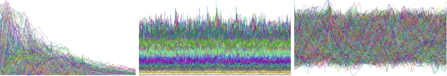
(a) earthquake data set (b) climate data set (c) vortex data set

Fig. 2. The importance curves of three time-varying data sets. The three data sets are from (a) a simulation of the1994Northridge earthquake (599

time steps), (b) a climate simulation of sea temperature over100years (1200time steps), and (c) a pseudo-spectral simulation of vortex structures (90time steps). The horizontal and vertical axes are time step and importance value respectively. Random colors are assigned to importance curves. By observing (a)-(c), we can infer that they belong to regular, periodic, and turbulent time-varying data, respectively.

Fig. 1. Examples of sample time window in1D (left) and2D (right) with weights given. The sizes of time window are7and3×3respectively.

color space) can be used to set the weight for the corresponding joint histogram bin (the smaller the distance, the larger the weight). Storing precomputed joint feature-temporal histograms allows a quick update of importance values when the transfer function changes at runtime.

The question remaining is how to choose related blocks Y for data block X . For practical reasons such as storage overhead and calcula-tion efficiency, we only consider the same spatial block as X but in the neighboring time steps for Y . That is, only the time steps within a given window are chosen. Typically, the window is along the one-dimensional time axis and centered at the time step where X resides in. It could also be in two (or higher) dimensions if the data is periodic and consists of one (or more) known cycle. In this scenario, the time window also samples neighboring time steps in neighboring cycles.

We define the importance of a data block Xjat time step t as follows: AX_j,t=

M

∑

i=1

wi·H(Xj,t|Yj,i), (4)

where M is the size of the sample time window, Yj,iis the ith sample

data block and wiis its corresponding weight. Two examples of time

window are shown in Fig. 1. As we can see, wifalls off as Yj,imoves

away from Xj,t. Note that the normalized wiis used, i.e.,∑

M i=1wi=1.

Finally, the importance of a time step t is the summation of the importance values of all data blocks in t. Written in equation:

At=

N

∑

j=1

AXj,t, (5)

where N is the number of data blocks at time step t.

3.4 Importance Curve

Calculating the importance value of a data block in the joint feature-temporal space along time yields a vector. Putting such a vector in the two-dimensional importance-time plot gives us an importance curve showing how the importance value of the data block changes over time. For instance, a high importance value at a time step indicates that at that time step, the data block contains a large amount of information by itself (high entropy) and it conveys less common information with other neighboring blocks (low mutual information). Conversely, a low importance value indicates that either the data block contains a small amount of information by itself (low entropy) or it conveys more com-mon information with other neighboring blocks (high mutual infor-mation). Drawing the importance curve for the whole volume (using importance values for each time step) summarizes the overall temporal behavior of the time-varying data.

4 CLUSTERINGIMPORTANCECURVES

If we plot all the importance curves of data blocks for the whole volume, manifest patterns reveal their respective categories of time-varying data. Fig. 2 shows three representative examples. The earth-quake data set shows a rise-and-fall trend. The climate data set gives a fluctuating pattern with varying amplitudes. The vortex data set, how-ever, exhibits an intertwined arrangement of curves. Their temporal behaviors thus fall into the categories of regular, periodic, and turbu-lent time-varying data, respectively. It is clear that drawing all the importance curves of data blocks poses a (potential) problem of visual clutter. An interesting followup task is to cluster importance curves, which helps us better observe distinct temporal trends of importance curves and classify the underlying time-varying data.

4.1 Hybridk-Means Clustering

In this paper, we utilize a hybrid k-means clustering algorithm [7] for importance curves clustering. The most common form of the pop-ular k-means algorithm uses an iterative refinement heuristic called

Lloyd’s algorithm. Lloyd’s algorithm starts by partitioning the input

points/vectors into k initial sets, either at random or using some heuris-tic data. Then, the algorithm calculates the centroid of each set and constructs a new partition by associating each point with its closest centroid. The centroids are recalculated for the new clusters, and the algorithm repeats until some convergence condition is met.

Although it converges very quickly, Lloyd’s algorithm can get stuck in local minima that are far from the optimal. For this reason we also consider heuristics based on local search, in which centroids are swapped in and out of an existing solution randomly (i.e., removing some centroids and replacing them with other candidates). Such a swap is accepted if it decreases the average distortion (the distortion between a centroid and a point is defined as their squared Euclidean distance); otherwise it is ignored. The hybrid k-means clustering al-gorithm combines Lloyd’s alal-gorithm and local search by performing some number of swaps followed by some number of iterations of Lloyd’s algorithm. Furthermore, an approach similar to simulated an-nealing is included to avoid getting trapped in local minima.

The top row of Fig. 3 shows clustering results on the three data sets where we clustered all time steps simultaneously. That is, an entire importance curve is treated as a T -dimensional point for clustering, where T is the number of time steps in the data. The number of clusters is controlled by the user and can be adjusted interactively at runtime. The centroids of clusters reflect different categories of data: they are clearly distinguishable in terms of amplitude for the earthquake and climate data sets, but are twisted together for the vortex data set.

4.2 Clustering Granularity

As highlighted in boxes in Fig. 3, cluster centroids can get too close or cross each other, which are highly correlated with the nature of the data being clustered. In our case, such results generally can be improved by adjusting the granularity of input to the clustering algorithm. More specifically, we partition all time steps sequentially into a list of time segments and cluster each segment separately, followed by a step of cluster matching for the whole time sequence. We match clusters by

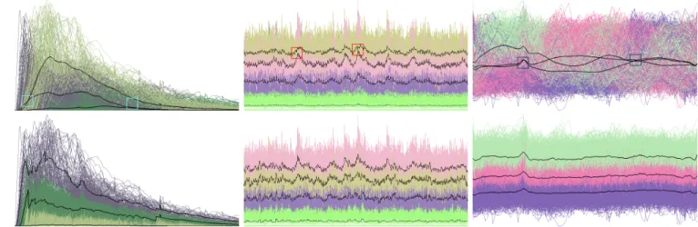
(a) earthquake data set (b) climate data set (c) vortex data set

Fig. 3. Clustering importance curves. Top row: results of simultaneous clustering all time steps. Bottom row: results of separate clustering time segments followed by cluster matching between segments. Using time segments helps avoid the centroids getting too close or crossing each other. The number of clusters in (a)-(c) is 3, 4, and 3 respectively. The centroids are displayed in black. In the bottom row, the number of time segments in (a)-(c) is50,120, and90respectively. The length of time segment is uniform in (b) and (c), but non-uniform in (a).

sorting the end points of the centroids in neighboring time segments and making one-to-one correspondence according to their orders. The number of segments is determined empirically. A larger number leads to a finer granularity of clustering along time. The length of each seg-ment can be either uniform (by default) or non-uniform (derived from the degree of temporal activity and accumulated importance values, see details in Section 5.4).

Our new clustering results are shown in the bottom row of Fig. 3. Using time segments helps reduce the overall average distortion as the centroids are pulled away from each other. Another advantage of this treatment is that unlike simultaneous clustering, a data block now may change its cluster membership throughout the time, which complies with the dynamic nature of time-varying data. As expected, changes in cluster membership happen more frequently for turbulent data than regular and periodic data, which is evident by comparing the images in Fig. 3.

5 IMPORTANCE-DRIVENVISUALIZATION

A visualization system can utilize importance values and importance curve clustering results in several different ways to, for example, iden-tify abnormal or unique features, enhance visualization, and lower both storage and computational costs.

5.1 Cluster Highlighting

Clustering importance curves of all data blocks in the volume gives us a new way to classify the underlying time-varying data. Examples in the bottom row of Fig. 3 show importance curves classified in terms of their amplitudes. A cluster of data blocks with higher amplitudes implies more dramatic changes of feature values; whereas a cluster of data blocks with lower amplitudes indicates less changes. Therefore, these classification results are very helpful for the users to isolate re-gions with various degrees of temporal activity for a clear observation. In the visualization, we ask the users to select one cluster at a time and the color and/or opacity transfer function can be adjusted accord-ingly to provide focus of attention to selected regions of interest. For instance, we can adjust the saturation of fragment colors in the shader depending on their class memberships. If a fragment does not belong to the chosen cluster, then we scale down its saturation as follows:

vec3 hsv = RGB2HSV(color.rgb); hsv.g *= alpha;

color.rgb = HSV2RGB(hsv.rgb);

wherecolor.rgbis the RGB color obtained from transfer function lookup,alpha∈(0,1)is the scaling factor, and functionsRGB2HSV

andHSV2RGBare for RGB and HSV color conversions. In practice, a

good focus+context effect can be generated with a low value (such as 0.1) foralpha. Such a solution can also be used to adjust the opacity

of fragment colors to provide contrast. With cluster highlighting, the users are able to purposefully focus on regions of interest and easily follow their evolutions over time.

5.2 Abnormality Detection

Our solution can be used to automatically detect abnormalities if the time-varying data contains such events. Following Eqn. 5, we know that all time steps may not be equally important in the data. Time steps with high importance values indicate when abnormalities oc-cur, since they correspond to data values fluctuating over the normal range. Similarly, we can further identify where abnormalities occur in those time steps. For each of the time steps with high importance values, additional markers can be placed to highlight a certain number of data blocks with the highest ranks of importance values (i.e., high-est degrees of temporal activity). In this manner, space-time abnormal events are highlighted for attention or alert.

5.3 Time Budget Allocation

Given a limited time budget for rendering or animation, we can allo-cate the time according to the importance values of time steps. The intuition is to spend more time on important time steps and less time on non-important ones. In this paper, we use the following equation to allocate the rendering or animation time to a time step t:

ωt=Ω· Aγt ∑T i=1A γ i , (6)

whereΩis the total time budget given, T is the number of time steps in the data, Atis the importance value of time step t, andγis the

expo-nential factor. In our experiment, typical values forγare in[0.5,2.0].

Note that for the case of rendering time allocation, the time allocated to each time step dictates the appropriate sampling spacing that should be used in rendering.

When only a limited amount of time budgetΩis given for render-ing or animation, our time allocation solution is most effective for a long sequence of data with varying importance values. For the case of rendering time allocation, more important time steps are rendered in higher quality and less important time steps are rendered in lower quality. Such an importance-driven rendering can be utilized in time-critical visualization. If necessary, a finer grain, block-wise rendering time breakdown could be sought in a similar fashion. For the case of animation time allocation, more important time steps are slowed down and less important time steps are speeded up. Therefore, due attention and ignorance are enforced.

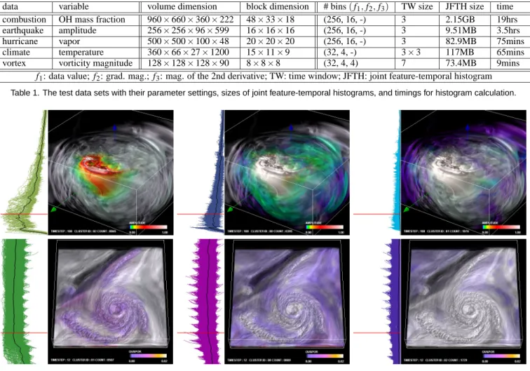
data variable volume dimension block dimension # bins(f1,f2,f3) TW size JFTH size time

combustion OH mass fraction 960×660×360×222 48×33×18 (256, 16, -) 3 2.15GB 19hrs earthquake amplitude 256×256×96×599 16×16×16 (256, 16, -) 3 9.51MB 3.5hrs hurricane vapor 500×500×100×48 20×20×20 (256, 16, -) 3 82.9MB 75mins climate temperature 360×66×27×1200 15×11×9 (32, 4, -) 3×3 117MB 65mins vortex vorticity magnitude 128×128×128×90 8×8×8 (32, 4, 4) 7 73.4MB 9mins

f1: data value; f2: grad. mag.; f3: mag. of the 2nd derivative; TW: time window; JFTH: joint feature-temporal histogram Table 1. The test data sets with their parameter settings, sizes of joint feature-temporal histograms, and timings for histogram calculation.

Fig. 4. Cluster highlighting. Top row: the earthquake data set. Bottom row: the hurricane data set. Left to right: clusters with high, medium, and low importance values. Clusters at the same time step (indicated by the red lines in their importance curves) are shown. Selected clusters are highlighted with high saturated colors while the rest of data are rendered with low saturated colors for the context.

5.4 Time Step Selection

Another interesting but often overlooked issue for time-varying data visualization is the selection of time steps from a long time sequence. When running a scientific simulation, scientists can adjust parameters to easily dump hundreds or thousands of time steps. Due to practi-cal reasons such as storage constraint and processing efficiency, they may only select a subset of time steps for analysis and visualization. The most common way of time step selection is to pick time steps uniformly from the time sequence (e.g., pick every kth time step). Al-though convenient, uniform selection of time steps may not be the ideal choice since the temporal behavior of the time-varying data could be quite uneven throughout the time.

For such type of data, we propose an algorithm to select time steps based on importance values: we start with selecting the first time step. Then, we partition the rest of time steps into(K−1)segments with near equal accumulated importance values Atin each segment, where K is the number of time steps to be selected. Finally, from each

seg-ment, we pick one time step:

t=argmax τ H(τ|t

0₎

, (7)

where t0 is the previously selected time step. Assuming a Markov sequence model for the time-varying data (i.e., any time step t is de-pendent on time step t−1, but independent of older time steps), the heuristic of our algorithm is to maximize the joint entropy of the se-lected time steps.

Animating the selected time steps gives a visual summary of the time-varying data. When a proper number of time steps are selected, such an animation conveys the important aspects of the data. More-over, the selected time steps can be considered as a representative set

of the original time sequence. Therefore, they can be used for further data analysis and visualization, such as feature extraction and time-varying transfer function specification, in a more efficient manner.

6 RESULTS

The test data sets and their variables we used in our experiments are listed in Table 1. All five floating-point data sets are from scientific simulations. The combustion simulation was conducted by scientists at Sandia National Laboratories (SNL) in order to understand the dy-namic mechanisms of combustion process. The earthquake simula-tion models the 3D seismic wave propagasimula-tion of the 1994 Northridge earthquake. The hurricane data set is from the National Center for Atmospheric Research (NCAR) and made available through the IEEE Visualization 2004 Contest. The simulation models Hurricane Isabel, a strong hurricane in the west Atlantic region in September 2003. The climate data set was provided by scientists at the National Oceanic and Atmospheric Administration (NOAA). The equatorial climate simula-tion covers 20◦S to 20◦N over a period of 100 years (one time step of data per month). Finally, the vortex data set has been widely used in feature extraction and tracking. The data is from a pseudo-spectral simulation of vortex structures.

Table 1 also lists the block dimension, the number of bins for fea-ture components, and the size of sample time window. With these settings, the size of joint histograms ranges from less than 1% (earth-quake data set) to about 10% (vortex data set) of the original size of data. All calculations were done using a 2.33GHz Intel Xeon

proces-sor. Note that the time to compute joint feature-temporal histograms dominates the total time for importance values calculation. The time for histogram calculation increases significantly as the size of data set

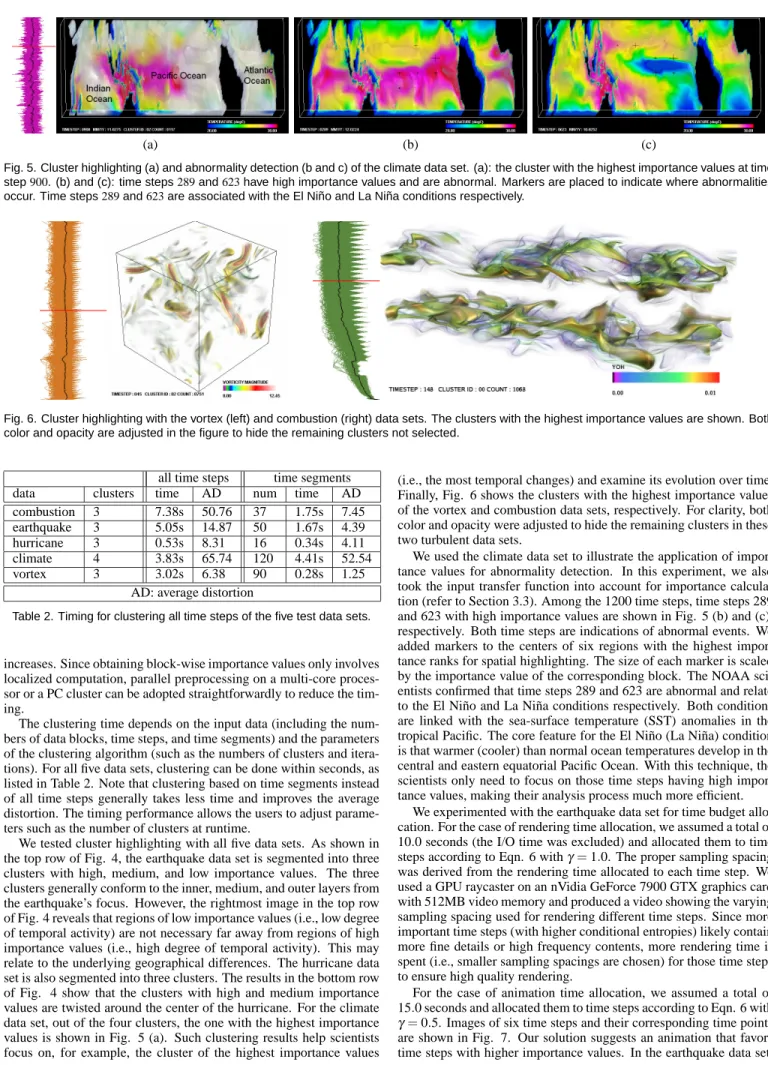
(a) (b) (c)

Fig. 5. Cluster highlighting (a) and abnormality detection (b and c) of the climate data set. (a): the cluster with the highest importance values at time step900. (b) and (c): time steps289and623have high importance values and are abnormal. Markers are placed to indicate where abnormalities occur. Time steps289and623are associated with the El Ni ˜no and La Ni ˜na conditions respectively.

Fig. 6. Cluster highlighting with the vortex (left) and combustion (right) data sets. The clusters with the highest importance values are shown. Both color and opacity are adjusted in the figure to hide the remaining clusters not selected.

all time steps time segments data clusters time AD num time AD combustion 3 7.38s 50.76 37 1.75s 7.45 earthquake 3 5.05s 14.87 50 1.67s 4.39 hurricane 3 0.53s 8.31 16 0.34s 4.11 climate 4 3.83s 65.74 120 4.41s 52.54 vortex 3 3.02s 6.38 90 0.28s 1.25

AD: average distortion

Table 2. Timing for clustering all time steps of the five test data sets.

increases. Since obtaining block-wise importance values only involves localized computation, parallel preprocessing on a multi-core proces-sor or a PC cluster can be adopted straightforwardly to reduce the tim-ing.

The clustering time depends on the input data (including the num-bers of data blocks, time steps, and time segments) and the parameters of the clustering algorithm (such as the numbers of clusters and itera-tions). For all five data sets, clustering can be done within seconds, as listed in Table 2. Note that clustering based on time segments instead of all time steps generally takes less time and improves the average distortion. The timing performance allows the users to adjust parame-ters such as the number of clusparame-ters at runtime.

We tested cluster highlighting with all five data sets. As shown in the top row of Fig. 4, the earthquake data set is segmented into three clusters with high, medium, and low importance values. The three clusters generally conform to the inner, medium, and outer layers from the earthquake’s focus. However, the rightmost image in the top row of Fig. 4 reveals that regions of low importance values (i.e., low degree of temporal activity) are not necessary far away from regions of high importance values (i.e., high degree of temporal activity). This may relate to the underlying geographical differences. The hurricane data set is also segmented into three clusters. The results in the bottom row of Fig. 4 show that the clusters with high and medium importance values are twisted around the center of the hurricane. For the climate data set, out of the four clusters, the one with the highest importance values is shown in Fig. 5 (a). Such clustering results help scientists focus on, for example, the cluster of the highest importance values

(i.e., the most temporal changes) and examine its evolution over time. Finally, Fig. 6 shows the clusters with the highest importance values of the vortex and combustion data sets, respectively. For clarity, both color and opacity were adjusted to hide the remaining clusters in these two turbulent data sets.

We used the climate data set to illustrate the application of impor-tance values for abnormality detection. In this experiment, we also took the input transfer function into account for importance calcula-tion (refer to Seccalcula-tion 3.3). Among the 1200 time steps, time steps 289 and 623 with high importance values are shown in Fig. 5 (b) and (c), respectively. Both time steps are indications of abnormal events. We added markers to the centers of six regions with the highest impor-tance ranks for spatial highlighting. The size of each marker is scaled by the importance value of the corresponding block. The NOAA sci-entists confirmed that time steps 289 and 623 are abnormal and relate to the El Ni˜no and La Ni˜na conditions respectively. Both conditions are linked with the sea-surface temperature (SST) anomalies in the tropical Pacific. The core feature for the El Ni˜no (La Ni˜na) condition is that warmer (cooler) than normal ocean temperatures develop in the central and eastern equatorial Pacific Ocean. With this technique, the scientists only need to focus on those time steps having high impor-tance values, making their analysis process much more efficient.

We experimented with the earthquake data set for time budget allo-cation. For the case of rendering time allocation, we assumed a total of 10.0 seconds (the I/O time was excluded) and allocated them to time

steps according to Eqn. 6 withγ=1.0. The proper sampling spacing

was derived from the rendering time allocated to each time step. We used a GPU raycaster on an nVidia GeForce 7900 GTX graphics card with 512MB video memory and produced a video showing the varying sampling spacing used for rendering different time steps. Since more important time steps (with higher conditional entropies) likely contain more fine details or high frequency contents, more rendering time is spent (i.e., smaller sampling spacings are chosen) for those time steps to ensure high quality rendering.

For the case of animation time allocation, we assumed a total of 15.0 seconds and allocated them to time steps according to Eqn. 6 with γ=0.5. Images of six time steps and their corresponding time points

are shown in Fig. 7. Our solution suggests an animation that favors time steps with higher importance values. In the earthquake data set,

Fig. 7. Animation time allocation with the 599 time steps earthquake data set. Left to right: six time steps correspond to six tick marks from left to right on a linear animation timeline. The statistics show that the first300time steps are given11.6seconds, leaving3.4seconds for the rest of time

steps. Our time allocation favors (i.e., gives more time to) time steps with higher importance values.

Fig. 8. Time step selection with the earthquake data set. 50of the599

time steps are selected (shown with blue dots on the importance curve). The goal is to maximize the joint entropy of the selected time steps.

they correspond to time steps (71 to 235) when seismic waves of high amplitude travel just under the Earth’s surface and make most of the destruction. The accompanying video demonstrates an importance-driven animation of the time sequence. Note that such a permutation of animation time is subjective and could be interpreted differently. Thus, the viewers should be advised of the context in advance. To provide an orientation for the viewers, we also showed a progress bar in the accompanying video indicating the varying playback speed.

Fig. 8 shows our time step selection results for the earthquake data set. We selected 50 time steps from the 599 time steps. Compared with uniform time step selection, our importance-based selection scheme yields a sequence of time steps with a much higher joint entropy of 14750.6, which is almost twice as the uniform selection of 7681.1.

We also include a video to compare the time steps selected by the uniform-based and our importance-based selection methods.

7 DISCUSSION

Viola et al. [16] introduced the idea of importance-driven volume ren-dering for automatic focus and context display of volume data. They assumed the objects within a volume are pre-segmented and each ob-ject is assigned an importance value by the users. Obob-ject importance is used to encode visibility priority for guiding importance-driven volume rendering. Our work targets time-varying scientific simula-tion data where no clear definisimula-tions of objects as those in medical or anatomical data are given. Unlike previous importance-driven ren-dering methods that require (discrete) volume segmentation or critical points calculation beforehand, our method uses the feature-temporal space for importance curve calculations and the subsequent clustering allows classifying regions of different degrees of temporal activity.

7.1 Parameter Choices

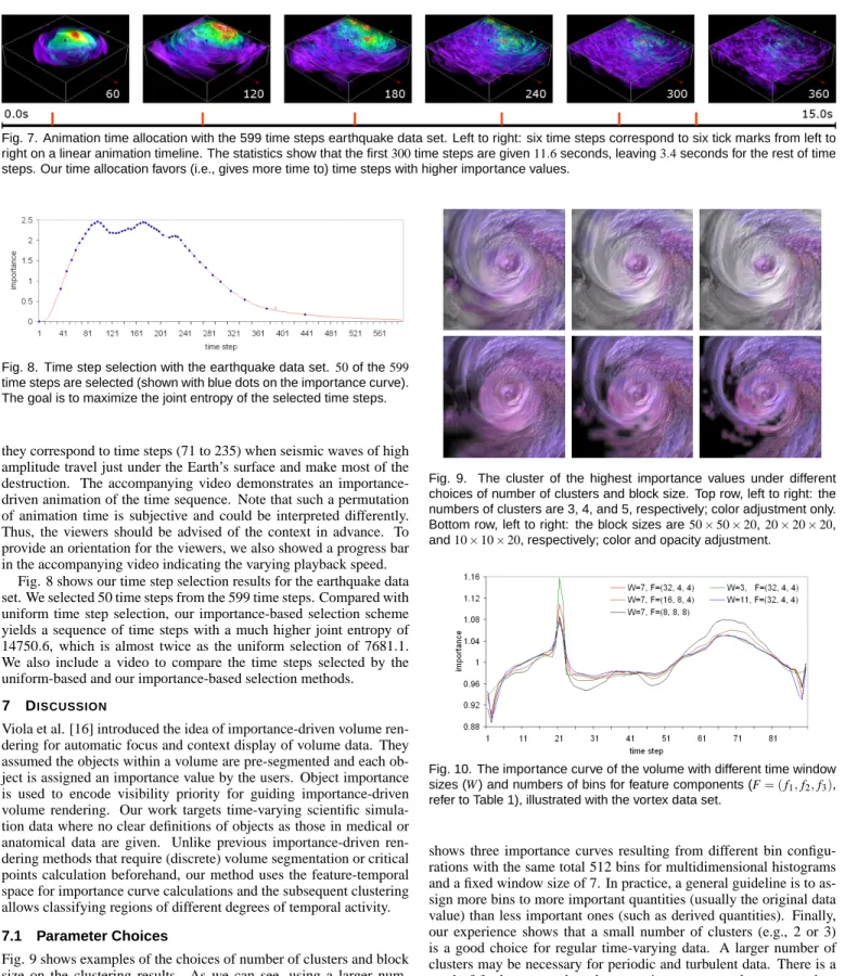
Fig. 9 shows examples of the choices of number of clusters and block size on the clustering results. As we can see, using a larger num-ber of clusters or a smaller block size leads to finer clustering results and thus distinguishes smaller features better. The overall hurricane structure is still captured when a larger block size is used. Note that the artifact along block boundaries becomes apparent when both color and opacity are adjusted. Our experiments show that the overall trend of importance curve is not sensitive to the size of time window chosen. Such an example is shown in Fig. 10. This justifies that sampling of time steps within a small local neighborhood suffices for importance evaluation. On the other hand, the numbers of bins selected for feature components have an influence on the importance curve. Fig. 10 also

Fig. 9. The cluster of the highest importance values under different choices of number of clusters and block size. Top row, left to right: the numbers of clusters are 3, 4, and 5, respectively; color adjustment only. Bottom row, left to right: the block sizes are50×50×20,20×20×20, and10×10×20, respectively; color and opacity adjustment.

Fig. 10. The importance curve of the volume with different time window sizes (W) and numbers of bins for feature components (F= (f1,f2,f3),

refer to Table 1), illustrated with the vortex data set.

shows three importance curves resulting from different bin configu-rations with the same total 512 bins for multidimensional histograms and a fixed window size of 7. In practice, a general guideline is to as-sign more bins to more important quantities (usually the original data value) than less important ones (such as derived quantities). Finally, our experience shows that a small number of clusters (e.g., 2 or 3) is a good choice for regular time-varying data. A larger number of clusters may be necessary for periodic and turbulent data. There is a need of further research and automation to suggest how many clus-ters to choose depending on the characteristics and actual content of the time-varying data. The number of clusters may also vary through different stages of the temporal activity. As for the choice of number of time segments, we suggest to use a large number for turbulent data sets in order to generate good clustering results. Regular and periodic data sets, however, are less influenced by this parameter value change.

7.2 Importance vs. Difference

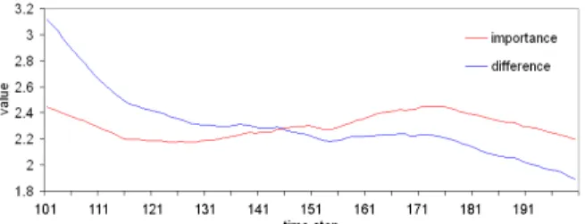
Temporal difference between time steps can be straightforwardly cal-culated by accumulating voxel-wise value differences. Our importance

Fig. 11. The contrast between our importance measure and temporal difference with the earthquake data set, time steps101to200.

measure is different from temporal difference in the following ways: First, our measure is based on the statistics of data blocks instead of separate values of individual voxels. Second, we use a multidimen-sional feature space to capture the changes of data from multiple per-spectives. Third, temporal difference only records absolute voxel dif-ferences between time steps. Our measure is based on the calculation of conditional entropy between time steps and is able to find more gen-eral correlations. For example, Fig. 11 shows the difference between our importance measure and temporal difference on the earthquake data set. It can be seen that while temporal difference shows an overall decreasing trend throughout the 100 time steps, our importance curve shows a different increasing trend between time steps 115 and 171.

7.3 Limitations

Our approach is based on the statistics of data blocks in the first place. The following clustering step also operates on data blocks. Therefore, we are only able to classify data in the block level. Reducing the block size could help refine classification results, but at the expense of in-creasing the size of joint histograms and affecting the efficiency of our approach. In the extreme case, if a block reduces to a voxel, then we lose the meaning of using this statistical approach. Note that this issue would be less of a concern as the size of data keeps increasing and the ratio between the data size and block size scales up. For very large data sets (such as 20483), a block-wise approach could be imperative from the efficiency point of view. Moreover, the k-means clustering algorithm uses a Gaussian assumption about the space of importance curves. The algorithm does not reveal how well a block fits into a given cluster. Further error visualization techniques can be sought to show importance curve clusters with more information.

7.4 Extensions

Several extensions can be made to improve our approach. First, the volume data can be partitioned into non-uniform data blocks accord-ing to the local data complexity. Such an adaptive scheme is expected to improve clustering results. Second, so far we only consider the same data block over time for importance analysis. It would be inter-esting to also take into account spatial neighboring data blocks. Third, our current method does not assume prior knowledge about the data. However, domain knowledge from scientists can be incorporated for a better importance analysis. For example, data ranges of interest can be utilized in the histogram construction. Fourth, besides what we have experimented, other domain-specific derivatives or quantities (such as different scalar variables or vector fields) can be used to augment the feature space. Finally, as the dimension of feature vector increases, a tradeoff between effectiveness and efficiency needs to be made for the number of bins used for each of its components. To avoid the “curse of dimensionality”, principal component analysis (PCA) or multidimen-sional scaling (MDS) can be applied for dimension reduction. These extensions would lead to a more effective derivation of importance values tailored to the scientists’ need.

8 CONCLUSION

In this paper, we introduce an approach to characterize the dynamic temporal behaviors exhibited by time-varying volume data. We de-rive an importance measure for each spatial block in the joint feature-temporal space of the data. Our approach is general in the sense that

it encompasses all three categories of time-varying data (regular, peri-odic, and turbulent). In a quantitative manner, we show that different spatial blocks have varying importance values over time and different time steps may not be equally important either. We show that there are several interesting and more cost-effective ways to visualize and un-derstand large time-varying volume data by utilizing their importance measures. Our importance analysis and visualization techniques thus provide a new direction to unveil and express the dynamic features of time-varying data.

ACKNOWLEDGEMENTS

This research was supported in part by the National Science Foun-dation through grants CCF-0634913, CNS- 0551727, OCI-0325934, OCI-0749227, and OCI-0749217, and the Department of Energy through the SciDAC program with Agreement No. DE-FC02-06ER25777, DE-FG02-08ER54956, and DE-FG02-05ER54817. We thank Jacqueline H. Chen and Andrew Wittenberg for providing the combustion and climate data sets, respectively. We also thank the re-viewers for their constructive comments.

REFERENCES

[1] H. Akiba, N. Fout, and K.-L. Ma. Simultaneous Classification of Time-Varying Volume Data Based on the Time Histogram. In Proc. of EuroVis ’06, pages 171–178, 2006.

[2] T. M. Cover and J. A. Thomas. Elements of Information Theory (2nd Edition). Wiley-Interscience, 2006.

[3] Z. Fang, T. M¨oller, G. Hamarneh, and A. Celler. Visualization and Ex-ploration of Time-Varying Medical Image Data Sets. In Proc. of Graphic Interface ’07, pages 281–288, 2007.

[4] S. Guthe and W. Straßer. Real-Time Decompression and Visualization of Animated Volume Data. In Proc. of IEEE Visualization ’02, pages 349–356, 2002.

[5] H. J¨anicke, A. Wiebel, G. Scheuermann, and W. Kollmann. Multifield Visualization Using Local Statistical Complexity. IEEE Trans. on Visu-alization and Computer Graphics, 13(6):1384–1391, 2007.

[6] T. J. Jankun-Kelly and K.-L. Ma. A Study of Transfer Function Gen-eration for Time-Varying Volume Data. In Proc. of Volume Graphics Workshop ’01, pages 51–68, 2001.

[7] T. Kanungo, D. M. Mount, N. S. Netanyahu, C. D. Piatko, R. Silverman, and A. Y. Wu. A Local Search Approximation Algorithm for k-Means Clustering. In Proc. of ACM Symposium on Computational Geometry ’02, pages 10–18, 2002.

[8] G. L. Kindlmann and J. W. Durkin. Semi-Automatic Generation of Trans-fer Functions for Direct Volume Rendering. In Proc. of IEEE Symposium on Volume Visualization ’98, pages 79–86, 1998.

[9] E. B. Lum, K.-L. Ma, and J. Clyne. A Hardware-Assisted Scalable So-lution for Interactive Volume Rendering of Time-Varying Data. IEEE Trans. on Visualization and Computer Graphics, 8(3):286–301, 2002. [10] G. Pass and R. Zabih. Comparing Images Using Joint Histograms.

Mul-timedia Systems, 7(3):234–240, 1999.

[11] H. Pfister, W. E. Lorensen, C. L. Bajaj, G. L. Kindlmann, W. J. Schroeder, L. S. Avila, K. Martin, R. Machiraju, and J. Lee. The Transfer Func-tion Bake-Off. IEEE Computer Graphics and ApplicaFunc-tions, 21(3):16–22, 2001.

[12] J. P. W. Pluim, J. B. A. Maintz, and M. A. Viergever. Mutual-Information-Based Registration of Medical Images: A Survey. IEEE Trans. on Medi-cal Imaging, 22(8):986–1004, 2003.

[13] H.-W. Shen, L.-J. Chiang, and K.-L. Ma. A Fast Volume Rendering Al-gorithm for Time-Varying Fields Using a Time-Space Partitioning (TSP) Tree. In Proc. of IEEE Visualization ’99, pages 371–377, 1999. [14] H.-W. Shen and C. R. Johnson. Differential Volume Rendering: A Fast

Volume Visualization Technique for Flow Animation. In Proc. of IEEE Visualization ’94, pages 180–187, 1994.

[15] I. Viola, M. Feixas, M. Sbert, and M. E. Gr¨oller. Importance-Driven Fo-cus of Attention. IEEE Trans. on Visualization and Computer Graphics, 12(5):933–940, 2006.

[16] I. Viola, A. Kanitsar, and M. E. Gr¨oller. Importance-Driven Volume Ren-dering. In Proc. of IEEE Visualization ’04, pages 139–145, 2004. [17] R. Westermann. Compression Domain Rendering of Time-Resolved

Vol-ume Data. In Proc. of IEEE Visualization ’95, pages 168–175, 1995. [18] J. Woodring, C. Wang, and H.-W. Shen. High Dimensional Direct

Ren-dering of Time-Varying Volumetric Data. In Proc. of IEEE Visualization ’03, pages 417–424, 2003.