PDXScholar
PDXScholar
TREC Theses and Dissertations Transportation Research and Education Center (TREC)
2019
Social Equity in Transit Service: Toward Social and
Social Equity in Transit Service: Toward Social and
Environmental Justice in Transportation
Environmental Justice in Transportation
Torrey Lyons
University of Utah
Follow this and additional works at: https://pdxscholar.library.pdx.edu/trec_etds
Part of the Transportation Commons, Urban Studies Commons, and the Urban Studies and Planning Commons
Let us know how access to this document benefits you.
Recommended Citation Recommended Citation
Lyons, Torrey, "Social Equity in Transit Service: Toward Social and Environmental Justice in Transportation" (2019). TREC Theses and Dissertations. 1.
https://pdxscholar.library.pdx.edu/trec_etds/1
This Dissertation is brought to you for free and open access. It has been accepted for inclusion in TREC Theses and Dissertations by an authorized administrator of PDXScholar. For more information, please contact
Social Equity in Transit
Service
: Toward social
and environmental justice in transportation
Aug
2019
Torrey Lyons, Ph.D.
SOCIAL EQUITY IN TRANSIT SERVICE:
TOWARD SOCIAL AND ENVIRONMENTAL
JUSTICE IN TRANSPORTATION
By
Torrey James Lyons
A dissertation submitted to the faculty of the University of Utah in partial fulfillment of the degree of
Doctor of Philosophy
Department of City and Metropolitan Planning The University of Utah
Copyright © Torrey James Lyons 2019 All Rights Reserved
ABSTRACT
This dissertation explores social equity as it applies to public transportation. Transit has long been considered a tool to alleviate inequity by limiting the effects of spatial mismatch and providing access to opportunity to disadvantaged populations. This theory, however, has not been adequately proven empirically. The first chapter of this dissertation tests the theory that spatial mismatch is moderated by quality transit service. We do this by taking a cross section of the largest urban areas in the United States and applying structural equation modeling to identify relationships between exogenous and endogenous factors. We find that higher quality transit service and compactness are associated with lower levels of unemployment, poverty, and income inequality. The second chapter of this dissertation outlines the development of a novel index for objectively measuring social equity in transit service. This methodology improves upon previous efforts to quantify equity in transit by using emerging techniques in geographic information systems (GIS) software and by incorporating a comprehensive set of index components. The third chapter explores how transit agencies plan for providing equitable transit service. We interview transit agency planners to understand the way that agencies consider equity, to determine how equity considerations are shaped by agency and federal policy, and we compare these considerations to themes in the academic literature. We find that while academic efforts have focused primarily on accessibility as the most important facet of equity in transit service, transit agency planners think of equity in a more wholistic manner. The accessibility framework, as we describe it here, is a less nuanced way to think of and plan for equity than how transit agencies are currently operating. Additionally, we attribute part of agencies’ more
comprehensive construction of equity to Title VI of the Equal Rights Act of 1964. This legal framework for planning for equity is ubiquitously criticized in the academic literature for being inadequate at measuring the accessibility effects of changes to transit service. Although these claims have merit, the framework considers equity in a way that goes beyond just measuring accessibility and therefore contributes to a broader lens through which transit agencies think about and plan for equity.
CONTENTS
ABSTRACT ... iv
LIST OF TABLES ... ix
LIST OF FIGURES ... x
Chapters
1 INTRODUCTION ... 1
2 THE EFFECTS OF TRANSIT AND COMPACTNESS ON REGIONAL
ECONOMIC OUTCOMES ... 15
ABSTRACT ... 6
2.1 INTRODUCTION ... 7
2.2 LITERATURE REVIEW ... 9
2.3 METHODS ... 15
2.4 RESULTS ... 24
2.5 CONCLUSION ... 36
2.6 REFERENCES ... 41
3 TRANSIT ECONOMIC EQUITY INDEX: DEVELOPING A COMPREHENSIVE
MEASURE OF TRANSIT SERVICE EQUITY ... 45
ABSTRACT: ...46
3.1 INTRODUCTION: ...47
3.2 LITERATURE REVIEW: ...49
3.3 METHODOLOGY: ...53
3.4 RESULTS: ...67
3.5 DISCUSSION ...74
3.6 LIMITATIONS ...77
3.7 REFERENCES ...80
4 BEYOND TITLE VI: HOW TRANSIT AGENCIES PLAN FOR EQUITY ...83
ABSTRACT ...84
4.2 CONCEPTUAL FRAMEWORK AND RESEARCH DESIGN ...94
4.3 DATA COLLECTION AND ANALYSIS ... 97
4.4 FINDINGS ...102
4.5 DISCUSSION ...116
4.6 REFERENCES ...118
LIST OF TABLES
Tables
2.1 Literature-Informed Variable Selection ………16
2.2 Variables and Data Sources ………...17
2.3 PCA Extraction ………..20
2.4 PCA Variance Explained ………21
2.5 Descriptive Statistics of Final Model Variables ……….22
2.6 Inequality Model SEM Path Coefficient Estimates ………26
2.7 Inequality Model Covariance Estimates ……….27
2.8 Inequality Model Direct, Indirect, and Total Effects ………..27
2.9 Poverty Model SEM Path Coefficient Estimates ………31
2.10 Unemployment and Poverty Model Covariance Estimates ………..32
2.11 Poverty Model Direct, Indirect, and Total Effects ………32
3.1 Unemployment and Poverty Model Covariance Estimates ………55
3.2 Case Study Select Descriptive Statistics ……….57
LIST OF FIGURES
Figures
2.1 Great Gatsby Curve ………12
2.2 Inequality Model SEM Path Diagram ………25
2.3 Total Effects on Income Inequality ………29
2.4 Unemployment and Poverty Model SEM Path Diagram………30
2.5 Total Effects on Unemployment ……….33
2.6 Total Effects on Poverty ………..34
3.1 Case Selection Based on Transit ……….56
3.2 Disadvantage Index Seattle ……….60
3.3 Average 8 AM Peak Disadvantaged Work Trip Travel Speeds ……….67
3.4 Transit Service Convenience Score ………68
3.5 Non-Peak Hour Service Score ………69
3.6 System Access Scores ……….70
3.7 Transit Economic Equity Index Scores ………...72
3.8 All Index Component Scores ………..73
4.1 Conceptual framework of planning for equity in transit ……….94
CHAPTER 1: INTRODUCTION
Social and environmental justice have been a concern in transportation planning for almost as long as these terms were in the national policy lexicon. Social equity can be defined as an equitable distribution of goods, services, rights, and opportunities (Deka, 2004). Equity is often categorized as either vertical or horizontal; the former describing a scenario in which all people are treated the same, and the latter in which intentionally disparate impacts of policy are designed to advance traditionally marginalized groups. Title VI of the Civil Rights Act of 1964 introduced the concept of environmental justice to transportation by directing agencies to “demolish the barriers to full participation faced by minorities.” In this act, Congress further stipulates that “[n]o person in the United States shall, on the ground of race, color, or national origin, be excluded from participation in, be denied the benefits of, or be subjected to
discrimination under any program or activity receiving Federal financial assistance.” (Colopy, 1994) Given the heavy subsidization of US transportation systems, it is not surprising that equity considerations have been mandated for some time. Equity analyses are required of transit
agencies and metropolitan planning organizations (MPOs), although the methods that they use are rudimentary at best (Karner & Niemeier, 2013; Sanchez & Wolf, 2005)
The topic of income inequality has recently come to the forefront of political discourse (Deininger & Squire, 1996; Atkinson, 1983; Glomm & Ravikumar, 1992; Ngamba, Panagioti & Armitage, 2017; Jacobs & Dirlam, 2016; Hero, 2016). Although it was posited by Kuznets (1955) that income inequality would decline with the progression of the development of a nation, the United States has not followed his proposed theoretical trajectory. In fact, the recent decades
have been characterized by a decline in the share of wealth controlled by the bottom 90% of American workers. (Corak, 2013) This is a troubling trend, and its causes must be examined.
Interestingly, it has been posited that the way that our cities are configured has had an influence on economic opportunity for marginalized populations in the US (Durlauf, 1996; Rey, 2004; Lessman, 2014.) Spatial mismatch is a theory that was first developed in 1968 by John Kain which highlights the geographic disparity of low skill jobs and the location of low skilled workers’ housing. The exodus of affluent white households to the suburbs after WWII
precipitated a change in the location of low-skilled service jobs from the city to the suburbs. The workers best suited for these jobs, however, were forced to remain in the city for the lack of affordable housing options in the newly minted suburbs. Kain attributed high unemployment rates and persistent poverty to spatial mismatch.
While those who have access to private vehicles appreciate an expansive roadway system, this luxury is not available to the most disadvantaged populations. Those without access to an automobile rely on transit for much of their transportation needs. These populations are considered “transit dependent” (Litman, 1996). Transit dependency describes an economic condition of being mostly reliant on transit to access one’s daily transport needs. This population depends on bus and rail networks to partake in even the most basic activities such as work, education, and even health care. Consequently, many argue that we must provide adequate public transit networks to increase access to daily needs for the most vulnerable and economically disadvantaged populations.
While automobile travel is greatly subsidized through low fuel prices, free access to high quality roads, purchasing incentives, free parking, uncompensated accident costs, and
Mallinckrodt, 2003; Ewing, 1997; Shoup, 2017; Beck, 2003; Delucchi, 1996; Edlin & Karaca-Mandic, 2006; Delucchi, 2000). Investment per rider is a term used by transit agencies to
quantify the dollar amount that it actually costs to take a passenger on an average length trip, and this number can far-exceed the normal cost of the fare (Litman, 2008). With such public
investment into the affordability of transit service, it should be established whether or not agencies are achieving their goals of improving accessibility to jobs and other daily needs of disadvantaged riders.
Some researchers have attempted to develop methodologies for measuring social equity in transit service. The focus thus far has been on the spatial component of transit service,
measuring accessibility for disadvantaged populations. A few studies have taken it a step further by including temporal elements as well. It is important to measure both time and space when considering the equity of transportation systems, as people interact with the built environment along a spectrum of these dimensions. There are two key shortcomings of the efforts of researchers thus far. The first of these is the exaggerated focus on the spatial aspect of transit equity. While transportation is ultimately about linking origins and destinations, there are many more facets of transit systems which either improve equity in transportation or limit it. This calls for a measure that is more comprehensive, including more aspects of transit service than just spatial and temporal elements. Second, the methodologies of previous studies are rigorous to a point of being inaccessible to the typical transit planner. What good is a methodology which can only be replicated by select researchers with a very specialized skill set? This highlights the need for a comprehensive, accessible methodology which can be widely applied to transit agencies around the country for the purpose of evaluating their efficacy in promoting social equity.
After constructing the improved methodology for measuring equity in transit service, we can then better understand how agencies are achieving equitable transit systems. We relate agency practices and policies to performance with respect to the index in order to determine what practical aspects of transit agencies lend themselves to equitable systems. We then investigate transit agencies with varying degrees of success in providing equitable systems to identify best practices. Finally, the index allows for an investigation of whether regions with equitable transit systems experience improved economic outcomes like lower levels of persistent poverty and unemployment. Determining whether there is an economic case for socially equitable transit service helps in determining whether additional public funding for the mode is warranted. These efforts are a novel contribution to the field and will provide insight into the important issue of social equity in transit.
CHAPTER 2:
THE EFFECTS OF TRANSIT AND
COMPACTNESS ON REGIONAL
ECONOMIC OUTCOMES
ABSTRACT
Kain’s theory of spatial mismatch states that the physical separation of people from their employment contributes to persistent unemployment and poverty. Transit has long been
considered a way to alleviate this issue by providing access to opportunity for disadvantaged populations. In this paper we test the theory that transit can act as a moderator on the relationship between spatial mismatch and unemployment and poverty. We find that transit does affect unemployment and poverty indirectly through its effect on compactness. This study is the first to find a relationship between transit and poverty using a national sample of large US regions. The findings give credence to transit supportive policies that seek to use transit as a lever to improve regional economic conditions and alleviate unemployment and poverty.
INTRODUCTION
In the late 1960s, Kain observed that the exodus of affluent white Americans to the suburbs was creating what he called the problem of spatial mismatch. Spatial mismatch describes the phenomenon wherein people and jobs are separated by space, making it harder for specific populations to access economic opportunities. Access to transportation, in theory, can act to moderate the effect of spatial mismatch on poverty and unemployment. Personal vehicles
effectively nullify the problem, as access to this mode allows commuters to travel great distances from their homes to workplaces in a relatively short amount of time. What about those who do not have access to personal vehicles? Transit, again theoretically, can help to extend the amount of opportunities for those without automobiles. The assumption that transit provides economic opportunity is a basic assumption in transportation planning practice and academia, but there has been limited empirical study of this premise to date. As Sanchez (2008) puts it, “The connection between transportation mobility and poverty is laden with untested assumptions,”
Updates to this work have found associations between poor public transit access and higher rates of unemployment and poverty (Kain & Meyer, 1970; Kasarda, 1983; Elwood, 1986; Ihlanfeldt, 1993; Sanchez, 1999; Sanchez, 2008). Many studies have examined the relationships between transportation investments in given areas and their corresponding impacts on regional economies. These studies associate lagged changes in economic variables to transportation investments or policies (Berechman, Ozmen, & Ozbay, 2006; Sanchez, 2008). A large-scale examination of how transportation variables interact with socioeconomic and
built-environmental determinants of unemployment and poverty is an effort that has not yet been undertaken in the urban planning literature. With this paper, we study how transit affects regional economic outcomes, unemployment and poverty. We do this using a cross-sectional study design of 113 US urbanized areas. We use structural equation modeling to determine if transit can act as a moderating factor on the relationship between spatial mismatch and unemployment and
LITERATURE REVIEW
SPATIAL MISMATCH
The above problems have been studied by economics scholars and are known to be caused by a variety of factors including wage stagnation, banking practices, public policy, and sprawling development patterns. (Reed, 1999; Dabla-Norris et al., 2015; Kaplan et al., 1996; Bakija et al., 2012; Ewing et al., 2016) However, there are only so many ways in which urban planners can attempt to tackle this problem. One way, as is posited in this dissertation, is through addressing yet another issue that has been suggested to influence intergenerational poverty: spatial mismatch.
Spatial mismatch is a theory that was first developed in 1968 by John Kain, which highlights the geographic disparity of low skill jobs and the location of low skilled workers’ housing. The exodus of affluent white households to the suburbs after WWII precipitated a change in the location of low-skilled service jobs from the city to the suburbs. The workers best suited for these jobs, however, were forced to remain in the city for the lack of affordable housing options in the newly minted suburbs. Kain attributed high unemployment rates and persistent poverty to spatial mismatch. The theory originally focused on inner city African American populations, but it has now expanded to incorporate all vulnerable populations around the world. They posit that it is the reformation of urban structure that has created the serious economic problems facing the most vulnerable populations (Wolf, 2007; Harper, Marcus & Moore, 2003; Moore, 2005; Horrell, Humphries & Voth, 2001).
Later on, transportation researchers began to refine the theory to incorporate the evolving expertise of the field. Cervero (1989) discovered that regional mobility is related to spatial mismatch. He went on to develop the concept of jobs-housing balance, which attempts to pinpoint a comfortable equilibrium of land uses that allows residents to easily access sufficient employment opportunity. In 2002, Cervero et al. further advanced the understanding of this relationship by linking transportation policy to the ability of individuals to find employment. This study used a rich longitudinal dataset which followed individuals that had been on welfare. Cervero et al. use the switch from welfare to work as an indicator of a sign of improvement of an individual’s economic situation. They find that car ownership and educational attainment were the strongest predictors of individuals’ ability to transition from welfare to work. This indicates a transportation system which is not properly providing opportunity for the most disadvantaged populations like those who do not have access to a private vehicle.
INCONME INEQUALITY AND INTERGENERATIONAL MOBIITY
Income inequality is an issue that has garnered a great deal of attention in the past few years. From the work of Chetty and other researchers to the political talking points of Sanders and Warren of the political left, we are increasingly more aware of the potential of this problem to continue to fragment our society.
One of the first researchers on the topic, Simon Kuznets (1955) claims that after the First World War, income distribution in the US and England was actually becoming more equitable. In the US, for example, the proportion of total income attributable to the lowest two quintiles rose from 13.5% in 1929 to 18% in 1950. Comparing this trend to today, we see much more
inauspicious figures. Although it was posited by Kuznets (1955) that income inequality would decline with the progression of the development of a nation, the United States has not followed his proposed theoretical trajectory. In fact, the recent decades have shown a decline in the share of wealth controlled by the bottom 90% of earners. (Corak, 2013) Just as disheartening are the findings of a recent OECD report which established the gap between the rich and poor to be at its highest level in the past 30 years. (Cingano, 2014) This report also determined that the
expanding gap has a significant impact on aggregate economic growth. Interestingly, Cingano demonstrates that it is not the elevation of the highest earners, which has the largest negative effect, but rather the depression of low-income households that harms the economy. Forster and Pellizzari (2000) suggest that this is a global trend, with no OECD nations experiencing
decreases in inequality.
A related topic of interest to urban researchers that is simply an extension of the issue of income inequality is intergenerational poverty. As compassionate observers of social issues, we are indeed troubled by the impoverished conditions of so many citizens. What is even more troubling, however, is when those impoverished households are unable to help lift their children out of similar circumstances, leaving them to lead a similar taxing existence. Corak (2013) finds that increasing polarization of income inequality leads to decreased intergenerational mobility. Intergenerational mobility is a concept that can be defined by a child’s likelihood of finding himself in a different income category than he was born into specifically from a lower category to a higher category. While Corak’s assertion is not uniformly supported by other economic scholars, it is an unsettling notion that warrants further examination. (Chetty, 2014; Bratberg et al., 2017; Landerso & Heckman, 2017; Blanden et al., 2013; Stoker & Ewing, 2014)
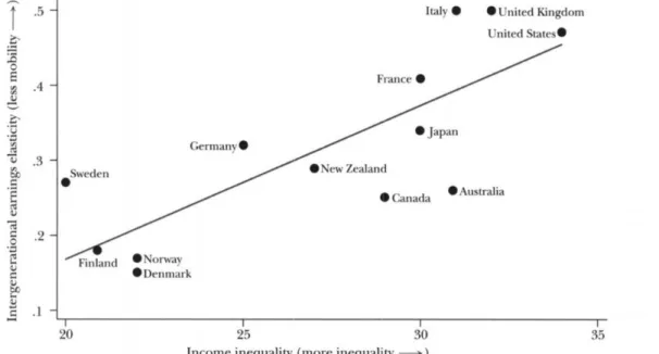
Corak (2013) introduces and interesting economic theory which he calls the Great Gatsby Curve. The Great Gatsby is a considered a cautionary tale which warns of the downfalls of excess and resistance to change. This important and effective visualization depicts OECD countries on a graph of income inequality and intergenerational mobility. Below, the Great Gatsby Curve shows the United States at the extreme of income inequality with a reciprocal inferiority in intergenerational mobility among the countries included in the graph.
FIGURE 2.1 Great Gatsby Curve
DETERMINANTS OF UNEMPLOYMENT AND POVERTY
The theory of spatial mismatch suggests that the separation in space between people and jobs leads to unemployment and poverty in disadvantaged populations. However, this certainly is not the only driver of economic outcomes for individuals, regions, or countries. Economists have
long studied the determinants of unemployment and poverty, but have traditionally looked at differences between nations, as this allows for the analysis of how national policies can affect economic outcomes. The determinants of regional economic outcomes are studied less, but those that have examined these relationships have reported similar findings. Demographic factors such as race and ethnicity, educational attainment, age, religion, and diversity have been aggregated to varying geographies and related to regional economic outcomes (Achia, Wagombe, & Khadioli, 2010; Moller et al., 2003; Rapusingha & Goetz, 2007; Filitztekin, 2008; Bardinger et al., 2002; Sanchez, 1999, Zenou, 2000). Economists and planners have also found that built-environmental factors such as employment density, population density, and distance to jobs affect
unemployment and poverty (Rapusingha & Goetz, 2007; Filitztekin, 2008; Bardinger et al., 2002; Sanchez, 1999, Zenou, 2000). Others have examined how labor force characteristics, household structure, public policy, and even transportation factors influence regional economic outcomes (Achia, Wagombe, & Khadioli, 2010; Pichaud, 2002; Moller et al., 2003; Rapusingha & Goetz, 2007; Filitztekin, 2008; Bardinger et al., 2002; Sanchez, 1999).
The best effort to date to relate transportation infrastructure with unemployment is Sanchez, 2007. In this study, Sanchez investigates the relationship between access to public transportation and labor force participation rates. Sanchez analyzes two case studies, comparing block groups and measuring a variety of demographic information for this geography. The author found that access to public transit was a good indicator of workforce participation in Portland, OR and Atlanta, GA. While this study provides some evidence that transit service provision can affect economic outcomes at the block group level, the findings of this study are limited in their generalizability due to the small sample of regions (Pichaud, 2002) and the smaller geographic level of analysis. This paper will build upon the findings of Sanchez (2007) by expanding the
sample to almost all large regions in the US, and analyzing economic outcomes at the regional level. Such an improvement also has the potential to strengthen the case for using transportation spending as an economic lever if it were to find that transit is, in fact, a determinant of regional economic outcomes.
METHODS
STUDY DESIGN
This study tests the hypothesis that a robust transit system can influence regional
economies. Kain (1955) posits that spatial mismatch leads to issues of persistent poverty and low intergenerational mobility. By relating transit service provision to income inequality and poverty, we can potentially verify the theory that transit service can function as a moderator on the
relationship between spatial mismatch and persistent poverty. This paper employs a cross-sectional study design using structural equation modeling on an enhanced database, combining built-environmental, socioeconomic, and transportation system variables. The addition of new variables brings the total number of regions in the database to 113.
DATA AND VARIABLES
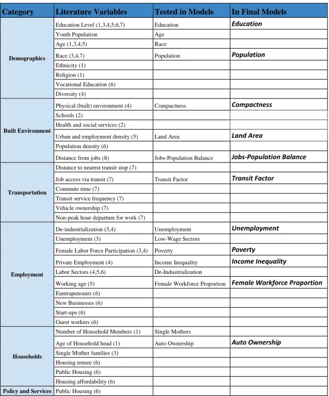
While we rely on the expertise of the authors and contributors to determine which transportation and built-environmental variables will best serve the purposes of the models, sociodemographic and economic factors needed to be more explicitly-informed by the literature. We performed an additional literature review of the determinants of regional unemployment and poverty to help decide which constructs would be operationalized, and how. Table 2.1 depicts
the determinants of unemployment and poverty as defined by the literature. We also highlight which variables we included in early model iterations as well as those persisting to final models.
TABLE 2.1 Literature-Informed Variable Selection
Category Literature Variables Tested in Models In Final Models
Demographics
Education Level (1,3,4,5,6,7) Education Education Youth Population Age
Age (1,3,4,5) Race
Race (3,4,7) Population Population
Ethnicity (1) Religion (1)
Vocational Education (6) Diversity (4)
Built Environment
Physical (built) environment (4) Compactness Compactness Schools (2)
Health and social services (2)
Urban and employment density (5) Land Area Land Area Population density (6)
Distance from jobs (8) Jobs-Population Balance Jobs-Population Balance
Transportation
Distance to nearest transit stop (7)
Job access via transit (7) Transit Factor Transit Factor Commute time (7)
Transit service frequency (7) Vehicle ownership (7)
Non-peak hour departure for work (7)
Employment
De-industrialization (3,4) Unemployment Unemployment Unemployment (3) Low-Wage Sectors
Female Labor Force Participation (3,4) Poverty Poverty
Private Employment (4) Income Inequality Income Inequality Labor Sectors (4,5,6) De-Industrialization
Working age (5) Female Workforce Proportion Female Workforce Proportion Euntrapenouirs (6)
New Businesses (6) Start-ups (6) Guest workers (6)
Households
Number of Household Members (1) Single Mothers
Age of Household head (1) Auto Ownership Auto Ownership Single Mother families (3)
Housing tenure (6) Public Housing (6) Housing affordability (6)
Schools (2)
Health and social services (2) Government Expenditure (4)
1: Achia, Wagombe, and Khadioli (2010) 4: Rapusingha & Goetz (2007) 7: Sanchez (1999) 2: Pichaud (2002) 5: Filitstekin (2008) 8: Zenou (2000) 3: Moller et al. (2003) 6: Bardinger & Url (2002)
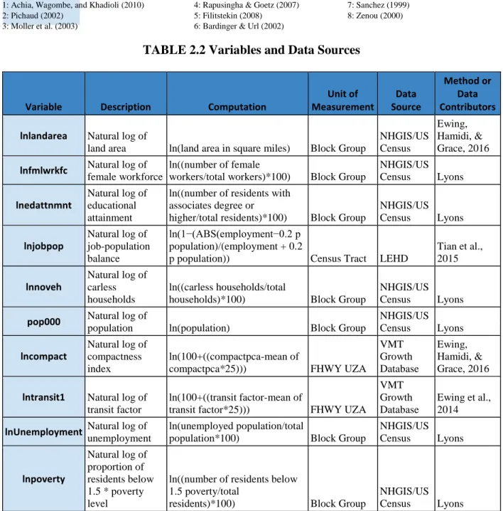
TABLE 2.2 Variables and Data Sources
Variable Description Computation
Unit of Measurement Data Source Method or Data Contributors lnlandarea Natural log of
land area ln(land area in square miles) Block Group
NHGIS/US Census Ewing, Hamidi, & Grace, 2016 lnfmlwrkfc Natural log of female workforce ln((number of female
workers/total workers)*100) Block Group
NHGIS/US Census Lyons lnedattnmnt Natural log of educational attainment
ln((number of residents with associates degree or
higher/total residents)*100) Block Group
NHGIS/US Census Lyons lnjobpop Natural log of job-population balance ln(1−(ABS(employment−0.2 p population)/(employment + 0.2
p population)) Census Tract LEHD
Tian et al., 2015 lnnoveh Natural log of carless households ln((carless households/total
households)*100) Block Group
NHGIS/US Census Lyons
pop000 Natural log of
population ln(population) Block Group
NHGIS/US Census Lyons lncompact Natural log of compactness index ln(100+((compactpca-mean of
compactpca*25))) FHWY UZA
VMT Growth Database Ewing, Hamidi, & Grace, 2016
lntransit1 Natural log of transit factor
ln(100+((transit factor-mean of
transit factor*25))) FHWY UZA
VMT Growth Database
Ewing et al., 2014
lnUnemployment Natural log of
unemployment
ln(unemployed population/total
population*100) Block Group
NHGIS/US Census Lyons lnpoverty Natural log of proportion of residents below 1.5 * poverty level
ln((number of residents below 1.5 poverty/total
residents)*100) Block Group
NHGIS/US Census Lyons
Many of the above variables, their computation, and sourcing do not demand further explanation. However, here we will discuss the computation of some of the variables, the decision to choose varying units of measurement, and the process of spatially apportioning data. The final unit of analysis was the Federal Highway Administration Urbanized Area. This
research is built partially on the efforts of previous work that has emerged from the colleagues at the University of Utah. Ewing, Hamidi, and others have worked to develop sprawl metrics that have been linked to urban phenomena like obesity, vehicle miles traveled, traffic safety, and congestion. They have created a rich database that was generated using GIS to measure many attributes of sprawl. Socioeconomic data gathered from IPUMS’ National Historical GIS (NHGIS) are measured at US Census geographies. The boundaries for Census geographies and those of FHWA UZAs differ, and therefore, spatial apportioning of NHGIS data was necessary. Below, Figure 2.1 depicts the dissimilarities between Census and FHWA geographies.
Figure 2.1 Census Tracts and FHWA Urbanized Area
The area highlighted in pink represents the Census urban area, and the area outlined in red represents the FHWA adjusted urbanized area. A reason for FHWA’s adjustments is to reduce the irregularity in Census designations for the purpose of improved transportation
planning. In order to use data measured at the Census geography within the UZA, first we must determine the smallest possible geography for the variables in question. Census block groups were used for most variables, except when a larger unit of analysis was the most prudent way to measure a construct. An example of a case where a larger unit of analysis was more appropriate is job-population balance. This is a construct that considers the availability of jobs within relatively close proximity to residents (Cervero & Duncan, 2006; Weitz, 2003; Stoker & Ewing, 2014). We assert that a block group, which is often considered the best analog to a neighborhood of census geographies is too small. A typical conceptualization of a neighborhood is small, and will often not contain any areas of meaningful employment. Thus, we measure job-population balance at a Census tract level, which is larger than a block group, but still small enough to reasonably apportion within the UZA boundary. Census tracts were also used as the unit of measurement for income inequality for the same reason.
We used spatial apportioning to assign data measured at smaller geographies (tracts and block groups) to the UZA. We intersected tracts and block groups with UZA’s and measured the proportion of the tract or block group that falls within the UZA boundary. That proportion was then used to assign the appropriate amount of data to the urbanized area. This process is known as simple area weighting, and is detailed in the below equation:
Where: Vt is the value in the target zone t; Vs is the population in source zone s; As is the area of source zone s; and Ats is the area of target zone t overlapping source zones. Two of the variables in the dataset are factors derived from principal component analysis. Principal component analysis (PCA) is a process wherein a researcher creates a new variable that represents the shared variation between multiple like variables. This allows the researcher to
create a more parsimonious model using only a single variable that explains the variation of multiple variables. This method was used by Ewing et al. in 2018 when they tested Newman and Kenworthy’s theory of density and automobile dependence. In order to more succinctly express the inverse of sprawl, they created an index which they called “compactness”. Their compactness variable was the product of a principle component analysis four factors including density, mixed-use, centering, and street network design. This measurement was taken directly from the dataset that Ewing et al. constructed, with the authors’ permission. Additionally, we used PCA to create a new “transit” factor. The transit factor represents the common variation in five variables that express different elements of transit service provision: route density; service frequency; total operating expenditure; fare price; and unlinked passenger trips per capita. Below, Tables 2.3 and 2.4 depict the extractions from each original transit service provision variable as well as the total variance explained by the new PCA variable.
TABLE 2.3 PCA Extraction
Communalities Initial Extraction lnfare 1.000 .709 rtden 1.000 .725 tfreq 1.000 .654 lntotalopexp 1.000 .854 UnlkdPasTripCap 1.000 .913
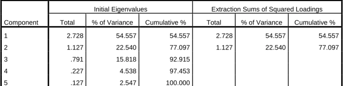
TABLE 2.4 PCA Variance Explained
Total Variance Explained
Component
Initial Eigenvalues Extraction Sums of Squared Loadings Total % of Variance Cumulative % Total % of Variance Cumulative % 1 2.728 54.557 54.557 2.728 54.557 54.557 2 1.127 22.540 77.097 1.127 22.540 77.097
3 .791 15.818 92.915
4 .227 4.538 97.453
5 .127 2.547 100.000
Extraction Method: Principal Component Analysis.
SPSS software produces a new variable that is an expression of the shared variance of the variables that are included in the PCA. We use just the first PCA variable as it alone explains the majority of the common variance of all component variables. Adding a second PCA variable would complicate the model theoretically with limited gains in explanatory value. This new variable is scaled to be normally distributed, have a mean of zero, and a standard deviation of one. In order to have the variable expressed in a way that is more intuitively interpretable, we transformed the resulting PCA variable to have a mean of 100 and a standard deviation of 25. Below, Table 2.5 includes descriptive statistics for all variables included in the final models. The variables described below are not log-transformed as they are in the models.
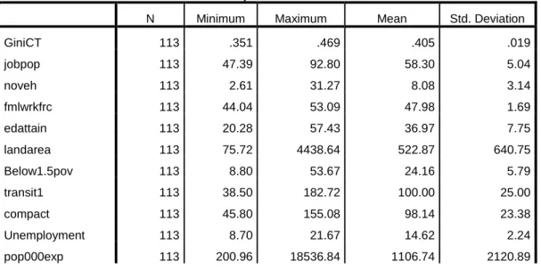
TABLE 2.5 Descriptive Statistics of Final Model Variables
Descriptive Statistics
N Minimum Maximum Mean Std. Deviation
GiniCT 113 .351 .469 .405 .019 jobpop 113 47.39 92.80 58.30 5.04 noveh 113 2.61 31.27 8.08 3.14 fmlwrkfrc 113 44.04 53.09 47.98 1.69 edattain 113 20.28 57.43 36.97 7.75 landarea 113 75.72 4438.64 522.87 640.75 Below1.5pov 113 8.80 53.67 24.16 5.79 transit1 113 38.50 182.72 100.00 25.00 compact 113 45.80 155.08 98.14 23.38 Unemployment 113 8.70 21.67 14.62 2.24 pop000exp 113 200.96 18536.84 1106.74 2120.89
One might notice that the “compact” variable does not, in fact, have a mean of 100 and a standard deviation of 25. This is due to the fact that some cases were lost between the first creation of the database and the inclusion of additional variables for this study.
STRUCTURAL EQUATION MODELING
This study employs structural equation modeling as the principal tool for evaluating relationships between the variables of interest. Structural equation modeling (SEM) is a statistical methodology for evaluating complex hypotheses involving multiple, interacting variables. SEM is a ‘modelcentered’ methodology that seeks to evaluate theoretically justified models against data. The SEM approach is based on the modern statistical view that theoretically based models, when they can be justified on scientific grounds, provide more useful
interpretations than conventional methods that simply seek to reject the ‘null hypothesis’ of no effect. SEM is a series of statistical methods that allow complex relationships between one or
more independent variables and one or more dependent variables. Expert dissertation committee members will be invited to discuss models as they are being formulated and refined.
RESULTS
We developed two models to analyze the effects of exogenous and endogenous variables on income inequality and poverty.
INCOME INEQUALITY MODEL
The income inequality model in Figure 1 has a chi-square of 10.47, with 17 model degrees of freedom, and a p-value of .883. The low chi-square relative to model degrees of freedom, as well as the high p-value indicate good model fit. Additionally, other goodness of fit measures produce promising results. The root mean square error of approximation (RMSEA) of 0.00 falls below the conventional threshold of .05, indicating good model fit. (24) Finally, the comparative fit index (CFI) of 1.00 achieves that measure’s optimum value. All pertinent
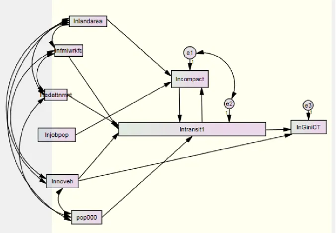
goodness of fit measures indicate this model fits the data well. Below, Figure 2.2 depicts the path diagram produced by the AMOS software.
FIGURE 2.2 Inequality Model SEM Path Diagram
Figure 1 illustrates a path diagram with variables affecting poverty directly and indirectly through endogenous variables. Straight arrows indicate causal pathways, and curved
bidirectional arrows indicate covariances, or correlations. For example, the diagram shows that job-population balance affects compactness, which, in turn, influences transit factor, which directly affects the outcome variable, income inequality. Land area also affects compactness, transit factor, and inequality in the same succession. Female workforce participation, educational attainment, and population directly affect transit factor, which in turn affects inequality. This means that these variables directly affect transit factor, and indirectly affect through through their influence on transit factor.
Model fit, described above, is just part of the process of evaluating models. Next, we compare the relationships described in the model to our theoretical understanding. Table 2.6 includes path coefficient estimates that give the predicted effects of individual variables, ceteris paribus. Estimates can be interpreted as elasticities.
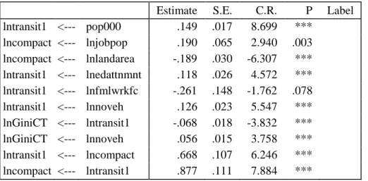
TABLE 2.6 Inequality Model SEM Path Coefficient Estimates
Estimate S.E. C.R. P Label
lntransit1 <--- pop000 .149 .017 8.699 *** lncompact <--- lnjobpop .190 .065 2.940 .003 lncompact <--- lnlandarea -.189 .030 -6.307 *** lntransit1 <--- lnedattnmnt .118 .026 4.572 *** lntransit1 <--- lnfmlwrkfc -.261 .148 -1.762 .078 lntransit1 <--- lnnoveh .126 .023 5.547 *** lnGiniCT <--- lntransit1 -.068 .018 -3.832 *** lnGiniCT <--- lnnoveh .056 .015 3.758 *** lntransit1 <--- lncompact .668 .107 6.246 *** lncompact <--- lntransit1 .877 .111 7.884 ***
All of the path coefficient estimates in Table 2.6 are significant at the standard threshold P < 0.05, except for female workforce proportion, which is significant at the P <0.10 level.
Table 1 specifies that population is positively related to transit and is statistically
significant. Job-population balance positively affects compactness and is statistically significant. Land area negatively affects compactness and is also significant. Educational attainment, no vehicle, and compactness all are positively related to transit factor and their effects are
statistically significant. Female workforce proportion is negatively related to tranit factor and is significant at the P < 0.1 level. Finally, and most importantly, we see that transit factor
negatively affects income inequality. The coefficient of -0.068 means that with an increase in transit factor we can expect to see a small decrease in regional income inequality. This comports with the hypothesis of this paper that transit can act as a moderating factor on spatial mismatch.
Additionally, the small elasticity is expected, given that the majority of cases in the study sample are mid-sized cities in which transit is only a small component of the transportation system, therefore contributing marginally to the regional economy.
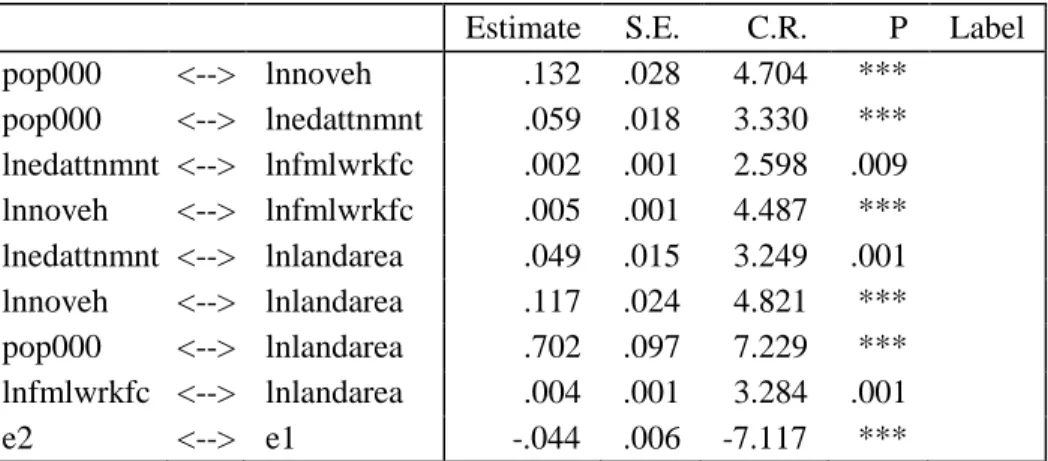
TABLE 2.7 Inequality Model Covariance Estimates
Estimate S.E. C.R. P Label
pop000 <--> lnnoveh .132 .028 4.704 *** pop000 <--> lnedattnmnt .059 .018 3.330 *** lnedattnmnt <--> lnfmlwrkfc .002 .001 2.598 .009 lnnoveh <--> lnfmlwrkfc .005 .001 4.487 *** lnedattnmnt <--> lnlandarea .049 .015 3.249 .001 lnnoveh <--> lnlandarea .117 .024 4.821 *** pop000 <--> lnlandarea .702 .097 7.229 *** lnfmlwrkfc <--> lnlandarea .004 .001 3.284 .001 e2 <--> e1 -.044 .006 -7.117 ***
All the covariances above indicate statistically significant relationships that all agree with our theoretical expectations of the interactions of these variables.
TABLE 2.8 Inequality Model Direct, Indirect, and Total Effects
Direct Effects lnlan darea lnfmlwr kfc lnjobp op lnedattn mnt lnnov eh pop0 00 lncomp act lntransi t1 lncompact -.189 .000 .190 .000 .000 .343 .000 .877 lntransit1 .000 -.261 .000 .118 .126 .149 .668 .000 lnGiniCT .000 .000 .000 .000 .056 .000 .000 -.068
Indirect Effects lnlan darea lnfmlwr kfc lnjobp op lnedattn mnt lnnov eh pop0 00 lncomp act lntransi t1 lncompact -.268 -.553 .270 .250 .266 .315 1.417 1.242 lntransit1 -.305 -.370 .308 .167 .178 .211 .947 1.417 lnGiniCT .021 .043 -.021 -.019 -.021 -.024 -.110 -.096 Total Effects lnlan darea lnfmlwr kfc lnjobp op lnedattn mnt lnnov eh pop0 00 lncomp act lntransi t1 lncompact -.457 -.553 .460 .250 .266 .315 1.417 2.119 lntransit1 -.305 -.631 .308 .285 .304 .359 1.615 1.417 lnGiniCT .021 .043 -.021 -.019 .035 -.024 -.110 -.164
The direct effects depicted above are the same as what we reported in Table 2.7 path coefficient estimates, however, here we also see indirect and total effects of exogenous and endogenous variables on the outcome variable. We see that land area has a positive indirect effect on income inequality through its effect on transit factor. This means that an urbanized area with a larger land area, and thus a higher potential for spatial mismatch, will lead to greater levels of income inequality. This is what we would expect to see, given the theory of spatial mismatch. We see that female workforce participation, job-population balance, educational attainment, no vehicle households, population, and compactness all have negative indirect effects on income inequality through their effects on transit factor. Again, these relationships agree with our theoretical understanding.
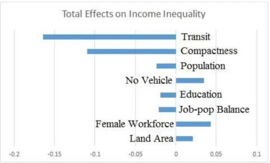
Figure 2.3 graphically depicts total effects of all variables on income inequality.
Figure 2.3 Total Effects on Income Inequality
Figure 2.3 demonstrates that transit has the greatest total effect on income inequality, followed by compactness. The other variables in the model have significantly smaller effects on the outcome variable.
UEMPLOYMENT AND POVERTY MODEL
The poverty model in Figure 3 has a chi-square of 12.97, with 20 model degrees of freedom, and a p-value of .879. The RMSEA of .000 and CFI of 1 also suggest good model fit. Below, Figure 2.4 depicts the path diagram for the poverty model.
FIGURE 2.4 Unemployment and Poverty Model SEM Path Diagram
The path diagram shows some of the same relationships as the inequality model, but is more complex. Here, we have modeled two outcome variables: unemployment and poverty. Another obvious distinction between this and the inequality model is that compactness is directly affecting the outcome variable instead of transit. Here, transit affects unemployment and poverty indirectly through its effect on compactness. Both compactness and transit affect poverty
indirectly through compactness’ effect on unemployment. Another significant difference between this model and the inequality model is that some exogenous variables are directly affecting the outcome variable. This is to be expected, as socioeconomic variables should be directly related to unemployment
TABLE 2.9 Poverty Model SEM Path Coefficient Estimates
Regression Weights:
Estimate S.E. C.R. P Label lntransit1 <--- pop000 .149 .017 8.697 *** lncompact <--- lnjobpop .190 .065 2.941 .003 lncompact <--- lnlandarea -.189 .030 -6.315 *** lntransit1 <--- lnedattnmnt .118 .026 4.571 *** lntransit1 <--- lnfmlwrkfc -.261 .147 -1.772 .076 lntransit1 <--- lnnoveh .126 .023 5.552 *** lnunemployment <--- lncompact -.103 .034 -2.997 .003 lnunemployment <--- lnjobpop -.385 .092 -4.183 *** lnunemployment <--- lnedattnmnt -.397 .048 -8.327 *** lnunemployment <--- lnnoveh .077 .023 3.356 *** lnpoverty <--- lnunemployment 1.838 .249 7.378 *** lntransit1 <--- lncompact .668 .107 6.261 *** lncompact <--- lntransit1 .877 .111 7.904 ***
All the path coefficient estimates in Table 2.9 are significant at the standard threshold of P < 0.05, except for female workforce proportion, which is significant at the P < 0.10 level. This variable persisted to the final model as it performed the best of a group of similar
socioeconomic variables that were tested including race, age, household head, and housing tenure. Table 4 specifies that transit compactness negatively affects unemployment. The
coefficient of -0.103 means that with an increase in compactness we can expect to see a decrease in regional unemployment. In addition, unemployment is positively related to poverty, with a very large elasticity of 1.838. This means that with a positive change in unemployment, we can expect to see an even larger positive change in poverty. In line with the findings of the inequality model, the unemployment and poverty model comports with the hypothesis that transit can act as a moderating factor on spatial mismatch. Although not affecting these outcomes directly, transit contributes to unemployment and poverty indirectly through its effect on compactness.
TABLE 2.10 Unemployment and Poverty Model Covariance Estimates
Estimate S.E. C.R. P Label pop000 <--> lnnoveh .132 .028 4.775 *** pop000 <--> lnedattnmnt .060 .018 3.387 *** lnedattnmnt <--> lnfmlwrkfc .002 .001 2.536 .011 lnnoveh <--> lnfmlwrkfc .005 .001 4.439 *** lnedattnmnt <--> lnlandarea .050 .015 3.302 *** lnnoveh <--> lnlandarea .116 .024 4.896 *** pop000 <--> lnlandarea .701 .096 7.335 *** lnfmlwrkfc <--> lnlandarea .004 .001 3.350 *** e2 <--> e1 -.044 .006 -7.117 *** e4 <--> e3 -.023 .005 -4.793 *** e4 <--> pop000 -.044 .013 -3.513 *** e4 <--> lnlandarea -.039 .012 -3.242 .001
All of the covariances above indicate statistically significant relationships that all agree with our theoretical expectations of the interactions of these variables. It is also heartening that the relationships observed in the poverty model are all quite similar to those observed in the inequality model.
TABLE 2.11 Poverty Model Direct, Indirect, and Total Effects
Direct Effects lnlandare a lnfmlwrkf c lnjobpo p lnedattnm nt lnnove h pop00 0 lncompa ct lntransit 1 lnunemployme nt lncompact -.189 .000 .190 .000 .000 .000 .000 .877 .000 lntransit1 .000 -.261 .000 .118 .126 .149 .668 .000 .000 lnunemployme nt .000 .000 -.385 -.397 .077 .000 -.103 .000 .000 lnpoverty .000 .000 .000 .000 .000 .000 .000 .000 1.838 Indirect Effects lnlandare a lnfmlwrkf c lnjobpo p lnedattnm nt lnnove h pop00 0 lncompa ct lntransit 1 lnunemployme nt lncompact -.268 -.553 .270 .250 .266 .315 1.417 1.242 .000 lntransit1 -.305 -.370 .308 .167 .178 .211 .947 1.417 .000 lnunemployme nt .047 .057 -.047 -.026 -.027 -.032 -.146 -.219 .000 lnpoverty .087 .105 -.795 -.777 .092 -.060 -.458 -.402 .000
Total Effects lnlandare a lnfmlwrkf c lnjobpo p lnedattnm nt lnnove h pop00 0 lncompa ct lntransit 1 lnunemployme nt lncompact -.457 -.553 .460 .250 .266 .315 1.417 2.119 .000 lntransit1 -.305 -.631 .308 .285 .304 .359 1.615 1.417 .000 lnunemployme nt .047 .057 -.432 -.422 .050 -.032 -.249 -.219 .000 lnpoverty .087 .105 -.795 -.777 .092 -.060 -.458 -.402 1.838
We see that land area has a positive total effect on unemployment and poverty, mediated through its effects on transit and compactness. Similarly, female workforce proportion
contributes to an increase in unemployment and poverty through its relationship with transit and compactness. The remaining relationships can be interpreted in the same manner. Below, Figures 2.5 and 2.6 depict the total effects of the explanatory variables on the outcome variables.
Figure 2.5 highlights that compactness has a slightly larger total effect on unemployment than poverty, both with elasticities just slightly larger than -0.2. However, we should note that education and job-population balance demonstrate much larger elasticities than those of transit and compactness. With an outcome variable of unemployment, it would follow that education is highly impactful on unemployment. However, the finding that job-population balance is very influential on unemployment is remarkable. While many have shown that an ideal job-population balance can lead to different transportation outcomes as well as income matching (Cervero, 1989; Zhao, Lu, & Roo, 2011; Stoker & Ewing, 2014), the connection between this variable and regional unemployment has yet to be made. We find that job-population balance is a strong determinant of regional unemployment, with an elasticity of -0.432.
FIGURE 2.6 Total Effects on Poverty
The total effects of the explanatory variables on poverty are similar in their effects relative to each other; however, the effects are magnified as compared to what we observe with
unemployment. This magnification of total effects is due to the highly elastic relationship between unemployment and poverty.
CONCLUSION
The results of this study support the theory that transit can act as a moderator on the relationship between spatial mismatch and unemployment and poverty. Our models indicate that transit, measured as a factor of many indicators of transit service provision, has a negative indirect effect on unemployment and poverty through its effect on compactness. Relatively large elasticities of transit on unemployment and poverty suggest that supporting transit service can act as an effective lever on regional economies. Our models also demonstrate that transit can directly affect income inequality, although to a lesser degree than its total effects on unemployment and poverty. Again, these findings are similar to what we would expect, and support the theory that transit moderates the problem of spatial mismatch. Finally, we find that jobs-housing balance is highly influential on regional unemployment and poverty, even more so than transit and
compactness.
The finding that transit limits regional unemployment and poverty is the most significant contribution of this study. The fact that a robust transit system can affect regional economic outcomes is notable because it offers a new possible lever for policy makers. Policies aimed at lifting economies and limiting the effects of economic hardship are numerous, wide-ranging, and often esoteric. However, this study give credence to the long-held but mostly unproven theory that transportation spending, specifically spending on transit systems, can help to boost regional economies. The empirical connection established in this paper between transit service and
regional economies strengthens the case for policy makers to support spending on transit with the purpose of improving economic opportunities can use reductions in unemployment and poverty.
When we model transit’s effect on unemployment directly, we see models with poorer fit, and a non-significant relationship between transit and unemployment. This indicates that it is unlikely that transit affects unemployment directly, or if it does, its effects are not measureable at the regional level. In a conversation with an academic leader in transit and equity, he suggested that our models would not be able to detect a relationship between transit and unemployment because the majority of transit systems in the US are too small to be able to observe common variation between transit and economic outcomes. The lack of a direct effect of transit on unemployment vindicates this assertion, but only to some degree. We find that even if the direct variation between the two variables is too small to detect or non-existent, an indirect effect of transit on unemployment is, in fact, measurable and noteworthy.
Another important result of our models is the discovery that while transit affects unemployment and poverty only indirectly through compactness, it affects income inequality directly. Similar to what we describe above, when we model the effect of transit on income inequality indirectly through compactness, as it is done in the unemployment and poverty model, we observe poorer model fit and an insignificant relationship with the incorrect sign. However, when the relationship of transit on income inequality is modeled directly, the model fit improves. The direct effect of transit on income inequality is small, with an elasticity of only -0.07,
however, when the indirect effect is included, the total effect is -0.16. This is still a relatively small elasticity, but it is not trivial. Transit’s elasticity of -0.16 with respect to income inequality indicates that as transit service increases, we can expect to see a small reduction in regional income inequality.
This paper also suggests that land use planning can have an effect on regional economic outcomes. Job-population balance has been associated with transportation behavior and income matching in the past, but it has yet to be tied to unemployment and poverty. We find that job-population balance is highly influential on these outcomes. This advances the notion that successful land use planning in which a proper balance of jobs and population is achieved can have an impact on unemployment and poverty. This suggests that planners can have lasting effects on economic development. Additionally, we also see further evidence for the theory of spatial mismatch. A proper balance of jobs and population would create more opportunities for jobs to be located near the residences of workers, and the results of our models support this theory.
LIMITATIONS
This paper represents a major step forward in empirically understanding the theory of transit service’s effects on spatial mismatch. Using data from a national sample of the largest US cities helps us to understand how quality transit relates to regional economic outcomes.
However, we must briefly discuss how the study design limits how we can interpret the results. The cross-sectional nature of the dataset offers a degree of generalizability of the results, but it also limits our ability to attribute causality to the relationships we modeled. An assumption of inferential association in cross-sectional study design is that the difference observed between observations is random. This means that the difference in attributes associated with a specific location are related to the that locations attributes alone, and not associated with its location itself. Geography is inextricably linked to urban phenomenon, and as such, there are limitations to cross-sectional study designs in this field.
An additional limitation to our study is the inherent issue of ecological fallacy associated with explaining phenomena that are experienced at the individual or household level but
measured at an aggregated level. We can say that regions with higher quality transit and more compactness are likely to experience lower unemployment and poverty rates, but not that a certain level of transit provision will provide the requisite level of economic opportunity for a specific household or individual. Finally, there is the unavoidable issue of endogeneity associated with modeling complex relationships using interrelated variables. We have
constructed our models in a way that is theoretically justifiable, but one could certainly make arguments against whether any of the variables said to be exogenous in our models are, in fact so. Structural equation modeling requires the organization of variables in this fashion, and we also believe that our models represent relationships that are structured in a logical and
REFERENCES
Achia, T., Wangombe, A., and Khadioli N. (2010). A Logistic Regression Model to Identify Key Determinants of Poverty Using Demographic and Health Survey Data, European Journal of Social Sciences,13 (1) 38-45
Badinger, H., & Url, T. (2002). Determinants of regional unemployment: some evidence from Austria. Regional studies, 36(9), 977-988.
Bakija, J., Cole, A., & Heim, B. T. (2012). Jobs and income growth of top earners and the causes
of changing income inequality: Evidence from US tax return data. Unpublished
manuscript, Williams College.
Berechman, J., Ozmen, D., & Ozbay, K. (2006). Empirical analysis of transportation investment
and economic development at state, county and municipality levels. Transportation,
33(6), 537-551.
Blanden, J. (2013). Cross‐country rankings in intergenerational mobility: a comparison of
approaches from economics and sociology. Journal of Economic Surveys, 27(1), 38-73.
Bratberg, E., Davis, J., Mazumder, B., Nybom, M., Schnitzlein, D. D., & Vaage, K. (2017). A Comparison of Intergenerational Mobility Curves in Germany, Norway, Sweden, and the US. The Scandinavian Journal of Economics, 119(1), 72-101.
Cervero, R., & Duncan, M. (2006). 'Which Reduces Vehicle Travel More: Jobs-Housing Balance
or Retail-Housing Mixing?. Journal of the American planning association, 72(4), 475-
490.
Cervero, R. (1989). Jobs-housing balancing and regional mobility. Journal of the American
Planning Association, 55(2), 136-150.
Cervero, R., Sandoval, O., & Landis, J. (2002). Transportation as a stimulus of welfare-to-work:
Private versus public mobility. Journal of Planning Education and Research, 22(1),
50-63.
Chetty, R., Hendren, N., Kline, P., & Saez, E. (2014). Where is the land of opportunity? The
geography of intergenerational mobility in the United States. The Quarterly Journal of
Economics, 129(4), 1553-1623.
The Journal of Economic Perspectives, 27(3), 79-102.
Cingano, F. (2014). Trends in income inequality and its impact on economic growth.
Dabla-Norris, M. E., Kochhar, M. K., Suphaphiphat, M. N., Ricka, M. F., & Tsounta, E. (2015).
Causes and consequences of income inequality: a global perspective. International Monetary Fund.
Ellwood, D. T. (1986). The spatial mismatch hypothesis: Are there teen-age jobs missing in the ghetto? In R. B. Freeman & H. J. Holzer (Eds.), The black youth employment crisis (pp. 147– 190). Chicago: University of Chicago Press.
Ewing, R., Hamidi, S., Grace, J. B., & Wei, Y. D. (2016). Does urban sprawl hold down upward
mobility?. Landscape and Urban Planning, 148, 80-88.
Ewing, R., Meakins, G., Hamidi, S., & Nelson, A. C. (2014). Relationship between urban sprawl
and physical activity, obesity, and morbidity–update and refinement. Health & place, 26,
118-126.
Ewing, R., Hamidi, S., Tian, G., Proffitt, D., Tonin, S., & Fregolent, L. (2018). Testing Newman
and Kenworthy’s theory of density and automobile dependence. Journal of Planning
Education and Research, 38(2), 167-182.
Filiztekin, A. (2009). Regional unemployment in Turkey. Papers in regional science, 88(4), 863- 878.
Förster, M. F., & Pellizzari, M. (2000). Trends and driving factors in income distribution and poverty in the OECD area.
Harper, C., Marcus, R., & Moore, K. (2003). Enduring poverty and the conditions of childhood:
lifecourse and intergenerational poverty transmissions. World development, 31(3),
535-554.
Horrell, S., Humphries, J., & Voth, H. J. (2001). Destined for deprivation: Human capital
formation and intergenerational poverty in nineteenth-century England. Explorations in
Economic History, 38(3), 339-365.
Ihlanfeldt, K. R. (1993). Intra-urban job accessibility and Hispanic youth employment
rates. Journal of Urban Economics, 33(2), 254-271.
Kain, J. H., & Persky, J. J. (1969). Alternatives to the gilded ghetto. The Public Interest, (14), 74.
Kaplan, G. A., Pamuk, E. R., Lynch, J. W., Cohen, R. D., & Balfour, J. L. (1996). Inequality in income and mortality in the United States: analysis of mortality and potential pathways.
Bmj, 312(7037), 999-1003.
Kasarda, J. D. (1983). Entry-level jobs, mobility, and urban minority unemployment. Urban
Affairs Quarterly, 19(1), 21-40.
Kuznets, S. (1955). Economic growth and income inequality. The American economic review,
1-28.
Landersø, R., & Heckman, J. J. (2017). The scandinavian fantasy: The sources of
intergenerational mobility in denmark and the us. The Scandinavian Journal of
Economics, 119(1), 178-230.
Moller, S., Huber, E., Stephens, J. D., Bradley, D., & Nielsen, F. (2003). Determinants of relative poverty in advanced capitalist democracies. American sociological review, 22- 51.
Moore, K. (2005). Thinking about youth poverty through the lenses of chronic poverty, life-course poverty and intergenerational poverty.
Piachaud, D. (2002). Capital and the determinants of poverty and social exclusion.
Reed, D. (1999). California's rising income inequality: Causes and concerns. San Francisco:
Public Policy Institute of California.
Rupasingha, A., & Goetz, S. J. (2007). Social and political forces as determinants of poverty: A spatial analysis. The Journal of Socio-Economics, 36(4), 650-671.
Sanchez, T. W. (1999). The connection between public transit and employment: the cases of
Portland and Atlanta. Journal of the American Planning Association, 65(3), 284-296.
Sanchez, T. W. (2008). Poverty, policy, and public transportation. Transportation Research Part
A: Policy and Practice, 42(5), 833-841.
Stoker, P., & Ewing, R. (2014). Job–worker balance and income match in the United States.
Housing Policy Debate, 24(2), 485-497.
Tian, G., Ewing, R., White, A., Hamidi, S., Walters, J., Goates, J. P., & Joyce, A. (2015). Traffic generated by mixed-use developments: Thirteen-region study using consistent measures
of built environment. Transportation Research Record: Journal of the Transportation
Research Board, (2500), 116-124.
American Planning Association, Planning Advisory Service.
Wolf, J. P. (2007). Sociological theories of poverty in urban America. Journal of Human
Behavior in the Social Environment, 16(1-2), 41-56.
Zenou, Y. (2000). Urban unemployment, agglomeration and transportation policies. Journal of
Public Economics, 77(1), 97-133.
Zhao, P., Lü, B., & De Roo, G. (2011). Impact of the jobs-housing balance on urban commuting
CHAPTER 3:
TRANSIT ECONOMIC EQUITY
INDEX: DEVELOPING A
COMPREHENSIVE MEASURE OF
TRANSIT SERVICE EQUITY
ABSTRACT:
In this study we develop an index that we call the Transit Economic Equity Index to quantitatively assess transit service equity. The index measures convenience of travel for
advantaged and disadvantaged work trips based on travel speed using a multimodal network that includes transit lines, stop locations, transit schedules, and pedestrian connections via the street network. Non-peak hour service is compared with peak-hour service to determine the degree to which operating resources are concentrated in times that might have greater benefits to
advantaged populations. Finally, we compare accessibility to the transit system in terms of the number of transit stops in neighborhoods and employment centers and compare these figures between advantaged and disadvantaged locations. The scores for these three components are combined to create a single measure of transit economic equity. We define disadvantage using criteria established in Title VI of the Civil Rights Act of 1964. We have constructed the index in a way that balances a robust and meaningful measure of transit equity with the ability to be replicated relatively easily so that transit agencies can reasonably use this metric to assess the equity of their systems as well as how potential service changes affect equity.
INTRODUCTION:
Transit agencies and other public institutions use performance measures to assess their ability to successfully provide services and achieve their goals and objectives. The most common performance measurement of transit agencies is transit ridership. This measure is of the utmost importance to transit agencies as it is an effective proxy for the ability of a transit system to provide mobility and access to opportunities for travelers not using private vehicles. However, with the supremacy of this measure comes the potential to make decisions that are favorable in terms of their effects on ridership, but possibly not beneficial in terms of equity. While equity and ridership are not necessarily competing goals, measuring just one of these performance measures demonstrates a priority that may not accurately reflect the goals and objectives of a transit agency. Measuring equity as well as ridership will help transit agencies to make better decisions that find a balance of these two goals.
Transit agencies are required to analyze the effects of service changes on equity through Title VI of the Civil Rights Act of 1964. Changes in service that are found to have a disparate impact on disadvantaged populations, defined by race and income, are determined to be inequitable. This analysis is required of agencies serving populations greater than 200,000 receiving federal transportation funds. The spirit of the regulation is to ensure that federal transportation spending is not being unfairly allocated to already advantaged groups.