Workshop on Data Mining for Computer Security

Workshop on

Data Mining for Computer Security

www.cs.fit.edu/~pkc/dmsec03/

in conjunction with

IEEE International Conference on Data Mining

November 19-22, 2003

Melbourne, Florida

Workshop Organizers:

Philip Chan, Florida Tech

Vipin Kumar, University of Minnesota

Wenke Lee, Georgia Tech

Program Committee:

•

Wenke Lee, Georgia Tech (Co-Chair)

•

Srinivasan Parthasarathy, Ohio State U (Co-Chair)

•

Daniel Barbara, GMU

•

Philip Chan, Florida Tech

•

Eleazar Eskin, Hebrew U

•

Wei Fan, IBM Watson

•

Anup Ghosh, DARPA

•

Sushil Jajodia, GMU

•

Vipin Kumar, U. Minnesota

•

Terran Lane, U. New Mexico

•

Aleksandar Lazarevic, U. Minnesota

•

Richard Lippmann, MIT Lincoln Lab

•

Matthew Mahoney, Florida Tech

•

Roy Maxion, CMU

•

Chris Michael, Cigital

•

R. Sekar, Stony Brook U

•

Jaideep Srivastava, U. Minnesota

•

Salvatore Stolfo, Columbia U

•

Kymie Tan, CMU

•

Alfonso Valdes, SRI

External Reviewers:

•

Zoran Duric, George Mason University

•

Eric Eilertson, University of Minnesota

•

Levent Ertoz, University of Minnesota

•

Amol Ghoting, Ohio State University

•

Matthew Otey, Ohio State University

•

Aysel Ozgur, University of Minnesota

•

Joseph Pamula, George Mason University

•

Xinzhou Qin, Georgia Institute of Technology

•

Sankardas Roy, George Mason University

TABLE OF CONTENTS

INVITED TALKS

Authenticating Users by Profiling Behavior 1

Tom Goldring, NSA

Behavior-based Security 1

Salvatore J. Stolfo, Columbia University

ANOMALY DETECTION

One Class Support Vector Machines for Detecting Anomalous Windows 2

Registry Accesses

Katherine Heller, Krysta Svore, Angelos Keromytis, and Salvatore Stolfo [Columbia University]

One Class Training for Masquerade Detection 10

Ke Wang and Salvatore J. Stolfo [Columbia University]

Learning Rules from System Call Arguments and Sequences for Anomaly 20

Detection

Gaurav Tandon and Philip Chan [Florida Institute of Technology]

Detection of Novel Network Attacks Using Data Mining 30

Levent Ertoz, Eric Eilertson , Aleksandar Lazarevic, Pang-Ning Tan, Paul Dokas, Vipin Kumar, and Jaideep Srivastava [University of Minnesota]

FEATURE EXTRACTION

Passive Operating System Identification from TCP/IP Packet Headers 40 Richard Lippmann, David Fried, Keith Piwowarski, and William Streilein

[MIT Lincoln Laboratory]

Boundary Detection in Tokenizing Network Application Payload for 50

Anomaly Detection

Rachna Vargiya and Philip Chan [Florida Institute of Technology]

MISUSE DETECTION

Detecting Privilege-Escalating Executable Exploits 60

Jesse C. Rabek, Robert K. Cunningham, and Roger I. Khazan [MIT Lincoln Laboratory]

VISUALIZATION

A Prototype Tool for Visual Data Mining of Network Traffic for Intrusion Detection 67 William Yurcik, Kiran Lakkaraju, James Barlow and Jeff Rosendale

Introduction

Computer security is a broad field that encompasses issues both theoretical and practical aspects. It

is of incredible importance to a wide variety of practical domains ranging from the banking

industry to multi-national corporations, from space exploration to the intelligence community and

so on. Computer security is frequently associated with three core areas: confidentiality, integrity

and authentication. Although security policies and mechanisms address all three of these areas,

they are not perfect and more and more organizations are becoming vulnerable to a wide variety of

security breaches due to decreasing cost of the information processing and Internet accessibility.

The most common security breaches include different cyber attacks to single computers, computer

networks, wireless networks, databases or authentication compromises (e.g. masquerading).

The main aim of this workshop is to bring together leading figures from academia, government and

industry to explore the applications of data mining in computer security.

Presentations in this workshop focus on several aspects of computer security, mainly in the area of

intrusion detection. They are organized in the following four sessions:

•

Anomaly Detection

•

Feature Extraction

•

Misuse Detection

•

Visualization

The first session presents different data mining based anomaly detection techniques for recognizing

novel and emerging computer attacks. Papers in the feature extraction session investigate various

attributes that may be beneficial in data mining based techniques for intrusion detection. The paper

in the misuse detection session presents a statistical based detector of malicious codes, while in the

visualization session new data mining based prototype is presented to help security analysts to

interactively assess security situational awareness of an entire network traffic.

The workshop program contains 8 papers selected from 17 submissions after a peer review process.

Since two of the organizers (Chan and Kumar) submitted papers to the workshop, the other two

organizers (Lee and Parthasarathy) organized the reviewing process and made the decisions on

paper acceptance to avoid conflicts of interests. Three reviews were sought for each paper -- in

select cases a fourth review was solicited either in the event of a missing review or in the event of

low-confidence reviews. We like to thank the program committee members and external reviewers

for their help in reviewing the submissions and providing comments for the authors. Special thanks

are due to Xinzhou Qin (Georgia Tech) for setting up the workshop management system that

facilitated paper submission and reviewing, and to Aleksandar Lazarevic (University of Minnesota)

for workshop publicity as well as putting together the workshop proceedings. Lastly, we would like

to express our appreciation to Tom Goldring for his invited talk on “Authenticating Users by

Profiling Behavior” and Sal Stolfo on “Behavior-based Security”.

INVITED TALKS

Authenticating Users by Profiling Behavior

Tom

Goldring,

NSA

Building profiles of computer user activity entails collecting user session data, then learning models from this data, which can be used to classify new sessions. From the Computer Security viewpoint, the purpose would be to authenticate logins and detect insider misuse. A good data source will reflect user behavior and allow us to filter out system noise, both with a high degree of accuracy. Numerous published studies have used command line data, but this is probably no longer a viable source in today's environment.

The next step is feature selection, which allows us to choose among various existing classification algorithms to solve the authentication problem. But even the best algorithms will perform badly if the features are poor. Depending on what the data looks like, finding the right features and coaxing them into a usable form can be nontrivial. For nearly two years we have been monitoring "real" users on an operational Windows NT network that was part of a closed, internal network laboratory. In this talk we will describe our data, discuss the features we are currently using, and present results obtained to date.

Behavior-based Security

Salvatore J. Stolfo, Columbia University

Abstract. Behavior-based security systems are a new generation of computer security technologies that defend and protect critical IT assets by detecting deviations from a system's normal behavior. Behavior-based security systems provide the means of detecting attacks from remote sources, and from within, i.e. the insider problem.

The Email Mining Toolkit (EMT) is a data mining system that computes behavior profiles or models of user email accounts. These models may be used for a variety of forensic analyses and detection tasks. In this talk we describe the application of these models to detect the early onset of a viral propagation without "content-based" (or signature-based) analysis in common use in virus scanners. We present several experiments using real email from 15 users with injected simulated viral emails and describe how the combination of different behavior models improves overall detection rates. The performance results vary depending upon parameter settings, approaching 99% true positive (TP) (percentage of viral emails caught) in general cases and with 0.38% false positive (FP) (percentage of emails with attachments that are mislabeled as viral).

The principle behind behavior-based security is to model communication flows between systems and users, (possibly including content) using well grounded statistical techniques. The statistics gathered may be used to determine "social clique and communication communities" that typically exchange information, and the frequency of messages and the typical times and days those messages are exchanged. All this information can be used to model accounts, hosts or systems to determine typical behaviors that may be used to detect deviations of interest that may indicate misbehavior or security breaches.

We believe EMT thus serves as a model anomaly detection system for any audit stream and detection problem of interest. This work suggests a general framework that is the subject matter of our ongoing work. This framework posits that anomaly detection is best cast as a problem to optimally correlate multiple detectors, where each detector models normal behavior using different features of the audit stream. These detectors generate alerts when there are violations of volume and velocity statistics, anomalous values exhibited in an audit stream, and abnormal or inconsistent formation of vertices when viewing data in the audit stream in graph theoretic formulations. All of these concepts and modeling techniques are embodied in EMT.

One Class Support Vector Machines for Detecting Anomalous Windows Registry

Accesses

Katherine A. Heller

Krysta M. Svore

Angelos D. Keromytis

Salvatore J. Stolfo

Dept. of Computer Science

Columbia University

1214 Amsterdam Avenue

New York, NY 10025

heller,kmsvore,angelos,sal

@cs.columbia.edu

Abstract

We present a new Host-based Intrusion Detection Sys-tem (IDS) that monitors accesses to the Microsoft Windows Registry using Registry Anomaly Detection (RAD). Our sys-tem uses a one class Support Vector Machine (OCSVM) to detect anomalous registry behavior by training on a dataset of normal registry accesses. It then uses this model to de-tect outliers in new (unclassified) data generated from the same system. Given the success of OCSVMs in other ap-plications, we apply them to the Windows Registry anomaly detection problem. We compare our system to the RAD sys-tem using the Probabilistic Anomaly Detection (PAD) algo-rithm on the same dataset. Surprisingly, we find that PAD outperforms our OCSVM system due to properties of the hi-erarchical prior incorporated in the PAD algorithm. In the future, these properties may be used to develop an improved kernel and increase the performance of the OCSVM system.

1. Introduction

One of the most popular and most often attacked oper-ating systems is Microsoft Windows. Malicious software is often run on the host machine to inflict attacks on the system. Several methods can be used to combat malicious attacks, such as virus scanners and security patches. How-ever, these methods are not able to combat unknown at-tacks, so frequent updates of the virus signatures and se-curity patches must be made.

An alternative to these methods is a Host-based Intru-sion Detection System (IDS). Host-based IDS systems de-tect intrusions on a host system by monitoring system ac-cesses. Most IDS systems utilize signature based algo-rithms that rely on knowing the attacks and their signatures,

which limits their ability to detect unknown attack meth-ods. Alternatively, “behavior-blocking” technology aims to detect and stop malicious activities using a set of signature-based descriptions of good behavior, i.e. what is expected of program or system execution. To improve performance, data mining techniques have recently been applied to IDS systems [20, 22] to automatically learn models of “good behavior” and “bad behavior” by observing a system un-der normal operation. In this paper, we describe a new approach based on anomaly detection, utilizing a method that trains on normal data and looks for anomalous behav-ior that deviates from the normal model [11, 12, 13]. This method can better identify unknown attacks. Previous work using IDS systems has been done using system call anal-ysis [14, 15, 17, 19, 24] and network intrusion detection [13, 18, 21].

We use the Registry Anomaly Detection (RAD) system to monitor Windows registry queries [9]. During normal computer activity, a certain set of registry keys are typi-cally accessed by Windows programs. Users tend to use certain programs regularly, so registry activity is fairly reg-ular and thus provides a good platform to detect anomalous behavior. We apply an OCSVM algorithm to the RAD sys-tem to detect anomalous activity in the windows registry. Although OCSVMs have previously been applied success-fully to other anomaly detection problems, they have never before been used to detect anomalous accesses to the Win-dows registry. The OCSVM builds a model from training on normal data and then classifies test data as either normal or attack based on its geometrical deviation from the nor-mal training data [23]. We present our results of the RAD system using the OCSVM algorithm and demonstrate its abilities to detect anomalous behavior with several different kernels. We also compare our system with work done on the RAD system using the Probabilistic Anomaly Detection (PAD) algorithm [14, 9]. PAD outperforms the OCSVM

system due to the use of the estimator developed by Fried-man and Singer [16]. This estimator uses a Dirichlet-based hierarchical prior to smooth the distribution and account for the likelihoods of unobserved elements in sparse data sets by adjusting their probability mass based on the number of values seen during training. An understanding of the ferences between these two models and the reasons for dif-ferences in detection performance may help to construct a more discriminative kernel, and is critical to the develop-ment of effective anomaly detection systems in the future.

2. The Windows Registry and the RAD system

The Windows registry is a database that stores config-uration settings for programs, security information, user profiles, and many other system parameters. The registry consists of entries, which are called registry keys, and their associated values. Programs query the registry for infor-mation by accessing a specific registry key. Each registry query has five components: the name of the process, the type of query, an associated key, the result, and the success status of the query. The process may be an attack or normal process. Each record in both our test dataset and training dataset contains all five of these entries. A sample record entry appears as:

Process:EXPLORER.EXE Query:OpenKey Key:HKCR\CLSID\B41DB860-8EE4-11D2-9906 -E49FADC173CA\shellex\MayChange DefaultMenu Response:SUCCESS ResultValue:NOTFOUND

The Registry Anomaly Detection (RAD) system has three parts: an audit sensor, a model generator, and an anomaly detector. Each registry access is either stored as a record in the training set or sent to the detector for anal-ysis by the audit sensor. The model generator develops a model of normal behavior from the training dataset, and the anomaly detector uses this model to classify new registry accesses as normal or anomalous.

The Registry Anomaly Detection (RAD) system utilizes the five raw features given above, such that the algorithm used for anomaly detection classifies each entry as either normal or attack according to these feature values. The pro-cess is the name of the propro-cess querying the registry. The query is the type of access being sent to the registry. The key is the key currently being accessed. The response is the outcome of the query. The value of the accessed key is the result value. For more detailed information on RAD and the Windows registry, refer to [9].

3. The PAD Algorithm

The Probabilistic Anomaly Detection (PAD) algorithm, developed by Eskin [14, 9], trains a model over normal data features. It is essentially density estimation, where the esti-mation of a density function over normal data allows the definition of anomalies as data elements that occur with low probability. The detection of low probability data (or events) are represented as consistency checks over the nor-mal data, where a record is labeled anonor-malous if it fails any one of these tests.

First and second order consistency checks are applied. First order consistency checks verify that a value is consis-tent with observed values of that feature in the normal data set. It computes the likelihood of an observation of a given feature, , where are the feature variables. Second order consistency checks determine the conditional proba-bility of a feature value given another feature value, denoted by , where and are the feature variables.

One way to compute these probabilities would be to esti-mate a multinomial that computes the ratio of the counts of a given element to the total counts. However, this results in a biased estimator when there is a sparse data set. Instead, the estimator given by Friedman and Singer is used to de-termine these probability distributions [16]. Let be the total number of observations, be the number of obser-vations of symbol, be the “pseudo count” that is added to the count of each observed symbol, be the number of observed symbols, and be the total number of possible symbols. Then the probability for an observed element is given by: (1) and the probability for an unobserved element is:

!"# $ &%' $ % (2)

where , the scaling factor, accounts for the likelihood of observing a previously observed element versus an unob-served element. In [16], they compute as:

()+* ,.-/,.0 1 2 43 , 56) ,87,.0 3 , :9<; (3) where 3 , =?>@AB ,DC ,.-E,.0GFBH ,5IKJ FBH ,5IKLNMOJ and 6>PB is a prior probability associated with the size of the subset of elements in the alphabet that have non-zero probability.

In PAD, however, the above computation of is too costly, so a heuristic method is used, where is given by:

&%'

They normalize the consistency check to account for the number of possible outcomes of by considering if is the probability estimated from the consistency check, then they report?2

$

+? ? .

Since there are five feature values for each record in the RAD system, there are 5 first order consistency checks and 20 second order consistency checks. A record is labeled anomalous if any of the 25 consistency checks is below a given threshold. This method labels every record in the dataset as normal or anomalous. To improve the detection rate, pairs of features are examined since a record may have a set of feature values that are inconsistent even though all single feature values are consistent for that record. Most attacks effect a large number of records.

The PAD algorithm takes time , where is the number of unique record values for each record component and is the number of record components. The space re-quired to run the algorithm is .

4.

One

Class

Support

Vector

Machine

(OCSVM)

Instead of using PAD for model generation and anomaly detection, we apply an algorithm based on the one class SVM algorithm given in [23]. Previously, OCSVMs have not been used in Host-based anomaly detection systems. The OCSVM code was developed by [10] and has been modified to compute kernel entries dynamically due to memory limitations. The OCSVM algorithm maps input data into a high dimensional feature space (via a kernel) and iteratively finds the maximal margin hyperplane which best separates the training data from the origin. The OCSVM may be viewed as a regular two-class SVM where all the training data lies in the first class, and the origin is taken as the only member of the second class. Thus, the hyperplane (or linear decision boundary) corresponds to the classifica-tion rule:

/#

(5)

where is the normal vector and is a bias term. The OCSVM solves an optimization problem to find the rule

with maximal geometric margin. We can use this classifica-tion rule to assign a label to a test example . If

/! we label as an anomaly, otherwise it is labeled normal. In practice there is a trade-off between maximizing the dis-tance of the hyperplane from the origin and the number of training data points contained in the region separated from the origin by the hyperplane.

4.1.

Kernels

Solving the OCSVM optimization problem is equivalent to solving the dual quadratic programming problem:

"$#&% I $ '( E?<) *28 (6)

subject to the constraints

$+ + $ , (7) and ( $ (8)

where is a lagrange multiplier (or “weight” on exam-ple such that vectors associated with non-zero weights are called “support vectors” and solely determine the optimal hyperplane),,

is a parameter that controls the trade-off be-tween maximizing the distance of the hyperplane from the origin and the number of data points contained by the hyper-plane, is the number of points in the training dataset, and ) -2 is the kernel function. By using the kernel func-tion to project input vectors into a feature space, we allow for nonlinear decision boundaries. Given a feature map:

.0/ 2143 M (9) where .

maps training vectors from input space to a high-dimensional feature space, we can define the kernel function as: ) -52#6 . 7 . 5B (10)

Feature vectors need not be computed explicitly, and in fact it greatly improves computational efficiency to directly compute kernel values ) 5B. We used three common kernels in our experiments:

Linear kernel:) 5B# 98:52 Polynomial kernel: ) -52OP;85

$

-< , where= is the degree of the polynomial

Gaussian kernel: ) -5B?> 9A@CB 9EDF@CG-H H JI G J , whereKL is the variance

Our OCSVM algorithm uses sequential minimal opti-mization to solve the quadratic programming problem, and therefore takes time = NM8 , where= is the number of di-mensions and is the number of records in the training dataset. Typically, since we are mapping into a high dimen-sional feature space d exceedsO from the PAD complex-ity. Also for large training setsNM will significantly exceed , thereby causing the OCSVM algorithm to be a much

more computationally expensive algorithm than PAD. An open question remains as to how we can make the OCSVM system in high bandwidth real time environments work well and efficiently. All feature values for every example must be read into memory, so the required space is = ? , where is the number of records in the test dataset. Al-though this is more space efficient than PAD, we compute our kernel values dynamically in order to conserve mem-ory, resulting in the added d term to our time complexity. If we did not do this the memory needed to run this algo-rithm would would be = ? D which is far too large to fit in memory on a standard computer for large training sets (which are inherent to the windows anomaly detection problem).

5. Experiments and Results

The one class SVM system we develop detects abnormal accesses to the Windows registry. The training and testing datasets were developed from real usage of the Windows system, and each experiment took one to two weeks to run on a 1.5GHZ Pentium IV dual processor. The training data we used was collected on Windows NT 4.0 and consists of approximately 500,000 free records. These attack-free records are labeled normal and consist of operating sys-tem programs and typical Windows programs. The test data consists of approximately 300,000 records of which approx-imately 2,000 are labeled attacks. Possible attacks include aimrecover, browslist, setuptrojan, and other publicly avail-able attacks [1, 2, 3, 4, 5, 6, 7, 8].

We obtained kernels from binary feature vectors by map-ping each record into a feature space such that there is one dimension for every unique entry for each of the five given record values. This means that a particular record has the value 1 in the dimensions which correspond to each of its five specific record entries, and the value 0 for every other dimension in feature space. We then computed linear ker-nels, second order polynomial kerker-nels, and gaussian kernels using these feature vectors for each record.

We also computed kernels from frequency-based feature vectors such that for any given record, each feature cor-responds to the number of occurences of the correspond-ing record component in the traincorrespond-ing set. For example, if the second component of a record occurs three times in the training set, the second feature value for that record is three. We then used these frequency-based feature vectors to com-pute linear and polynomial kernels.

To evaluate the system’s accuracy, two statistics have been computed: detection rate and false positive rate. The detection rate is the percentage of attack records that have been correctly identified. The false positive rate is the per-centage of normal records that have been mislabeled as anomalous. The threshold is the value that determines if

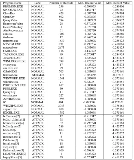
Threshold False Positive Rate (%) Detection Rate (%) -1.08307 0.790142 0.373533 -1.08233 0.828005 0.480256 -1.07139 1.54441 0.533618 -0.968913 1.65734 1.17396 -0.798767 3.58736 3.89541 -0.79858 3.63784 5.60299 -0.798347 3.68999 6.77695 -0.767411 3.72054 6.83031 -0.746663 4.35691 7.47065 -0.746616 4.63025 8.00427 -0.71255 8.34283 20.9712 -0.712503 8.75201 22.0918

Table 1. The effects of varying the threshold on the false positive rate and the detection rate.

a record is normal or attack. Table 1 includes a sample of the varying thresholds and their effects on the detection rate and false positive rate.

0 10 20 30 40 50 60 70 80 90 100 0 10 20 30 40 50 60 70 80 90 100

Percentage of Normal Data Labeled Anomalies

Percentage of True Anomalies Correctly Identified

PAD Binary Gaussian Binary Polynomial (degree 2) Binary Linear

Figure 1. ROC curve for the kernels using bi-nary feature vectors (false positives versus true positives).

We can measure the performance of the one class SVM on our test data by plotting its Receiver Operator Charac-teristic (ROC) curve. The ROC curve plots the percentage of false positives (normal records labeled as attacks) versus the percentage of true positives. As the discriminant thresh-old increases, more records are labeled as attacks. Ran-dom classification results in 50% of the area lying under the curve, while perfect classification results in 100% of the area lying under the curve. Results from our one class SVM system are shown with the results of the PAD system on the same dataset in Figures 1 and 2. Figure 1 is the ROC curve for the linear and polynomial kernels using binary feature

0 10 20 30 40 50 60 70 80 90 100 0 10 20 30 40 50 60 70 80 90 100

Percentage of Normal Data Labeled Anomalies

Percentage of True Anomalies Correctly Identified

PAD Frequency Linear Frequency Polynomial (degree 2)

Figure 2. ROC curve for the kernels using frequency-based feature vectors (false pos-itives versus true pospos-itives).

vectors. We have used a sigma value of 0.84 for our gaus-sian function. The binary linear kernel most accurately clas-sifies the records. Figure 2 is the ROC curve for the linear and polynomial kernels using frequency-based feature vec-tors. The frequency-based linear and frequency-based poly-nomial kernels demonstrate similar classification abilities. Overall, in our experiments, the linear kernel using binary feature vectors results in the most accurate classification.

In Tables 2 and 3, information on the records and their discriminants are listed for the linear and polynomial ker-nels using binary feature vectors. From Table 2, it is seen that if the threshold is set at %

$ ' 'F'

, then the bo2kcfg.exe would be labeled as attack, as would msinit.exe and ononce.exe. False labels would be given to WINLO-GON.exe, systray.exe and other normal records.

The results of the OCSVM system produce less accu-rate results than the PAD system demonstaccu-rated in [9, 14]. The PAD system is able to more accurately discriminate between normal and anomalous records. The OCSVM sys-tem labels records with fair accuracy, but could be improved with a stronger kernel, where more significant information is captured in the data representation.

The ability of the OCSVM to detect anomalies is highly dependent on the information captured in the kernel (the data representation). Our results show that kernels com-puted from binary feature vectors or frequency-based fea-ture vectors alone do not capfea-ture enough information to de-tect anomalies as well as the PAD algorithm. With other choices of kernels, similar results will occur unless a novel technique which incorporates more discriminative informa-tion is used to compute the kernel. A simple example of

this is if we have a dataset in which good discrimination depends upon pairs of features, then we will not be able to discriminate well with a linear decision boundary regardless of how we tweak its parameters. However, if we use a poly-nomial kernel we can account for pairs of features and will discriminate well. In this manner, having a well defined ker-nel which accounts for highly discriminative information is extremely important. For the purpose of this research, we believe our kernel choices are sufficient to reliably compare the OCSVM system with PAD.

The advantage of the PAD algorithm over the OCSVM system lies in the use of a hierarchical prior to estimate probabilities. A scaling factor (see equation (4)) is com-puted and applied to a Dirichlet prediction which assumes that all possible elements have been seen, giving varying probability mass to outcomes unseen in the training set. In general, knowing the likelihood of encountering a previ-ously unencountered feature value is extremely important for anomaly detection, and it would be valuable to be able to incorporate this information into a kernel for use with our OCSVM system, perhaps by adding weighted “pseudo-counts” to the features in our frequency-based feature vec-tors.

6. Conclusions

By monitoring the Windows registry activity on a host system, we were able to use our OCSVM algorithm to la-bel all records in the given experiments as either normal or attack with moderate accuracy and a low false positive rate. We have shown that since registry activity is regular, it can be used as a reliable anomaly detection platform. Note that it would also be informative to study detection rates for specific attack processes as a function of the discriminant threshold.

In the comparitive evaluation of our OCSVM system and the PAD system, we have shown that PAD is more reliable. However, understanding the reasons for this will lead to an improvement of the OCSVM system and will expedite the future development of anomaly detectors. Since there is currently no effective way to learn a “most optimal” kernel for a given dataset, we must rely on our domain knowledge in order to develop a kernel that leads to a highly accurate anomaly detection system. By analyzing algorithms (such as PAD) which currently discriminate well, we can iden-tify information which is important to capture in our data representation and is crucial for the development of a more optimal kernel.

In the future, we plan on testing the system on file system accesses and on the Unix platform. We also plan to create a system to update the model as new data is labeled. This will help counter the effects of concept drift over time. Finding an efficient means of remodeling the data over time within

the OCSVM framework could improve the accuracy of the system.

Finally, since most users accept the default installation location when installing a program, the location of pro-grams tends to be the same on all computers. Thus an attack does not need to query the registry for program location in-formation. By forcing a location declaration other than the default location, a given program will not have the same location on all Windows machines. Attacks will have to query the registry to discover program locations, thus forc-ing all attacks to be monitored by the anomaly detector. A system such as this would improve the anomaly detection capabilities of the RAD system since no malicious attacks can bypass querying the registry. This would enhance the protection of the system against malicious users.

7. Acknowledgements

We would like to thank Eleazar Eskin, Shlomo Her-shkop, Andrew Howard, and Ke Wang for their helpful comments. Katherine Heller was supported by an NSF graduate research fellowship. Krysta Svore was supported by an NPSC graduate fellowship.

References

[1] Aim recovery. URL: http://www.dark-e.com/ des/software/aim/index.shtml.

[2] Back orifice. URL: http://www.cultdeadcow. com/tools/bo.html.

[3] Backdoor.xtcp. URL: http://www.ntsecurity. new/Panda/Index.cfm?FuseAction=Virus\ &VirusID=659.

[4] Browselist. URL: http://e4gle.org/files/ nttools/,http://binaries.faq.net.pl/ security\_tools.

[5] Happy99. URL: http://www.symantex.com/ qvcenter/venc/data/happy99.worm.html. [6] Ipcrack. URL: http://www.geocities.com/

SiliconValley/Garage/3755/toolicq. htmlhttp://home.swipenet.se/˜w-65048/ hacks.htm.

[7] L0pht crack. URL: http://www.astack.com/ research/lc.

[8] Setup trojan. URL:http://www.nwinternet.com/ ˜pchelp/bo/setuptrojan.txt.

[9] F. Apap, A. Honig, S. Hershkop, E. Eskin, and S. Stolfo. De-tecting malicious software by monitoring anomalous win-dows registry accesses. Proceedings of the Fifth Interna-tional Symposium on Recent Advances in Intrusion Detec-tion (RAID 2002), 2002.

[10] A. Arnold. Svm anomaly detection c code. IDS Lab, Columbia University, 2002.

[11] V. Bartnett and T. Lewis. Outliers in Statistical Data. John Wiley and Sons, 1994.

[12] M. DeGroot. Optimal Statistical Decisions. McGraw-Hill, New York, NY, 1970.

[13] D. Denning. An intrusion detection model. IEEE Trans-actions on Software Engineering, SE-13:222–232, February 1987.

[14] E. Eskin. Anomaly detection over noisy data using learned probability distributions. Proceedings of the Seventeenth In-ternational Conference on Machine Learning (ICML-2000), 2000.

[15] S. Forrest, S. Hofmeyr, A. Somayaji, and T. Longstaff. A sense of self for unix processes. Proceedings of the IEEE Symposium on Research in Security and Privacy, pages 120–128, 1996.

[16] N. Friedman and Y. Singer. Efficient bayesian parameter estimation in large discrete domains. Advances in Neural Information Processing Systems, 11, 1999.

[17] S. Hofmeyr, S. Forrest, and A. Somayaji. Intrusion detec-tion using sequences of system calls. Journal of Computer Security, 6:151–180, 1998.

[18] H. Javitz and A. Valdes. The nides statistical component: Description and justification. Technical Report, SRI Inter-national, Computer Science Laboratory, 1993.

[19] W. Lee, S. Stolfo, and P. Chan. Learning patterns from unix processes execution traces for intrusion detection. AAAI Workshop on AI Approaches to Fraud Detection and Risk Management, pages 50–56, 1997.

[20] W. Lee, S. Stolfo, and K. Mok. A data mining framework for building intrusion detection models. IEEE Symposium on Security and Privacy, pages 120–132, 1999.

[21] W. Lee, S. Stolfo, and K. Mok. Data mining in work flow environments: Experiences in intrusion detection. Proceed-ings of the 1999 Conference on Knowledge Discovery and Data Mining (KDD-99), 1999.

[22] M. Mahoney and P. Chan. Detecting novel attacks by identi-fying anomalous network packet headers. Technical Report CS-2001-2, 2001.

[23] B. Scholkopf, J. Platt, J. Shawe-Taylor, A. Smola, and R. Williamson. Estimating the support of a high-dimensional distribution. Neural Computation, 13(7):1443– 1472, 2001.

[24] C. Warrender, S. Forrest, and B. Pearlmutter. Detecting in-trusions using system calls: Alternative data models. IEEE Symposium on Security and Privacy, pages 133–145, 1999.

Program Name Label Number of Records Min. Record Value Max. Record Value REGMON.EXE NORMAL 259 -0.794953 -0.280406 SPOOLSS.EXE NORMAL 72 -1.152717 -0.021361 CloseKey NORMAL 429 -1.082720 -0.374784 OpenKey NORMAL 502 -0.959895 -0.365539 QueryValue NORMAL 594 -1.082909 -0.374972 EnumerateValue NORMAL 28 -0.570206 -0.284935 DeleteValueKey NORMAL 3 -1.078758 -0.370822 AimRecover.exe NORMAL 61 -1.082720 -0.374784 aim.exe NORMAL 1702 -1.064796 -0.356860 ttssh.exe NORMAL 12 -0.969706 -0.375161 ttermpro.exe NORMAL 1639 -1.083098 -0.285123 NTVDM.EXE NORMAL 271 -0.798204 -0.410065 notepad.exe NORMAL 2673 -1.083098 -0.285123 CMD.EXE NORMAL 116 -1.139322 -0.375161 TASKMGR.EXE NORMAL 99 -0.570017 -0.284935 INS0432. MP NORMAL 443 -1.423272 -1.423272 WINLOGON.EXE NORMAL 399 -1.423272 -1.423272 systray.exe NORMAL 17 -1.423272 -1.423272 em exec.exe NORMAL 29 -1.423272 -1.423272 OSA9.EXE NORMAL 705 -1.083098 -0.375161 findfast.exe NORMAL 176 -1.083098 -0.375161 WINWORD.EXE NORMAL 1541 -1.083098 -0.375161 winmine.exe NORMAL 21 -0.429351 -0.429351 POWERPNT.EXE NORMAL 617 -1.083098 -0.285123 PING.EXE NORMAL 50 -1.083098 -0.375161 QueryKey NORMAL 11 -0.712317 -0.375161 wscript.exe NORMAL 527 -1.083098 -0.375161 AcroRd32.exe NORMAL 1598 -1.083098 -0.375161 0” NORMAL 404 -1.083098 -0.375161 WINZIP32.EXE NORMAL 3043 -1.083098 -0.375161 explore.exe NORMAL 108 -1.083098 -0.375161 EXCEL.EXE NORMAL 1782 -1.083098 -0.375161 bo2kss.exe[2] ATTACK 12 -0.712317 -0.375161

bo2k 1 0 intl.e[2] ATTACK 78 -1.083098 -0.375161 browselist.exe[4] ATTACK 32 -0.798770 -0.411763 bo2kcfg.exe[2] ATTACK 289 -1.423272 -1.423272 bo2k.exe[2] ATTACK 883 -1.423272 -1.091776 mstinit.exe[2] ATTACK 11 -1.423272 -1.423272 runonce.exe[2] ATTACK 8 -1.423272 -1.423272 Patch.exe[2] ATTACK 174 -1.083098 -0.375161 install.exe[3] ATTACK 18 -1.083098 -0.375161 xtcp.exe[3] ATTACK 240 -1.083098 -0.285123 l0phtcrack.exe[7] ATTACK 100 -0.798581 -0.285123 LOADWC.EXE[2] ATTACK 1 -1.423272 -1.423272 happy99.exe[5] ATTACK 29 -0.570017 -0.411575

Table 2. Information about test records for the linear kernel in the binary setting. The maximum and minimum discriminants are given for each process, as well as the assigned classification label. Listed next to the attack processes is the attack source. [1] AIMCrack. [2] BackOrifice. [3] Backdoor.xtcp. [4] Browse List. [5] Happy 99. [6] IPCrack. [7] L0pht Crack. [8] Setup Trojan.

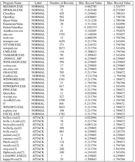
Program Name Label Number of Records Min. Record Value Max. Record Value REGMON.EXE NORMAL 259 -4.062785 -1.524777 SPOOLSS.EXE NORMAL 72 -5.422540 -0.272565 CloseKey NORMAL 429 -5.210662 -1.788163 OpenKey NORMAL 502 -4.828603 -1.758730 QueryValue NORMAL 594 -5.211228 -1.789106 EnumerateValue NORMAL 28 -3.311164 -1.542890 DeleteValueKey NORMAL 3 -5.1955757 -1.766465 AimRecover.exe NORMAL 61 -5.210285 -1.792879 aim.exe NORMAL 1702 -5.148589 -1.703827 ttssh.exe NORMAL 12 -4.860299 -1.794766 ttermpro.exe NORMAL 1639 -5.211794 -1.543456 NTVDM.EXE NORMAL 271 -4.234352 -1.794766 notepad.exe NORMAL 2673 -5.211794 -1.543456 CMD.EXE NORMAL 116 -5.388013 -1.794766 TASKMGR.EXE NORMAL 99 -3.309843 -1.543456 INS0432. MP NORMAL 443 -6.239865 -6.239865 WINLOGON.EXE NORMAL 399 -6.239865 -6.239865 systray.exe NORMAL 17 -6.239865 -6.239865 em exec.exe NORMAL 29 -6.239865 -6.239865 OSA9.EXE NORMAL 705 -5.211794 -1.789672 findfast.exe NORMAL 176 -5.211794 -1.794766 WINWORD.EXE NORMAL 1541 -5.211794 -1.789672 winmine.exe NORMAL 21 -1.794766 -1.794766 POWERPNT.EXE NORMAL 617 -5.211794 -1.543456 PING.EXE NORMAL 50 -5.211794 -1.789672 QueryKey NORMAL 11 -4.022096 -1.789672 wscript.exe NORMAL 527 -5.211794 -1.789672 AcroRd32.exe NORMAL 1598 -5.211794 -1.794766 0” NORMAL 404 -5.211794 -1.789672 WINZIP32.EXE NORMAL 3043 -5.211794 -1.789672 explore.exe NORMAL 108 -5.211794 -1.789672 EXCEL.EXE NORMAL 1782 -5.211794 -1.789672 bo2kss.exe[2] ATTACK 12 -4.022096 -1.789672

bo2k 1 0 intl.e[2] ATTACK 78 -5.211794 -1.789672 browselist.exe[4] ATTACK 32 -4.087124 -1.789672 bo2kcfg.exe[2] ATTACK 289 -6.239865 -6.239865 bo2k.exe[2] ATTACK 883 -6.239865 -5.245378 mstinit.exe[2] ATTACK 11 -6.239865 -6.239865 runonce.exe[2] ATTACK 8 -6.239865 -6.239865 Patch.exe[2] ATTACK 174 -5.211794 -1.789672 install.exe[3] ATTACK 18 -5.211794 -1.794766 xtcp.exe[3] ATTACK 240 -5.211794 -1.543456 l0phtcrack.exe[7] ATTACK 100 -4.194165 -1.543456 LOADWC.EXE[2] ATTACK 1 -6.239865 -6.239865 happy99.exe[5] ATTACK 29 -3.309843 -1.794766

Table 3. Information about test records for the second order polynomial kernel in the binary set-ting. The maximum and minimum discriminants are given, as well as the assigned classification label. Listed next to the attack processes is the attack source. [1] AIMCrack. [2] BackOrifice. [3] Backdoor.xtcp. [4] Browse List. [5] Happy 99. [6] IPCrack. [7] L0pht Crack. [8] Setup Trojan.

One-Class Training for Masquerade Detection

Ke Wang

Salvatore J. Stolfo

Computer Science Department, Columbia University

500 West 120

th

Street, New York, NY, 10027

{kewang, sal}@cs.columbia.edu

Abstract

We extend prior research on masquerade detection using UNIX commands issued by users as the audit source. Previous studies using multi-class training requires gathering data from multiple users to train specific profiles of self and non-self for each user. One-class training uses data representative of only one user. We apply one-class Naïve Bayes using both the multi-variate Bernoulli model and the Multinomial model, and the class SVM algorithm. The result shows that one-class training for this task works as well as multi-one-class training, with the great practical advantages of collecting much less data and more efficient training. One-class SVM using binary features performs best among the one-class training algorithms.

1. Introduction

The Masquerade attack may be one of the most serious security problems. It commonly appears as spoofing, where an intruder impersonates another person and uses that person’s identity, for example, by stealing their passwords or forging their email address. Masqueraders can be insiders or outsiders. As an outsider, the masquerader may try to gain superuser access from a remote location and can cause considerable damage or theft. A simpler insider attack can be executed against an unattended machine within a trusted domain. From the system’s point of view, all of the operations executed by an insider masquerader may be technically legal and hence not detected by existing access control or authentication schemes. To catch such a masquerader, the only useful evidence is the operations he executes, i.e., his behavior. Thus, we can compare one user’s recent behavior against their profile of typical behavior and recognize a security breach if the user’s recent behavior departs sufficiently from his profiled behavior, indicating a possible masquerader.

The insider problem in computer security is shifting the attention of the research and commercial community from intrusion detection at the perimeter of network systems. Research and development is going on in the area of modeling user behaviors in order to detect anomalous misbehaviors of importance to security; for example, the behavior of user-issued OS commands as represented in

this paper, and in email communications [17]. Considerable work is ongoing in certain communities to detect not only impersonation, but also author identification. For example, Sedelow [16] and Vel [18] are two examples bracketing the length of time this topic has existed in the literature.

The masquerade problem is a challenging problem. If the masquerader can mimic the user’s behavior successfully, he won’t be detected. In addition, if the user himself is behaving much differently than his trained profile, the detector will misclassify him as masquerader, which may cause annoying false alarms. There have been several attempts to solve this problem using command line sequences, [14] and [9]. The best results so far reported are 60-70% accuracy with a false positive rate as low as 1-2%. The profiles were computed using supervised machine learning algorithms that classify training data acquired from multiple user. These approaches considered training user profiles as a multi-class supervised learning task where data gathered on a user is treated as an example of one-class, i.e. a distinct user.

In this paper, we consider a different approach with substantial practical advantage. We examine the task of profiling a user by modeling his data exclusively, without using examples from other users, and achieving good detection performance and minimal false positive rates. We also consider alternative machine learning algorithms that may be employed for this “one-class” training approach.

One-class training means that we only use the user’s own legitimate examples of commands they issue to build the user’s self profile. Previous work uses both positive and negative examples to build both self and non-self profiles, except for Maxion [9], who considers the problem of determining how vulnerable a user’s behavior may be to mimicry attack. Here we extend this technique using one-class SVM. This is important in many contexts, especially when the only information available is the history of the user’s activities. If a one-class training algorithm can achieve similar performance to that exhibited by a multi-class approach, we may provide a significant benefit in real security applications; much less data is required, and training can proceed independently of any other user. The study reported in this paper indicates that indeed one-class training algorithms perform equally well as two class training approaches.

This self profile idea is similar to the widely used “anomaly detection” techniques in intrusion detection system [eg. 2, 3]. For example, the anomaly detector of IDES [8] uses established normal usage profiles, which is the expected behavior, to identify any large usage deviation as a possible attack. Several methods have been used to model the normal data, for example, decision trees [7], neural network [4], and sparse Markov Transducers [2], and Markov chains [19]. In this paper, we applied one-class Naïve Bayes and one-class SVM algorithms to the masquerade dataset of UNIX system call sequences.

In previous work, we believe there were several methodological flaws in the manner in which data was acquired and used. The “Schonlau dataset” from [14] presents each user’s command line data with a varying number of artificially created masquerade command blocks, ranging from 0 to 24, out of a total of 100 command blocks to be classified. The previous work only considered the average performance of a given method when it is applied to all of the 50*100 blocks of commands issued by the 50 users. However, since the masquerade blocks are “randomly” inserted into each user’s data by using some other user’s command block, each user’s data has a different number of masquerade blocks, and the content of these masquerade blocks all differ. This data is not a good baseline to compare the effectiveness of alternative detection methods because one method might be better at detecting certain forms of masquerade attack while others are not. Unfortunately, since the distribution of such masquerade blocks appear many times in the dataset, some algorithms appear to have better performance over others, while, in practice or in other contexts, this finding may not be true. To better compare the alternative methods proposed in this work, we follow the exhaustive “1v49” evaluation methodology from [9], which will be described in detail in the section about the experimental methodology and results. The ROC score [5] is used to compare several one-class training methods under different false positive rate restrictions. This approach provides a better view to indicate which algorithm is better for most users.

Even though one machine learning algorithm may perform better than another in terms of detection and false positive rate, our most important finding is that one-class training can indeed perform as well as multi-class training. Even so, the overall performance of both approaches indicates that there is much room for improvement.

The rest of the paper is organized as follows. Section 2 describes the dataset we used in our research and provides a review of recent work, and Section 3 discusses the one-class Naïve Bayes and one-one-class SVM methods. Section 4 describes the experimental setting and our results, and Section 5 concludes the paper with our analysis and findings.

2. Recent Work

Schonlau et al. [14] and Maxion [9] provide a dataset collected from keyboard commands on a UNIX platform. The dataset is publicly available at http://www.schonlau.net. Unfortunately, there are neither timestamps nor other detailed command line arguments available in the Schonlau dataset. Hence, the dataset in question consists simply of sequential “truncated” commands issued by each of 70 users. Each user is represented by 15,000 commands, collected over time from a few days to a few months. They randomly chose 50 users to serve as intrusion target, and the remaining 20 users as masqueraders. The first 5,000 commands of each user are “clean data” (legitimately issued by the user), and the next 10,000 commands of the target users were randomly injected with commands issued by the 20 masquerade users, apparently none of whom are any of the 50 users. The commands are grouped into blocks, with 100 commands per block. The commands in one block are either all clean or all masquerade attacks, called “dirty blocks”. The task studied in [14] is to accurately classify the “dirty” blocks as masquerade commands, while classifying the clean blocks as belonging to the user. From this point of view, this problem is very similar to a text classification problem, where the commands may be regarded as words or tokens in a document that is to be classified. Their work identifies six masquerade-detection schemes. They are: Bayes 1-Step Markov, Hybrid Multi-Step Markov, Incremental Probabilistic Action Modeling (IPAM), Uniqueness, Sequence-Match, and Compression. These masquerade detection methods were directly applied to this dataset; the first 5000 commands were used for training, and the remaining 10000 commands were inserted and used for testing, where each were processed in blocks of 100 commands. Testing and training were performed on a per block basis. The paper by Maxion [9] presents a clear and concise review of these six methods. The strategies behind each of these methods are quite different, but the results show that no method completely dominates another using cluster analysis and ROC curves.

Maxion [9] improved upon Schonlau’s result by applying the Naïve Bayes classification algorithm using the “bag of words” features. Naïve Bayes has been used in text classification for a long time and proved to be very efficient in this context as well. Naïve Bayes was also used in the earlier work [15] on classifying malicious code attachments in email messages. Maxion presents a detailed analysis of the origins of the classification error, revealing why some users are good masquerades and others are not. That paper designed another experiment, called “1v49”, to perform this error analysis. We also use the “1v49” experimental setting in our work, but here it is

used to compare the performance of different classifiers when applied to multiple classes.

The results for these reviewed methods are displayed in Table 1 and serve as a baseline for comparison.

Method Hits False Positives

N. Bayes (updating) 61.5% 1.5% N. Bayes (no Upd.) 66.2% 4.6% Uniqueness 39.4% 1.4% Hybrid Markov 49.3% 3.2% 1-step Markov 69.3% 6.7% IPAM 41.4% 2.7% Sequence Matching 36.8% 3.7% Compression 34.2% 5.0%

3. Machine learning methods

3.1. Learning task

For this masquerade detection problem, the learning task is to build a classifier that can accurately detect the masquerade commands while not misclassifying the user’s legitimate commands as a masquerade. Using the Schonlau dataset, which is organized as a set of blocks of 100 commands, the learning task is to compute a binary classifier whose input is a block of 100 commands and whose output is a classification of that block as either generated by a masquerader or not. The target classification is to detect the masquerader’s command blocks. Hence, the masqueraders’ data are positive examples, while the user’s legitimate data are treated as negative examples. Thus, a true positive outcome is a masquerade block of 100 commands, while a false positive outcome is a block of commands legitimately issued by the user but misclassified as a masquerade. In the following description, we call the masquerade blocks positive examples and call the legitimate blocks, those issued by the user himself, negative examples. One-class training means that a classifier is computed using only negative examples of the user himself as training data to build the classifier, which will be used to classify both positive and negative data. Thus, the task is to positively identify masqueraders, but not to positively identify a particular user.

3.2. One-class or two class

Previous work considered the problem as a multi-class supervised training exercise. The dataset contains data for 50 users. For each user, a specific class, the first 5000 commands are treated as negative examples, while the data from the other 49 users are treated as positive examples. It is reasonable to assume the negative examples, which belong to the same user, were treated consistently, while the positive examples used in training belong to another user. For the masquerade problem, it is probably impossible and unreasonable to estimate how an attacker would behave. Thus, treating sets of other users’ data as positive examples provides a substantive bias (to those users’ behavior who probably was not behaving maliciously). We next present the means of implementing one-class training for Naïve Bayes classifier and for SVM, using only data from a single user when training a classifier to profile a distinct user.

3.3. Naïve Bayes Classifier

The Naïve Bayes classifier [12] is a simple and efficient supervised learning algorithm, which has been proved to be very effective in text classification, and many other applications. It is based on Bayes’ rule,

) ( ) | ( ) ( ) | ( d p u d P u p d u p =

which calculates the probability of a class given an example. Applied to the masquerade problem, it calculates the likelihood that a command block belongs to a masquerader (non-self), or some legitimate user. Different commands

c

_i , which are used as features here, are assumed independent from each other. This is the Naïve part of this method.

There are two common models used in Naïve Bayes Classifier, one is the multi-variate Bernoulli model, and the other is the multinomial model [11]. In the multi-variate Bernoulli event model, a vector of binary attributes is used to represent a document (in our case, a block of 100 commands), indicating whether the command occurs or doesn’t occur in the document. The multinomial model uses the number of command occurrences to represent a document, which is called “bag-of-words” approach, capturing the word frequency information in documents. According to McCallurn [11]’s result, multi-variate Bernoulli model performs better for small vocabulary size, and the multinomial model usually performs better at larger vocabulary size. Because the vocabulary size (the number of distinct commands) of this masquerade problem is 856, which is a moderate in size, we want to compare both of these models for this problem.

Multi-variate Bernoulli model

Using the multi-variate Bernoulli Model, a command block d is represented as a binary vectord=(b1(d),b2(d),...,bm(d))

→

, with

b

_i

(d

)

set to 1 if the command

c

_i occurs at least once in this block. Here

m

is the total number of features, i.e., the number of distinct commands. Given p(ci|u) , which is the

probability estimated for command

c

_ifor user

u

in the training data, we can compute

p

( u

d

|

)

of the test block

d as: = ) | ( ud p ) )) | ( 1 ))( ( 1 ( ) | ( ) ( ( 1

∏

= − − + m i i i i i u c p d b u c p d b (1)

where p(ci |u)is estimated with a Laplacean prior: ) ( 2 ) , ( 1 ) | ( u N u c N u c p i i ₊ + = (2)

)

(u

N

is the number of training examples for user

u

, while

N

( u

c

i

,

)

is the number of documents containing the command

c

_i for user

u

.

Multinomial model

Using the standard bag-of-words approach, each command block is represented by a feature vectord=(n1(d),n2(d),...,nm(d))

→

, where

n

_i

(d

)

is the number of times command

c

_iappears in the command blockd. Similarly, givenp(ci|u), which is the frequency

count computed for command

c

_ifor user u in the training data, we can compute

p

( u

d

|

)

of the test block d as:

∏

=

=

m i d n i

u

i

c

p

u

d

p

1 ) (

))

|

(

(

)

|

(

(3)

where

p(c_i|u)

is derived from:

m

d

n

d

n

u

c

p

_m i u N j i j u N j i j i

*

)

(

)

(

)

|

(

1 ) ( 1 ) ( 1

α

α

+

+

=

= = =

(4)

Here

α

is used for smoothing, which controls the sensitivity to previously unseen commands. (This implies there is a non-zero probability any command may be issued by any user.) We set it to 0.01 following [9].

One-class Naïve Bayes

Adapting the above algorithm to one-class Naïve Bayes, which uses only positive examples for training, is very simple. We only compute

p

(

c

_i

|

u

)

for useru’s self profile. For the non-self profile, we can assume each

command has equal probability m1/ , which is essentially random. Thus, given a test d , we can compare

)

|

(

d

self

p

with

p

( nonself

d

|

)

. The larger the ratio of

)

|

(

d

self

p

to

p

( nonself

d

|

)

, the more likely this command block d is from the user

u

.

Applying the one-class Naïve Bayes algorithm to our specific dataset is also quite simple. Since each test document (a block of commands) has a fixed number of 100 commands, the probability of “non-self” is the same for all tested blocks. Since we do not have to compute the probability of non-self; we may compare the probability of being “self” to a threshold in order to decide whether this block is a masquerade block or not. Furthermore, we can easily adjust the threshold to control the false positive and detection rate.

3.4. One-class support vector machine

Support Vector Machines (SVM) have been shown to be highly effective in text classification as well [6], among other important learning tasks. They are maximal-margin classifiers, rather than probabilistic as is Naïve Bayes. In the two-class formulation, the basic idea is to map feature vectors to a high dimensional space and to compute a hyperplane that not only separates the training vectors from different classes, but also maximizes this separation by making the margin as large as possible.

Scholkopf et al. [13] proposed a method to adapt the SVM algorithm for one-class SVM, which only use examples from one-class, instead of multiple classes, for training. The one-class SVM algorithm first maps input data into a high dimensional feature space via a kernel function and treats the origin as the only example from other classes. It then iteratively finds the maximal margin hyperplane that best separates the training data from the origin.

Considering that our training data setx1,x2,...,x ∈X,

Φ is the feature mapping X →F to a high-dimensional space, we can define the kernel function as:

))

(

)

(

(

)

,

(

x

y

x

y

k

=

Φ

⋅

Φ

Using kernel functions, the feature vectors need not be computed explicitly, greatly improving computational efficiency since we can directly compute the kernel values and operate on their images. Some common kernels are linear, polynomial, and radial basis function (rbf) kernels: Linear Kernel:

k

(

x

,

y

)

=

(

x

⋅

y

)

P-th order polynomial kernel:

k

(

x

,

y

)

=

(

x

⋅

y

+

1

)

p rbf kernel:

k

(

x

,

y

)

=

e

−||x−y||2/2σ2

Now, solving the one-class SVM problem is equivalent to solving the dual quadratic programming (QP) problem:

ij i j i j

x

x

k

(

,

)

2

1

min

_α

α

α

subject to

₀

≤

≤

1

,

=

1

.

i i i

v

α

α

where

α

_i is a Lagrange multiplier, which can be thought of as a weight on example

x

_i, and

ν

is a parameter that controls the trade-off between maximizing the number of data points contained by the hyperplane and the distance of the hyperplane from the origin.

After solving for

α

_i, we can use a decision function to classify data. The decision function is:

−

=

_i i

k

x

i

x

x

f

(

)

sgn(

α

(

,

)

ρ

)

where the offset

ρ

can be recovered by

) , ( j i j jk x x =

α

ρ

.

In our work, we used the LIBSVM 2.4 [1] available at http://www.csie.ntu.tw/~cjlin/libsvm for our experiments. LIBSVM is an integrated tool for support vector classification and regression that implemented Sholkopf’s algorithm for one-class SVM. We used the default rbf kernel and the default values of the parameters for one-class SVM.

Another problem to consider for one-class SVM is how to represent the features. We used both a word count representation and a binary representation, which are equivalent to the multinomial model and multi-variate Bernoulli model of Naïve Bayes algorithm, respectively. The vectors are normalized to length 1.

4. Evaluation

We conducted two sets of experiments. The first experiment repeats the experimental methodology of [14]. We show that the performance of one-class training is almost the same as the performance of multi-class training. This is a significant finding on its own.

The second experiment aims to compare the performance of the two one-class training algorithms when applied to multiple users. Following [9], we will call the first the SEA experiment, which is from the authors’ names in [14], Schonlau et al. The second experiment is

called 1v49, because we trained using only one user’s data and tested on all other 49 user’s data.

4.1. SEA Experiment

Recall that in this experiment, the first 5,000 commands of a user serve as positive examples, and the first 5,000 commands of all the other 49 users serve as negative examples. The resultant classifier is tested on the rest of the 10,000 commands of the user. These have

inserted “dirty” command blocks under a probability distribution from other users besides the 50 users whose commands were trained on. For our one-class algorithm, the test data remains the same, but we only use one user’s training data (the first 5,000 commands) as negative examples for training; there are no positive examples used at all to compute the classifier. First we compare the Naïve Bayes classifier using the multi-variate Bernoulli model and the multinomial model. Then we compare the one-class training algorithms against the multi-class training algorithms. All the classification algorithms we tested do no updating during the test of any parameters because we want to compare the pure performance of each of them. Maxion [9] used an empirically pre-fixed threshold to update the classifier during the experiment, which is not an intrinsic characteristic of the classification algorithm. ! " ! " ! " ! " !!!!

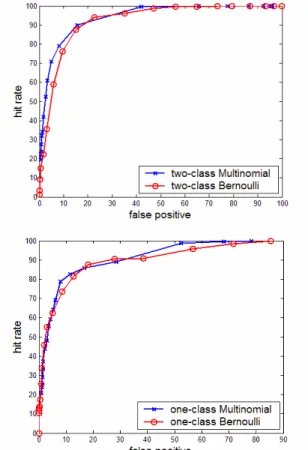
Figure 1 displays plots comparing the multi-variate Bernoulli model and the multinomial model of Naïve Bayes classifier. When using multi-class training, the multinomial model is obviously better than the Bernoulli model. But the difference is not so obvious in one-class training, especially when the false positive rate is low. We

thus compare both models in the following 1v49 experiment.

To compare the performance of the one-class training algorithms against the multi-class training algorithm on the same test data, we plot the ROC curves as displayed in Figure 1. For the multi-class training algorithm, we only use the multinomial model Naïve Bayes algorithm as the baseline for comparison, which is better than Bernoulli model and has been proved to the best among the variety of methods as described in [9]. For the one-class SVM, we compare both the binary and word count representations. From Figure 2, we can see that only one-class SVM using the word count representation is a little bit worse than the other three methods. One-class SVM using the binary representation and one-class Naïve Bayes achieved almost the same performance as the two class Naïve Bayes algorithm.

We also compare in Figure 3 the performance of all the previous algorithms from Table 1 to one-class SVM algorithm using binary features, which is best one among the one-class training algorithms. One-class SVM-binary is better than most of the previous algorithms except the two-class multinomial Naïve Bayes algorithm with updating.

This experiment confirmed our conjecture that for masquerade detection, one-class training is as effective as two class training.

#### $ % & ' $ % & ' $ % & ' $ % & ' (((( $ ) *$ ) *$ ) *$ ) *

4.2. 1v49 Experiment

As we have pointed out, since the dataset used had randomly inserted masquerade blocks in each user’s test commands (10,000 commands following the first 5,000), each user has a different number of “dirty” blocks and the origins of these “dirty” blocks also differ. So the result of the SEA experiment may not illustrate the real performance of a classification algorithm. (There are too many unfixed parameters.) To better evaluate the performance of a classification algorithm, we can treat these 50 users as our selected sample of common users. If we can prove algorithm A is better than algorithm B for most of the 50 users, we can infer A is better than B in a general sense.

To meet this requirement, we follow the “1v49” experiment, but for a different purpose. We use one user’s first 5,000 commands as negative training data to compute a classifier without any positive training data. For test data, we use the non-masquerade blocks from the 10,000 additional commands of the same user as negative test data, and the other 49 users’ first 5,000 commands as positive test data. This data is also organized in blocks of 100 commands.

As we mentioned before, the same algorithm might perform quite differently for different users. Figure 4 illustrates the difference. Figure 4 shows the ROC curve for user 2, 20 and 40 using one-class SVM with the binary feature representation. Such a difference occurs no matter which algorithm has been used; the difference is determined by the characteristic of each user.

+ , + ,+ , + , $ ) * $ ) * $ ) * $ ) *

To compare the different methods for multiple users, we compute the ROC score for each user. In general, a ROC score is the fraction of the area under the ROC curve, the larger the better. A ROC score of 1 means perfect detection without any false positives. Figure 5 below shows the ROC scores for users 20 and 40 using the one-class SVM-binary algorithm

.

- , % ' # . - , % '- , % ' # .# . - , % ' # . + . , + . , + . , + . ,

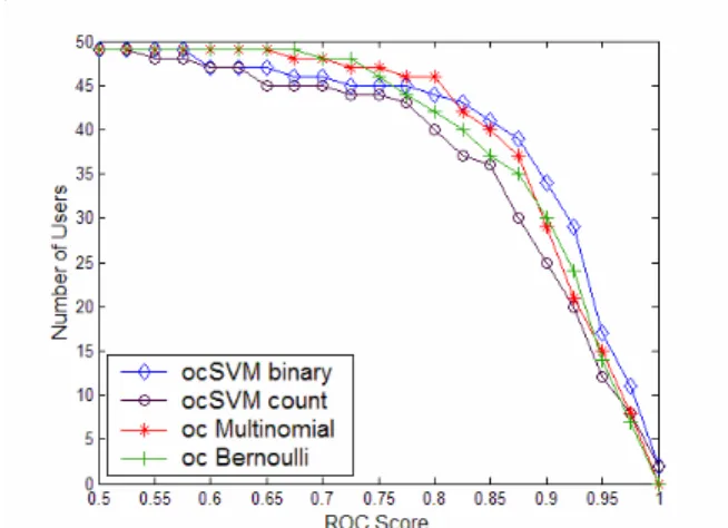
Figure 6 illustrates the performance of several one-class training algorithms as measured by ROC scores. The figure includes results for all 50 users. From Figure 6, we can see that one-class SVM using word-count features is the worst among the four algorithms. At the high ROC score region, with a ROC score higher than 0.8 (which is what we prefer) one-class SVM using binary features performs best among all. There is no big difference between Naïve Byaes using the multinomial model or the multi-variate Bernoulli model.

/ , 0 / ,/ , 00 / , 0 " ' " ' " ' " '

For the masquerade problem, we are more interested in the region of the ROC curve with a low false positive rate; otherwise, the “annoyance level” of false alarms would render the detector useless in practical use. Therefore, we restrict the ROC scores to the curves with false positive lower than P, which is called the ROC-P score. For example, if we want to restrict the false positives to be lower than 5% of all command blocks, we can compute ROC-5. Similar to the general ROC score, the ROC-P score is the fraction of the area under the ROC curve where the false positive rate is lower than P%. Figure 7, displays an example of 10, based on the ROC-curves of users 20 and 40. Only part of the ROC curve is drawn here to highlight the plots.

1 , 1 , 1 , 1 , .... # .# .# .# . + . ! "+ . ! "+ . ! "+ . ! " 2 3 . 4 2 3 . 42 3 . 4 2 3 . 4

Since we can see that one-class SVM using the binary feature is generally better than one-class SVM using the word count feature, as depicted in Figure 6; here we only compare the one-class SVM using the binary representation with the multinomial model Naïve Bayes and Bernoulli model Naïve Bayes in the following ROC-P comparison. Figures 8 plots the co