Power System Reliability Analysis with Distributed Generators

Power System Reliability Analysis with Distributed Generators

by Dan Zhu

Thesis submitted to the faculty of

Virginia Polytechnic Institute and State University in partial fulfillment of the requirements for the degree of

Master of Science In

Electrical Engineering

Approved:

Dr. Robert P. Broadwater, Chairman

Dr. Ira Jacobs Dr. Timothy Pratt

May, 2003 Blacksburg, VA

Power System Reliability Analysis with Distributed Generators

Dan Zhu

Committee Chairman: Dr. Robert P. Broadwater, Electrical Engineering

Abstract

Reliability is a key aspect of power system design and planning. In this research we present a reliability analysis algorithm for large scale, radially operated (with respect to substation), reconfigurable, electrical distribution systems. The algorithm takes into account equipment power handling constraints and converges in a matter of seconds on systems containing thousands of components. Linked lists of segments are employed in obtaining the rapid convergence. A power flow calculation is used to check the power handling constraints. The application of distributed generators for electrical distribution systems is a new technology. The placement of distributed generation and its effects on reliability is investigated. Previous reliability calculations have been performed for static load models and inherently make the assumption that system reliability is independent of load. The study presented here evaluates improvement in reliability over a time varying load curve. Reliability indices for load points and the overall system have been developed. A new reliability index is proposed. The new index makes it easier to locate areas where reliability needs to be improved. The usefulness of this new index is demonstrated with numerical examples.

Acknowledgements

I would like to acknowledge the invaluable guidance, concern and support of my advisor, Dr. Robert Broadwater. During this research, he always accepted my ideas with an open mind and gave me the maximum opportunity to contribute to the program. His advice really helped me to refine the application.

I would like to thank Electric Distribution Design (EDD) Inc. for providing facilities to finish this research work, and Electric Power Research Institute (EPRI) Distribution Engineering Workstation (DEW) for benchmark analysis of the power flow calculations.

Thanks are also due to Dr. Jacobs and Dr. Pratt for serving on my committee. They both helped to review my thesis paper.

My husband, Max, deserves special thanks. His unselfish support and encouragement has allowed me to keep my perspective during this time.

Table of Contents

1. Introduction ………... 1

1.1. Introduction ………... 1

1.2. Objective of the Research ……… 1

1.3. Distributed Generators……….. 2

1.4. Literature Review ………. 3

1.5. Definition of Power System Reliability……… 4

1.6. Reliability Assessment Techniques……….. 5

2. Measuring Service Quality……….. 7

2.1. Definitions of Performance Indices……….. 7

3. Comparison of Different System Designs……….. 9

3.1. Simple Radial Distribution System……… 9

3.2. Alternative Feed Distribution Arrangement………..10

3.3. Alternative Feed Arrangement with DR ……….. 10

4. Switching Operations………... 12

5. Reliability Analysis Sets………... 14

5.1. Segment………... 14

5.2. Reliability Analysis Sets………... 15

6. Pointer and Circuit Traces………... 21

6.1. Workstation Circuit Model………...21

6.2. Pointers………... 22

6.3. Circuit Traces………... 24

7.3 Power Flow Calculation………. 36

7.4 Software Design………. 38

8. Reliability Indices ……….42

8.1. Functional Characterization………... 42

8.2. Reliability Indices Calculation………... 43

8.3. Relative Reliability Index………... 45

9. Distributed Generator Placement ………... 48

10. Case Studies………... 49

10.1. Introduction………. 49

10.2. Case Study One……….. 49

10.3. Case Study Two……….. 58

10.4. Case Study Three……… 61

11. Conclusions and Further Research………... 65

11.1. Conclusions……… 65

11.2. Further Research………. 66

12. References ………... 67

Appendix A ………... 69

List of Figures

Figure 1.1 Subdivision of System Reliability………...5

Figure 3.1 Simple Radial Distribution System………...9

Figure 3.2 Alternative Feed Distribution Arrangement ………...10

Figure 3.3 Alternative Feed Arrangement with DR ………...11

Figure 4.1 Sample Circuit………...………...13

Figure 5.1. Sample segment ………...………....15

Figure 5.2. Reliability Analysis Sets ………...………..16

Figure 6.1 Sample Circuit ………...………...25

Figure 7.1 Illustrating Selection of Alternative Feed ………...34

Figure 7.2 Reliability Analysis Algorithm Sequence Diagram ………39

Figure 8.1 Example Circuit for Relative_CAIDI ………...46

Figure 10.1 System 1 for Case Study One ………...50

Figure 10.2 System 2 for Case Study One: Adding an Alternative Feed ….53 Figure 10.3 System 3 for Case Study One: Adding a Distributed Generator ………...………...…...56

Figure 10.4 System for Case Study Two ………...…………58

Figure 10.5 Addition of Substation and DG to System Shown in Figure 10.4 ………...………... 59

Figure 10.6 DG at the End of Circuit ………...………..60

Figure 10.7 Circuit for Case Study Three ………...62

Figure 10.8 Down Time Variation with Varying Load of L_C32 ……….. 63

List of Tables

Table 6.1 DEW Component Trace Structure Element ………23 Table 7.1 Summary of Traces Used to Develop the RA Sets ………..36 Table 7.2 Summary of Messages in the RA Sequence Diagram ………….40 Table 10.1 Equipment Index Table ………..………51 Table 10.2 Improvement of Reliability ………..………..55 Table 10.3 Comparison of Reliability Improvements ………..57 Table 10.4 System Reliability Improvement for Case Study Two ……….. 61

1. Introduction 1.1. Introduction

The economic and social effects of loss of electric service have significant impacts on both the utility supplying electric energy and the end users of electric service. The cost of a major power outage confined to one state can be on the order of tens of millions of dollars. If a major power outage affects multiple states, then the cost can exceed 100 million dollars. The power system is vulnerable [1] to system abnormalities such as control failures, protection or communication system failures, and disturbances, such as lightning, and human operational errors. Therefore, maintaining a reliable power supply is a very important issue for power systems design and operation.

This thesis presents the research efforts and the software implementation of a reliability analysis algorithm for electrical power distribution systems. This algorithm is used to study reliability improvements due to the addition of distributed generators. This algorithm also takes into account system reconfigurations.

1.2. Objective of the Research

One objective of this research is to evaluate power system reliability analysis improvements with distributed generators while satisfying

power system reliability. This algorithm needs to converge rapidly as it is to be used for systems containing thousands of components. So an efficient “object-oriented” computer software design and implementation is investigated.

This algorithm is also used to explore the placement of distributed generators and how the different placements affect system reliability, which has not been done in previous research. This exploration makes possible the comparison of alternative system designs to discover systems yielding desired reliability properties.

In this paper, variation of power system reliability with the varying loads is also investigated. Other publications of distribution system reliability analysis associated with time varying loads have not been found.

1.3. Distributed Generators

Distributed generators (also known as Distributed Resources) come in many forms including gas turbine driven synchronous generators, wind powered induction generators, fuel cells with inverter circuitry, and others. The use of distributed resource generation is projected to grow. This growth is due to cost reductions available with distributed generators. The cost reductions may be the result of released system capacity or reductions in generation costs at peak conditions.

1. 4. Literature Review

Prior to the 1960’s, the reliability of proposed power systems was often estimated by extrapolating the experience obtained from existing systems and using rule-of-thumb methods to forecast the reliability of new systems[3].

During the 1960’s considerable work was performed in the field of power system reliability and some excellent papers were published. The most significant publications were two company papers by a group of Westinghouse Electric Corporation and Public Service and Gas Company authors[3],[4]. These papers introduced the concept of a fluctuation environment to describe the failure rate of transmission system components. The techniques presented in these papers were approximations which provided results within a few percent of those obtained using more theoretical techniques, such as Markov processes. The application of Markov Chains in the power system reliability field was illustrated in Reference [5]. The Markov approach is limited in application because of computer storage requirements and the rounding errors which occur in the solution of large systems.

Most previous publications have focused on transmission system reliability. This research focuses on distribution system reliability. This work extends previous research[5], which demonstrated sets used in describing power system reliability calculations. Reference [6] presented the first

took into account constraints associated with switching operations, but it was relatively slow due to running numerous power flow calculations.

One aspect investigated h ere is the effect of Distributed Generators (DG) on power system reliability. Standards for connecting DGs into distribution systems are just being developed. Reference [7] deals with issues related to existing DG interconnection practices. An investigation of eleven utilities and industry interconnection standards was performed to identify the key requirements for a DG connection. The results of this investigation led to the development of a unified approach for determining interconnection requirements. Reference [8] considers many aspects of DGs in distribution systems, including protection, harmonics, transients, voltage and frequency control. A Power flow calculation based on the positive sequence model of the distribution circuits was presented.

1.5. Definition of Power System Reliability

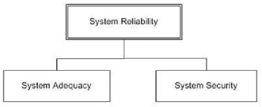
The function of an electric power system is to satisfy the system load requirement with a reasonable assurance of continuity and quality. The ability of the system to provide an adequate supply of electrical energy is usually designated by the term of reliability. The concept of power-system reliability is extremely broad and covers all aspects of the ability of the system to satisfy the customer requirements. There is a reasonable subdivision of the concern designated as “system reliability”, which is shown in Figure 1.

Figure 1.1 Subdivision of System Reliability

Figure 1 represents two basic aspects of a power system: system adequacy and security. Adequacy relates to the existence of sufficient facilities within the system to satisfy the consumer load demand. These include the facilities necessary to generate sufficient energy and the associated transmission and distribution facilities required to transport the energy to the actual consumer load points. Security relates to the ability of the system to respond to disturbances arising within that system. Security is therefore associated with the response of the system to perturbations[9]. Most of the probabilistic techniques presently available for power-system reliability evaluation are in the domain of adequacy assessment. The techniques presented in this paper are also in this domain.

1.6 Reliability Assessment Techniques

Reliability analysis has a wide range of applications in the engineering field. Many of these uses can be implemented with either qualitative or

Quantitative methodologies use statistical approaches to reinforce engineering judgments. Quantitative techniques describe the historical performance of existing systems and utilize the historical performance to predict the effects of changing conditions on system performance. In this research, quantitative techniques combined with theoretical methods are used to predict the performance of designated configurations. The systems considered in this research are radially operated[10] with respect to substations, but are reconfigurable.

2. Measuring Service Quality – Performance Indices

A basic problem in distribution reliability assessment is measuring the efficacy of past service. A common solution consists of condensing the effects of service interruptions into indices of system performance. The Edison Electric Institute (EEI), the Institute of Electrical and Electronics Engineers (IEEE), and the Canadian Electric Association (CEA) have suggested a wide range of performance indices[11]. These indices are generally yearly averages of interruption frequency or duration. They attempt to capture the magnitude of disturbances by load lost during each interruption.

2.1. Definitions of Performance Indices

SAIDI (system average interruption duration index) is the average interruption duration per customer served. It is determined by dividing the sum of all customer interruption durations during a year by the number of customers served. customers of number total durations erruption int customer of sum SAIDI =

CAIDI (customer average interruption duration index) is the average interruption duration for those customers interrupted during a year. It is determined by dividing the sum of all customer interruption durations by the number of customers experiencing one or more interruptions over a one-year period. erruptions int customer of number total durations erruption int customer of sum CAIDI =

These two performance indices express interruption statistics in terms of system customers. A customer here can be an individual, firm, or organization who purchases electric services at one location under one rate classification, contract or schedule. If service is supplied to a customer at more than one location, each location shall be counted as a separate customer.

3. Comparison of Different System Designs

Of paramount interest in any reliability study is ensuring a good quality of service to customers defined as a combination of availability of the energy supply and the quality of the energy available to the customers (Medjoudj, 1994). In the following sections we will discuss the reliability of the power supply for three kinds of situations. We will show how reconfiguration and alternative sources improve the reliability of the power system.

3.1. Radial Distribution System

Figure 3.1 shows a simple Radial Distribution System. In this system a single incoming power service is received and distributes power to the facility.

Figure 3.1 Simple Radial Distribution System

There is no duplication of equipment and little spare capacity is typically included. Failure of any one component in the series path between

3.2. Alternative Feed Distribution Arrangement

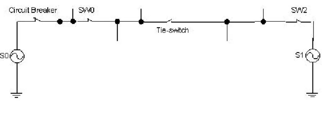
A second distribution arrangement is used for facilities requiring more reliable power. Figure 3.2 is a diagram representing this system arrangement. Part of the load is connected to one source and the other part of the load is connected to a second power source.

Figure 3.2 Alternative Feed Distribution Arrangement

The circuits (one circuit fed by S0 and the other fed by S1) are tied together through a normally open tie-switch, with both power sources energized. The electrical equipment is designed to accommodate 100% of the facility load. For instance, when a failure occurs in source S0, after the failure is isolated by opening the circuit breaker, the tie-switch is closed allowing the complete load to be served from a single source until the problem is corrected. Most customers can be restored immediately and don’t have to wait until S0 is repaired.

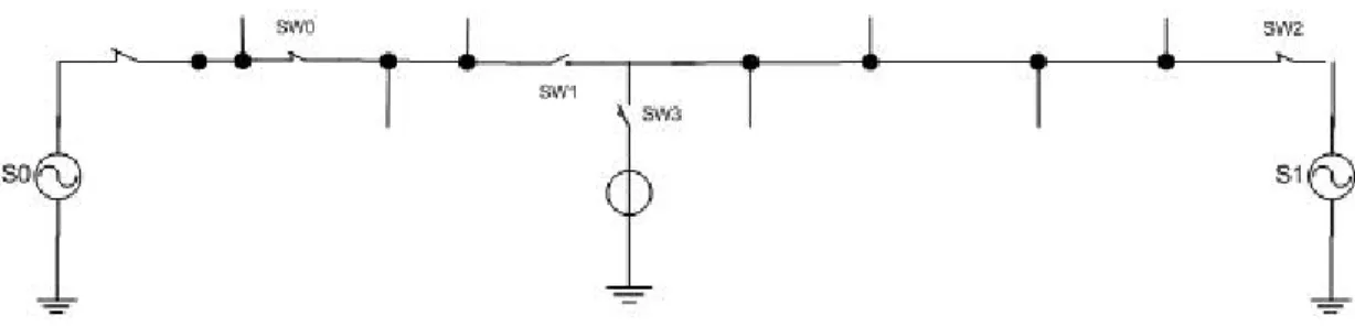
3.3. Alternative Feed Arrangement with DR

the left hand side of SW0, we can open SW0 and close SW3, so that the DR can pick up the rest of the circuit, which was originally fed by S0. Without the DR, we have to draw the power from S1. Such operation might violate system constraints or degrade the quality of the power supply, especially when the customer load reaches a peak value.

4. Switching Operations

Reliability analysis for a power system also leads to more reliable and cost-effective operation, since power restoration analysis is a subset of the calculations performed for reliability analysis. Here we assume switch operation time is less than repair time, so loads that have lost power may be restored faster by appropriate switching operations, or reconfiguration of the system.

There are two kinds of switching operations of interest. One is isolating the failure point so that a load point of interest which has lost power may be re-supplied from the original source. The other is to again isolate the failure point and to feed a load point of interest from an alternate source, if an alternate source is available. For example, in Figure 4.1, if a fault happens in component 5, we can open switch SW4 to isolate component 5 from the rest of the system. The original source S0 can still supply power to all the customers, except those on the downstream of switch SW4.

Figure 4.1 Sample Circuit

The second kind of switching operation isolates the failure point and interrupts the original power supply to the load point of interest. In this case we need an alternate feed to restore power to the load point of interest. For instance, if component 2 in the example circuit has a permanent fault, the fault can be isolated by opening B1 and SW14. In case there is no alternate source, all the segments downstream of the failed zone can only be restored after the fault is repaired. Since we have an alternate source S1 (assuming S1 can supply the power and the alternative feed path can carry the power), downstream of SW14 can be restored by closing SW25. The restoration time for this part of the system is shorter with switching operations than with the

5. Reliability Analysis Sets 5.1. Segment

In essence, there are two configurations in a distribution system. One consists of lines, transformers, and other components that are directly responsible for transmitting power from the distribution substation to customers. The second one consists of fuses, reclosers, circuit breakers, etc. This interrelated network is designed to detect unusual conditions on the power delivery system and isolate the portions of system that are responsible for these conditions from the rest of the network. The location of protection or isolation components on the distribution system and their response to failures can have an important impact on the reliability indices. We will sectionalize the distribution system into segments by these protection and isolation components. In the following pages, the power system is not modeled in terms of components but segments. A segment is a group of components whose entry component is a switch or a protective device. This sectionalizing device isolates groups of components into indivisible sections. Each segment has one and only one switch or protective device.

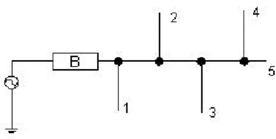
In Figure 5.1, the only protection on the feeder is the station breaker. The failure of any of the components in this segment can cause an interruption at load point 1. It is the same for the other load points (2, 3, 4, and 5). No temporary restoration is possible. For this configuration, the reliability of all the load points (1, 2, 3, 4, and 5) is identical.

Figure 5.1. Sample segment

A segment’s name is the same as that of its sectionalizing device. In Figure 5.1, there is only one segment, which is segment B. Breaker B and components 1, 2, 3, 4 and 5 all belong to segment B.

Modeling the power system in terms of segments speeds up the reliability index calculations. The algorithm can be programmed to run faster since only the sectionalizing devices are processed without processing the intermediate components.

5.2. Reliability Analysis Sets

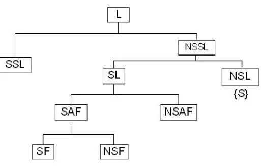
In order to analyze the reliability of distribution systems, the Electric Power Research Institute (EPRI) defined sets [11] needed for calculating the reliability of a given load point. Figure 5.2 illustrates the relation among these sets.

Figure 5.2. Reliability Analysis Sets

In reliability analysis, the failure of all elements that can cause a loss of service to a particular load point must be considered. (This load point will be presented in terms of a segment, which is the segment of interest S.) All system components are either located on the continuous path between the source and the segment of interest, or not located on the path. The failure of all continuous path components can cause an interruption at the load point. And the failure of components not in the path can also cause an interruption at the load point, unless the component is separated from the path by a protective device that responds automatically to the component failure. The effects of nonseries elements and temporary restoration are now considered in the sets shown in Figure 5.2, as will now be explained.

The L set shown in Figure 5.2 contains all segments within a circuit whose failure can cause loss of power to the segment of interest S. This L set includes all segments that are not separated from the continuous path between the source (substation, generator, etc.) and the segment of interest S

by an automatic protection device.

Now we partition the L set into the sets SSL and NSSL:

• The SSL set consists of the segments that may be isolated from the continuous path between S and the original source

• The NSSL set consists of the segments that cannot be switched away from the continuous path between S and the original source.

The SSL set contains any segments separated from the continuous path by manually operated switches. If any element of this set fails, the segment of interest S can be temporarily restored from the original source before the failed component is repaired or replaced.

Examining those segments that cannot be separated from the continuous path, we can further partition the set NSSL into SL and NSL:

• The SL set consists of the segments that can be switched away from the segment of interest S, so that if the failure occurs in the SL set, S may be fed by an alternate source

• The NSL set consists of the segments that cannot be switched away from the segment of interest S. That is the segment of interest itself, so this set only contains the element {S}.

If any thing fails in the NSL set, all the components within that segment have to experience the full repair or replacement time of the failed component. Temporary restoration is not possible.

Considering the SL set, we can divide it into SAF and NSAF:

• For the SAF set, if the failed component lies in these segments, it is possible to restore power to S by an alternate source

• For the NSAF set, if the failed segment belongs to this set, the segment of interest S cannot be temporarily restored from an alternate feed.

The set SAF contains the segments that can be isolated from both the segment of interest S and the alternative source, which make the temporary restoration topologically possible. Sometimes, system constraints may limit the restoration options; the alternate source might not have the capacity to support the particular load point that of interest. So the set SAF is partitioned into SF and NSF:

alternative source (for segments in this set, system constraint violations do not occur during the restoration)

• The NSF set consists of all segments which may be isolated from S and an alternative source, but for which it is not possible to restore power to S because of violating system constraints.

The set L, including all the segments for calculating the reliability indices, is decomposed into a number of sets as given by

L=SSL∪NSSL; (5.1) NSSL=SL∪{S}; (5.2)

SL= SAF∪NSAF; (5.3)

SAF= SF ∪NSF (5.4)

Equation (5.1), (5.2), (5.3) and (5.4) yield

L=SSL∪SF∪{S} ∪NSAF∪NSF (5.5) To sum up, if the failed component from the L set is placed in the SSL

set, it is possible to restore power to the load point of interest S from the original source. If the failure occurs in the SF set, the power can be restored

the failed component locates in either {s}, NSAF or NSF sets, then the failed component must be completely repaired before power can be restored to S.

We use several additional reliability analysis (RA) sets to calculate the sets of Equation (5.5), as given by

SIC = a set of all the segments in the circuit

SW = a set of all the sectionalizing devices in the circuit AF = a set of available alternate sources

IS = a set of sectionalizing devices that will isolate the segment of interest S from the original sources

NIS = a set of switches that do not isolate the original source from the segment of interest

EC = a set of ending components for the circuit

PD = a set of protective devices in the circuit that isolate a load point of interest from its source.

6. Pointer and Circuit Traces 6.1. Workstation Circuit Model

Electric Power Research Institute’s Distribution Engineering Workstation, DEWorkstation, provides an engineering environment that is focused on the design and analysis of electric distribution systems[12]. DEWorkstation is used in the research here.

Reliability analysis is complicated by a number of factors. One of these is the size of distribution systems. Large metropolitan areas may contain thousands of devices with several separate circuits supplied by different substations. Calculation of reliability for a system is an extensive logistical problem. Fundamental to reliability improvement is manipulation of large amounts of interrelated data. This data includes distribution system configuration, system fault protection, customer density, failure rate and repair time. The methods with which this data is stored, displayed and modeled determine the effectiveness of the computerized method. In DEWorkstation, information about the distribution system under study is permanently stored in data base tables. Initialization of the environment results in the most commonly used circuit model data being loaded into the workstation active memory[13]. This data is immediately available to and shared by application modules, such as the reliability analysis application. In this way, the number of accesses to the relational database is minimized. The most commonly used application modules run entirely in high speed memory and do not have to access the hard disk. This approach provides

6.2. Pointers

With large amounts of data in active memory, data structure manipulation is a primary concern. A feature of the C language which has a significant impact on this problem is the pointer. The pointer is a variable that holds the address of a data element. Pointers permit the construction of linked lists of data elements in computer memory [14]. In DEWorkstation, pointers are used for all data objects. Applications share circuit information via pointers, and also use pointers to manipulate data objects hidden inside the applications.

In distribution systems, a single circuit model may contain over 5000 components, and an entire system model consisting of hundreds of circuits may contain over a million components. With such large systems, modeling methods have a direct impact on the ability to perform engineering analysis. Use of pointers in linked lists allows system interconnects and equipment parameters to be directly available for analysis without repetitive search algorithms. Intrinsic in the graphical creation of the circuits is the creation of linked lists. The DEWorkstation memory model links together sources and components of each circuit[15]. In this way, it is possible to trace from circuit to circuit, through an individual circuit, or through a particular branch of a circuit.

Application programmers work with DEWorkstation defined objects. These objects are manipulated and accessed via pointers and indices into arrays of pointers. The links provided that pertain to component traces

• Forward Pointer—forward direction for doubly linked list of circuit components

• Backward Pointer— backward direction for doubly linked list of circuit components

• Feeder Path Pointer — for a radial system, the feeder path pointer of a given component is the next component toward the reference substation that feeds the given component

• Brother Pointer — a given component’s brother pointer points to the first component connected in its forward path which is not fed by the given component. (It is used to detect dead ends or physical jumps in connectivity.)

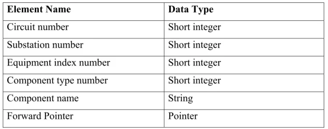
Because of these contained links and pointers, each component’s data object is known as a “trace” structure. Table 1 lists the elements in the trace component structure that are related to the reliability analysis module. Each trace structure contains 198 data elements, including pointers to other structures.

Table 6.1 DEW Component Trace Structure Element

Element Name Data Type

Circuit number Short integer

Substation number Short integer

Equipment index number Short integer Component type number Short integer

Backward Pointer Pointer

Feeder Path Pointer Pointer

Brother Pointer Pointer

//…Elements added for reliability analysis module

Segment Pointer Pointer

Forward Segment Pointer Pointer Backward Segment Pointer Pointer Feeder Path Segment Pointer Pointer

. . . . . .

Due to the large size of the trace structure, only the elements which are employed by the reliability analysis module are listed in Table 1. Several segment trace pointers are included in the structure. The Segment Pointer is used to find the primary sectionalizing device for a component. Sectionalizing devices in a circuit are linked in a doubly linked list via the Forward Segment Pointer and the Backward Segment Pointer. Sectionalizing devices are also linked with the Feeder Path Segment Pointer, which is similar to the Feeder path pointer for components, except that only sectionalizing devices are processed.

discussed previously. Circuit traces represent the order in which an algorithm processes the components of the system. As indicated earlier, a circuit analysis program must efficiently manage large quantities of system and equipment data. The pointers and linked lists compact the data storage and reduce algorithm execution time.

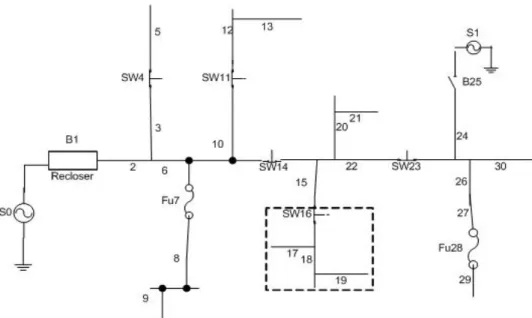
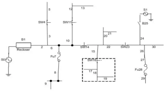
Here we provide an overview of using circuit traces. Figure 6.1 is an example circuit used to illustrate the application of circuit traces. Source S0 is the original source of the circuit of interest, and S1 is the alternate source. S1 is separated from the circuit of interest by the open switch SW25.

traces. These traces along with the notation used to indicate the trace, are defined as follows:

FTm = forward component trace beginning with component m (if m is not specified, FT begins from the substation). FT in the example circuit is given by

FT= B1 Æ 2 Æ 3 Æ SW4 Æ 5 Æ 6…… (6.1) BTm= backward component trace beginning with m; as illustrated by

BT15 = 15 Æ SW14 Æ 13 Æ 12 Æ SW11 Æ 10 Æ 9…… (6.2) FPTm = component m’s feeder path component trace, as illustrated by

FPT15 = 15 Æ SW14 Æ 6 Æ 2 Æ B1. (6.3) ECT = ending component trace, here for the example circuit is given by

ECT=5 Æ 9 Æ 13 Æ 17 Æ 18 Æ 19…… (6.4) The circuit traces discussed above are basic circuit traces. For reliability analysis, it is more efficient to work with pointers to segments and to perform traces based on these pointers. The segment circuit traces used in this research are as follows:

FSTm = forward segment trace from segment m, (if m is not specified, the forward trace will begin with the substation). In the example circuit, FST is given by

FST= B1 ÆSW4 Æ Fu7 Æ SW14 …… (6.5) FPSTm = feeder path segment trace (It is performed relative to a given

segment m). For instance, if we trace from the segment of interest, segment SW16, FPSTSW16 is given by

FPSTSW16 = SW16 Æ SW14 Æ B1. (6.6) AFT = alternative feed trace. In the example circuit, there is only one

alternative source, so AFT is given by

AFT = SW25 (6.7)

If there is more than one alternative feed for the circuit, then AFT would consist of the linked list of all alternative feeds.

7. Computer Algorithm 7.1 Introduction

This chapter presents the computer algorithm used to develop the reliability analysis (RA) sets. The algorithm is implemented with linked lists. A notation in terms of linked lists is introduced to describe the algorithm. A software design for implementing the algorithm is also discussed. Along with the presentation of the algorithm, the example circuit illustrated in Figure 6.1, is used to explain the development of the RA sets.

7.2 Algorithm

In what follows, we assume for the example circuit that the segment of interest is given by

{S} = {SW16} (7.1) We first conduct a forward component trace (FCT), beginning with the substation, so that we can determine the SW set and set up segment pointers. This can be expressed as

FCT Î SW, pFSeg, pBSeg, pSeg (7.2) where

pFSeg = pointer to forward segment (in the example circuit, segment B1’s pFSeg pointer is pointed to segment SW14)

pSeg = pointer to segment device for component (In the example circuit, all the components in segment SW16, components 17, 18 and 19, have their pSeg pointed to SW16)

The expression (7.2) is read as the Forward Component Trace (FCT) yields the SW set and sets the pointers pFSeg, pBSeg, and pSeg. Note that the notation used here is always to have pointers begin with a small ‘p’.

For the example circuit,

SW = {B1, SW4, Fu7, SW11, SW14, SW16, SW23, Fu26, SW25} (7.3) In the FCT, we can also find the ending components that make up the EC set, by using the following condition

If a component’s forward pointer points to its brother pointer[6], then this component is an ending component.

Thus,

FCT Î EC (7.4)

There is a set of pointers representing the list of existing alternate feeds, AF, which can be set up during the FCT as well. If a component’s adjacent component, say component A, belongs to another circuit and is fed by another substation, it means the original circuit is connected to an

be traced via a FPST. In this way, we can collect all the available alternate sources. Thus

FCT Î AF (7.5)

Note that for each segment stored in the AF set, there are two ending components. One corresponds to a component in the EC set, and the other component exists in the adjacent circuit.

Since IS consists of all the sectionalizing devices in the feeder path of S, we can use a FPSTs to obtain the IS set, as well as the PD (protective device) set, as given by

FPSTs ÎIS, PD (7.6) For the segment of interest S in the example circuit

IS= {SW16, SW14, B1} (7.7)

PD = {B1} (7.8)

The logic used to develop the L set is as follows:

• Perform a FST. When the FST encounters a segment whose primary protective device belongs to the PD set, this segment is in the L set. • Otherwise, when the FST encounters a segment whose primary

Thus,

FST Î L (7.9)

Following the steps described above, we obtain the L set for the segment of interest S

L= {B1, SW4, SW11, SW14, SW16, SW23} (7.10) The segments in the SSL set may be isolated from S and the original source, so that the power can be restored from the original source. SSL is given by the following set operations

SSL=L ∩ NIS (7.11)

where NIS= SW – IS.

Applying Equation (7.11) in the example circuit, and using expressions (7.3), (7.7) and (7.10), we obtain

SSL= {SW4, SW11, SW23} (7.12) The NSL set has only one element – the segment of interest S. All the failed components in the segment of interest must be completely repaired before power can be restored to S.

The segments in the SL set can be switched away from the segment of interest S, so that if the failure occurs in the SL set, S may be fed from an alternative source. The SL set is given by the following set operation

SL= L ∩ IS – {S} (7.12)

In the example circuit, applying expressions (7.1), (7.7) and (7.10), we obtain

SL= {B1, SW14} (7.13) If the failed component lies in the SAF set, it is possible to restore power to S when system constraints are not violated. The system constraints that are of interest here are the power handling capabilities of the equipment. Of particular interest is the remaining power handling capability of each piece of equipment. In order to find the SAF set, we conduct feeder path segment traces both from an alternate source and the segment of interest S, FPSTAF and FPSTS, respectively. When these traces encounter a common path, then the SAF set is not empty. The SAF set includes the segments in the common path except the first segment that the feeder path traces meet in the common path. Thus,

In the example circuit,

SAF= {B1} (7.15)

The NSAF set includes all the segments for which it is not possible to restore power to S from an alternative source. All the failed components in these segments must be completely repaired before restoring power to S. The NSAF set is given by set operation:

NASF = SL – SAF (7.16)

In the example circuit, using expression (7.13) and (7.15), we get

NSAF= {SW14} (7.17)

The segments in the SF set may be isolated from S and an alternative source, so that power can be restored to S from the alternative source without violating system constraints.

The NSF set includes all the segments which may be isolated from S and an alternative source, but for which it is not possible to restore power to S because of system constraint violations. All the failed components in these segments must be completely repaired before power can be restored to S.

from the alternative feed (AF). If there is more than one alternative feed in the system, the minimum capacities encountered in the feeder path component traces FPTAF for all the available sources in the AF set must be compared. For instance, there are n alternative feeds in the system. Let

CAFk = minimum remaining component power capacity in the FPTAF for the

kth alternative feed, k =1, 2, 3 …n (7.18)

CAFm =

max

Thus CAFm represents the greatest minimum remaining capacity available among the alternative sources. For example, as demonstrated in Figure 7.1, there are two alternative sources, AF1 and AF2. The segment of interest is marked as S. As indicated in the figure, the power required by S is 5 KW. The numbers on the alternative feed components stand for the remaining capacity (units of KW) of the components.

According to Equation (7.18) and (7.19),

CAF1= min {10, 5, 30} = 5 CAF2 min {40, 20, 20, 10} = 10 CAFm = max { CAF11 , CAF21}

=max {5, 10}

=10

So

AFm = AF2 (7.20)

Even though the minimum remaining capacity on the feeder path from AF1 is equal to the required power in S, pulling the power from AF1 to S will fully utilize component AF12. Thus AF2 is chosen since it has more remaining capacity on the feeder path.

In the general case, the segment of interest is not directly connected to the alternative feeds as shown in Figure 9. So FPT traces in the circuit of interest are also required to determine remaining power handling capabilities. In essence, component traces from the segment of interest to all alternative sources are required to check power handling capacities.

In summary, the Circuit traces which yield the reliability analysis (RA) sets are shown in Table 7.1

Table 7.1 Summary of Traces Used to Develop the RA Sets Algorithm Steps Traces in the Circuit Model

Step 1 FCT Î SW, pFSeg, pBSeg, pSeg, EC, AF

Step 2 FPSTs Î IS, PD

Step 3 FST Î L

Step 4 FPSTAF, FPSTS Î SAF

Step 5 FPTAF Î SF or NSF

7.3 Power Flow Calculation

In order to get the required power or remaining capacity of a component, the power flow needs to be calculated. The Power Flow

algorithm is based on the two-port element model and the tree traverse [8]. It is carried out by several iterations. Every iteration consists of a backward traverse, followed by a forward traverse of all the elements. The backward traverse calculates the currents through all the elements. The forward

traverse will calculate the voltage drops across elements. These calculations are represented by the following equations.

(7.21) j j i j V I Z V = − (7.22) * * j load m j V S I I =

∑

where

Ij= current through element j

Im= current through directly connected downstream element fed by

elements j

Sload = load attached to element j

Vj = voltage at downstream port of element j

Vi = voltage at upstream port of element j

Zj= the impedance of element j.

The sequential algorithm for the Radial Power Flow is given as follows: 1. Starting from an ending element, backward traverse the tree

element-by-element. Equation (7.21) is applied to calculate the current for each element.

2. Starting from the source or root element, forward traverse the tree element-by element. Equation (7.22) is applied to

calculate voltages for each element.

3. Check the convergence criteria. If converged, stop; otherwise, go back to Step 1.

Once the power flow calculation is completed, then

FPTAF Î SF or NSF (7.23) In the example circuit, assuming system constraints are not violated,

7.4 Software Design

Figure 7.2 shows a sequence diagram which describes a software implementation of the reliability analysis algorithm. It illustrates the interactions among the objects and packages involved in the calculations. Two objects, RA of type Reliability Analysis, and PF of type Power Flow Analysis, and four packages- Circuit Model, RA Sets, Indices Calculation, and Reliability Data- are illustrated in the sequence diagram. This diagram visualizes the dynamic aspects of the reliability analysis software application.

As shown in Figure 7.2, after the user selects the segment of interest with the message Pick _Seg( ), the Reliability Analysis object sends the FCT() message repeatedly (as indicated by * ) to the Circuit Model package, corresponding to Step 1 in Table 7.1. Note that messages are named after the traces that are performed. Signatures of messages shown in Figure 7.2 are defined in Table 7.2. In essence, FCT( ) provides a specialized iterator that implements the Forward Component Trace. The FCT( ) message called repeatedly, returns component pointers in the order of the FCT trace. Please refer to Table 7.1 for the details of the component structure. Reliability Analysis uses the returned components to set up segment pointers and the sets SW, EC and AF.

Table 7.2 Summary of Messages in the RA Sequence Diagram

Reliability Analysis sends the message FPST(S) (S is the segment of interest passed in as a parameter) repeatedly to the Circuit Model, corresponding to Step 2 in Table 7.1. Circuit Model traces through the whole circuit and returns segment pointers in the order encountered in the FPST, and these segments are used to set up the PD set and IS set.

Messages Return Value

FCT ( ) Component pointer

FPST ( ) Component pointer FST ( ) Component pointer

Min_Cap ( ) Double representing the minimum remaining power capacity of the components on the alternative feed feeder path

Max_Cap( ) Double representing the maximum of the minimum remaining capacities available among all the

alternative feeds

GetCus ( ) Integer representing the number of customers attached to a component

setOperation_Org( ) RA sets for the original circuit setOperation_AF( ) RA sets for the alternative source. Get_Sets( ) Arrays of component pointers

Get Data ( ) Array of doubles representing annual failure rate, repair time for a component and switch operation time

Corresponding to Step 3 in the Table 7.1, the message FST( ) is sent repeatedly to the Circuit Model to set up the L set. Then set operations are performed to derive the sets NIS, SSL, NSSL, SL, and NSL. The development of these sets depends only on the original circuit, regardless of whether alternative sources are available or not.

If there are alternative feeds, via the message FPST (AF), the Circuit Model can achieve the matched components for reliability analysis to set up the SAF set. This is the fourth step shown in Table 7.1. Once the SAF set is available, the power flow calculation is called to check the system constraints. The Message Min_Cap( ) is sent repeatedly to the circuit of interest and all alternative feed circuits. In order to determine the remaining power handling capability, PF sends the message FPT(AF) to conduct the feeder path traces from all the alternative feeds. Then applying Equation (7.19), the maximum remaining capacity is obtained. The SF set and NSF set now be determined.

Then the message SetOperation_AF( ) is used to determine the rest of the reliability analysis sets. Once all the sets of Figure 5.2 are determined and the number of customers in each segment is obtained, reliability indices can be calculated. The computation of reliability indices will be described in the next chapter.

8. Reliability Indices

This analysis relies on two general classes of information to estimate the reliability: component reliability parameters and system structure. Using system structure and component performance data, we can evaluate the reliability of specific load points or the whole distribution system. The structure information is achieved by the circuit traces presented previously. In the following paragraphs the performance data is discussed.

Predictive reliability techniques suffer from data collection difficulties. Simplifying assumptions (default values) are required for practical analysis of distribution systems.

8.1. Functional characterization

The availability of component functionally is characterized by the following indices:

• Annual Failure Rate = the annual average frequency of failure • Annual Down Time = the annual outage duration experienced

at a load point.

The failure rate for segment i, FR_i, is the sum of the failure rates of all the components contained in the segment i as given by

∑

n = the number of components in segment i.

The average repair time for a segment i, REP_i, can be calculated by

∑

∑

Frj = the failure rate for component j

Repj = the average repair time for component j n = the number of components in segment i.

These indices are computed for each segment in the feeder. All load points within a segment experience the same failure rate and down time.

In the reliability analysis program, failure rates and repair times from field data are preferred. When this data is not available, default values are fetched from a table in the relational database which has generic average failure rates and repair times for each type of device.

8.2. Reliability Indices Calculation

After finding the reliability analysis sets for the segment of interest S, we can calculate the reliability indices. First assume there is a single failure incident.

The down time for the segment S, DT_S, is given by i SFSSL i i i NSF NSAFNSL i i S FR REP FR SOT DT =

∑

∑

SOTi = switch operation time to re-supply segment S due to the failure of

segment i.

Note that the reliability analysis algorithm presented here assumes that switch operations can always be performed faster than repairs.

The customer average interruption duration index (CAIDI) for a segment is the same as DTs

CAIDI = DTs (8.4) Once the down time for each segment is calculated, and given the number of customers attached to each segment, the total customer down time, DTC, for a given circuit can be calculated by

i circuit i i C DT DTC =

∑

Since the failure rate and down time is known at each segment on the feeder, the system index SAIDI (system average interruption duration index) is then given by

∑

The average restoration time for segment Sis computed as

∑

8.3. Relative Reliability Index

A new measure of reliability referred to as ‘Relative_CAIDI’ is introduced here. Relative_CAIDIj helps to identify the areas that need improvement. Relative_CAIDIj is given by

j

_

CAIDI

CAIDI

CAIDI

Relative

=

CAIDIckt= average CAIDI for the circuit of interest

Thus

• If Relative_CAIDIj = 1, then the customers in segment j have average reliability

• If Relative_CAIDIj < 1, then the reliability of the customers in segment j is less than average

• If Relative_CAIDIj > 1, then customers in segment j have reliability better than average.

Figure 8.1 Example Circuit for Relative_CAIDI

In Figure 8.1, the number attached to each sectionalizing device is the

Relative_CAIDIj for that segment. We can see segments such as P11, P12, P2, P31, and P4, have reliabilities greater than the average level of Circuit

C1, while segments such as P52, P71, P72, P63, have reliabilities poorer than the average value.

9. Distributed Generator Placement

In the evolving energy industry, emerging distributed generator technologies have the potential to provide attractive, practical, and economical generation options for energy companies and their customers. Distributed resource technologies range in size from 3-10 kW for residential systems to 50-500 kW for commercial users to 1-50 MW in the industrial market segment. Primary opportunities lie in using these technologies to

(1) improve the service and delivery of energy to end users (2) support the operation and management of transmission and distribution systems.

This work does not consider the islanding of distributed generators (that is the generator operating without substation supply).

A distributed generator is often placed at a substation because no further land purchases are needed. However, locating generators at substations, distributed generator acts only as a back up power source, which may not contribute significant reliability improvement as far as the entire system is concerned. Instead, generators located further out on a circuit can often significantly affect system reliability. It is necessary to evaluate the effects of different placements of distributed generators. In case studies in the next chapter we will see that locating the DG at the end of the circuit produces more reliability improvement than placing it at the substation.

10. Case Studies 10.1 Introduction

Reliability is affected by the following • Varying loading

• Switch/protective device placement • Switch operation times

• Available alternative feeds • Equipment current limits • Equipment failure rates • Equipment repair times.

The following examples will illustrate the effect of some of these variations. In this chapter the improvement of reliability by distributed generators is demonstrated through three case studies. The first case study uses a test circuit developed to show the influence of various factors on system reliability. The second case study tests the reliability analysis program on a large scale system. It also shows how different DG placements affect the reliability of the system. The third example demonstrates how reliability changes with system load variation.

10.2. Case Study One

System 1 is presented in Figure 10.1. This is a system with only one substation Sub1, and 31 customers. The number attached to each

Figure 10.1 System 1 for Case Study One

Line Lp611 is assumed failed and switch p61 is assumed to have opened. Thus the set of segments losing power due to the operation of p61 is

{p71, p72, p8, p62, p63}

Assume that segment p62 is the segment of highest priority. Applying set Equations (1) - (8) relative to segment p62 gives

L= {p11, p12, p31, p61, p62}

Lp611

NSSL= {p11, p12, p61, p62} NSL= {p62}

SL= {NULL}

and SF= NSF= NSAF= {NULL}

Using the default failure rate and repair time in Table 10.1, we can calculate the annual down time for segment p62 as 0.355 hours. Since there are no alternate feeds in the system, only the failure occurring in the SSL set, which is p31 in this example, can be switched away; for the failure in the rest of Set L, segment p62 has to experience the restoration time for the failing component being completely repaired.

Table 10.1 Equipment Index Table

Equipment

Index Component Type Default Failure Rate

Default Repair Time (Hrs/Yr)

0 Substation 0.1 5

1 Disconnect switch 0.001 5

2 Load break switch 0.001 5

3 Supervisory switch 0.001 5

4 Cutout Switch 0.001 5

8 Remotely set recloser 0.001 5

9 Sectionalizer 0.001 5

10 Breaker 0.001 5

11 Network protector 0.001 5

13 Remotely set relay 0 5

14 Reclosing device 0.001 5

15 Fixed tap transformer 0.01 5

16 Distribution transformer 0.01 5

17 Network transformer 0.01 5

18 Regulating transformer 0.01 5

19 Voltage regulator 0.01 5

20 Fixed shunt capacitor bank 0.01 5

21 Switched shunt capacitor bank 0.01 5

33 3-Phase line 0.01 5 34 2-Phase line 0.01 5 35 1-phase line 0.01 5 37 3-Phase cable 0.01 5 38 2-Phase cable 0.01 5 39 1-Phase cable 0.01 5

41 3-phase underground cable 0.01 5

42 2-Phase underground cable 0.01 5

43 1-Phase underground cable 0.01 5

44 Arrester 0.001 5 45 Current transformer 0 5 46 Potential transformer 0 5 47 Communication transmitter 0 5 48 Communication receiver 0 5 49 Combination switch 0.001 5

52 Ground relay 0 5

53 Phase Imbalance Relay 0 5

54 Elbow Switch 0.001 5

56 Cable, Station Pole 0.001 5

59 Normally Open Point Location 0 5

60 Pole Top Switch 0.001 5

In Figure 10.2, an adjacent circuit C2 is added to the system. This circuit has some remaining capacity, which means it is possible for it to supply some power to circuit C1.

L68

31

Again, applying the set equations we get L= {p11, p12, p31, p61, p62} SSL= {p31} NSSL= {p11, p12, p61, p62} NSL= {p62} SL= {p11, p12, p61} SAF= {P11, p12, p61} NSAF= {NULL} SF= {p11, p12, p61} NSF= {NULL}

If the failure happens in the set SAF, p62 can be restored from circuit C2 without violating system constraints, because Sub2 has plenty of capacity to support its adjacent circuit. The set NSF is empty, so SF=SAF.

The significant drop comes from power being restored from Sub2, and p62 does not need to wait for the failing component to be completely repaired. In this case, the down time will be the switch operation time instead of the repair time for the failing component. The alternate source also improves the reliability of the entire system. Table 10.2 shows a comparison of reliability indices for System 1 and System 2.

Table 10.2 Improvement of Reliability

Reliability Indices System1 without Alternate Feed System 2 with Alternate Feed Percent Improvement SAIDI(Hrs/yr) 0.002 0.001 50% CAIDI(Hrs/yr) 0.305 0.176 42%

If the load on circuit C2 becomes heavier, substation Sub2 might lose the capacity to pick up the load on C1. For example, when we lengthen line L68 or add 5600kw load to it, pushing the load near to the overload point for the line, the annual down time for segment p62 will jump back to 0.355 Hrs/yr, and the system CAIDI will also go back to 0.305 Hrs/yr. It means the load point of interest cannot be restored from the alternate source because system constraints will be violated. Now we can see how the availability of alternate feeds and the change of the system loading impact the system reliability. Next we will illustrate how a distributed generator enhances the reliability of the system. As it is illustrated in Figure 10.3, a distributed generator DR0 is

Figure 10.3 System 3 for Case Study One: Adding a Distributed Generator

When the load in circuit C2 grows so that substation Sub2 can no longer pick up any load in circuit C1, the distributed generator DR0 will be activated. This provides a source of power that can also be used to supply loads switched from C1 to C2. The reliability of circuit C1 will increase due to the availability of DR0. Table 10.3 shows the improvement in annual down time for the segments in circuit C1.

31

9

Table 10.3 Comparison of Reliability Improvements

Down Time (Hrs/yr) Segment Name

Without DR0 With DR0 Improvement

p63 0.405 0.095 77% p62 0.355 0.085 76% p61 0.31 0.13 58% p71 0.36 0.18 50% p72 0.41 0.23 44% p12 0.22 0.13 41% p8 0.46 0.28 39% p31 0.265 0.175 34% p4 0.27 0.18 33% p2 0.27 0.18 33% p51 0.28 0.19 32% p52 0.37 0.28 24% p32 0.465 0.375 19% P11 0.13 0.13 0%

From Table 10.3, we notice that the segments close to DR0 (etc. P62, P63) have more improvement than those (etc. P52, P32) far from DR0. The segment P11, which is next to source Sub1, has no improvement at all. This is because as the distance between the segment of interest and the alternative feed increases, the alternative source needs to supply more and more power to its adjacent circuit in order to restore the segment of interest, and its

availability of DR0 will not make any additional contribution to the reliability of its adjacent circuit.

10.3. Case Study Two

Figure 10.4 illustrates a large scale system. It has two circuits consisting of 5,421 components. The overall system contains 222 segments. Using the RA program, it takes about half of a second to calculate the system reliability indices on a personal computer (Pentium 4 CUP 2.40GHz,

512MB of RAM). A reliability analysis report for the system shown in Figure 10.4 is shown in Appendix A.

Figure 10.5 is part of the system shown in Figure 10.4. A small circuit C3 fed by substation Sub2 is added to the original system in Figure 10.5.

Figure 10.5 Addition of Substation and DG to System Shown in Figure 10.4

A DG is placed next to Sub2, which has the same effect as putting it in the substation, because there is not any load between Sub2 and the DG. Line L_C1 is the component that exists in the original system (prior to the addition of Sub2 and C3) and is very close to Circuit C3.

When circuit C3 is heavily loaded, C3 is not able to supply any power to its adjacent circuit. Under this condition, the down time for line L_C1 in

L_C32 L_C1 L_C31 DG Sub 2 C3

locating the DG in Sub2 does not improve the reliability of L_C1 at all. From Case Study One, we can predict that placing the DG in Sub2 will not increase the reliability of the rest of the original system either (the segments further away from the adjacent circuit have less improvement).

Figure 10.6 DG at the End of Circuit

If the DG is placed at the end of circuit C3 connecting to L_C32, as shown in Figure 10.6, the down time for line L_C1 drops to 0.360 Hr/Yr. This significant change in the reliability of L_C1 is due to the change of the DG’s placement. When the DG is located in Sub2, C3 dose not have enough remaining capacity to support its adjacent circuit. Placing the DG at the end of C3 provides capability to pick up the load on line L_C1 if the failure occurs in the original system. So the reliability of L_C1 dramatically

L_C32 L_C1 L_C31 DG Sub 2 C3

increases. Table 10.4 shows the system reliability improvement after adding the alternative source Sub2 and distributed generator DG.

Table 10.4 System Reliability Improvement for Case Study Two

System indices Without Alternate Feed

With Alternate

Feed and DG Improvement

SAIDI(Hrs/yr) 0.72 0.54 25%

CAIDI(Hrs/yr) 9.12 6.03 34%

10.4 Case Study Three

Previous reliability calculations have been performed for static load models and inherently make the assumption that system reliability is independent of load. In this case study, we investigate the reliability improvement over a time varying load curve.

Figure 10.7 Circuit for Case Study Three

Figure 10.7 shows the same part of the circuit that we studied in Case Two. Now we look into the load curve of line L_C32 for a weekday in January. As illustrated in Figure 10.8, the estimated load of L_C32 fluctuates during the 24-hour period, and reaches its peak value around 6pm to 7pm, when most of people return home and turn on their electric utilities.

L_C32

L_C1 Sub 2

Estimated Load Down Time

Figure 10.8 Down Time Variation with Varying Load of L_C32

Along with time, the variation of the reliability of line L_C1, which is reflected by its down time, is also shown in Figure 10.8. We can see that from 12am to 4pm, when the load in line L_C32 remains relatively low, the down time for line L_C1 stabilizes at 0.36Hr/Yr. When the load of line L_C32 rapidly grows in the evening, it triggers a dramatic increase in the down time, which jumps from 0.36Hr/Yr to 0.805Hr/Yr. After that summit period, from 6pm to 9pm, the down time of line L_C1 decreases to 0.36Hr/Yr again. This change of the reliability of line L_C1 with the variation of load in line L_C32 is because the reliability depends on the

0.1 0.2 0.3 0.4 0.5 0.6 0.7 0.8 Down Time (Hr/ yr )

goes up to the point close to being over loaded, it has no remaining capability to support the original circuit any more. From the reliability analysis sets explained in Chapter 5, set SAF is empty in this case. If any failure occurs in the circuit except in set SSL, the load point of interest (here it is L_C1) will experience the interruption for the entire repair time of the failure point. This is why it annual down time significantly increases.

If the time varying load on line L_C32 is reduced such that its peak dose not exceed 4000KW, as illustrated in Figure 10.9. In this case the reliability of line L_C1 remains at a high level throughout the load cycle, which is indicated by the constant down time 0.36Hr/Yr.

0 0.1 0.2 0.3 0.4 Do w n Time (H r/Yr )

11. Conclusions and Further Research 11.1. Conclusions

In this work, we have presented a reliability analysis algorithm. Set calculations coupled with circuit traces are used to calculate the reliability of a given load point and an entire system. An application has been developed to implement this algorithm. The placement of distributed generation and its effects on reliability is investigated. An evaluation of reliability over time varying load curves is also presented. Three case studies are demonstrated, where reliability indices produced by the reliability analysis program for particular segments and the entire system provide concrete figures to assess reliability improvements.

Conclusions from the investigations are:

• The created reliability analysis algorithm is fast enough on large systems to be used in interactive design studies

• A new reliability index, Relative_CAIDI, has been proposed which makes it easier for a design engineer to find circuit locations in need of improvement

• Placing distributed generators further out on a circuit, instead of locating them in the substation, can help enhance a system’s reliability • It is practical to estimate reliability as a function of time (loading).

11.2. Further Research

Besides adding a distributed generator, there are also other ways to enhance a system’s reliability. For example, we can change the system structure by adding more protective devices or by moving sectionalizing devices forward or backward. And then if we recalculate the reliability indices for the entire system, and compare them with the original values, we can see whether the change improves the reliability or not.

We have proposed a new reliability index, Relative_CAIDI. If the Relative_CAIDI for a given load point is less than 1, it means the reliability of the affected customers is less than average. Further research could focus on automated system structure modifications which are base upon the value of Relative_CAIDI.