https://doi.org/10.1007/s11263-018-1121-3
Deep Sign: Enabling Robust Statistical Continuous Sign Language
Recognition via Hybrid CNN-HMMs
Oscar Koller1 ·Sepehr Zargaran1·Hermann Ney1·Richard Bowden2 Received: 1 February 2017 / Accepted: 3 September 2018 / Published online: 5 October 2018 © The Author(s) 2018
Abstract
This manuscript introduces the end-to-end embedding of a CNN into a HMM, while interpreting the outputs of the CNN in a Bayesian framework. The hybrid CNN-HMM combines the strong discriminative abilities of CNNs with the sequence modelling capabilities of HMMs. Most current approaches in the field of gesture and sign language recognition disregard the necessity of dealing with sequence data both for training and evaluation. With our presented end-to-end embedding we are able to improve over the state-of-the-art on three challenging benchmark continuous sign language recognition tasks by between 15 and 38% relative reduction in word error rate and up to 20% absolute. We analyse the effect of the CNN structure, network pretraining and number of hidden states. We compare the hybrid modelling to a tandem approach and evaluate the gain of model combination.
Keywords Sign language recognition·Hybrid approach·CNN-HMM·Statistical approach·Sequence modelling
1 Introduction
Face-to-face communication is often the preferred choice, when either important matters need to be discussed or informal links between individuals are established. Ges-ture is a key part in such human-to-human communication. It helps us to better understand the other party. However, the role of visual cues in spoken language is not well defined. As such, the task of gesture recognition is also not accurately defined. This renders comparison of algo-rithms and approaches difficult. Sign language on the other hand provides a clear framework with a defined inventory and grammatical rules that govern joint expression by hand (movement, shape, orientation, place of articulation) and by face (eye gaze, eye brows, mouth, head orientation). This makes sign languages, the natural languages of the deaf, a perfect test bed for computer vision and human Communicated by Edwin Hancock, Richard Wilson, Will Smith, Adrian Bors and Nick Pears.
B
Oscar Koller1 Human Language Technology and Pattern Recognition,
RWTH Aachen University, Aachen, Germany
2 Centre for Vision Speech and Signal Processing, University
of Surrey, Guildford, UK
language modelling algorithms targeting human computer interaction and gesture recognition. The rules governing the interaction of hands and body, referred to as the manual and non-manual parts—are well defined by sign language theory. Videos represent a time series of dynamic images and the recognition of sign language therefore needs to be able to cope with variable input sequences and execution speed. Different schemes are followed to achieve this ranging from sliding window approaches (Ong et al.2014) to tem-poral normalisations (Molchanov et al. 2015) or dynamic time warping (Krishnan and Sarkar 2015). While the field of automatic speech recognition is dominated by Hidden-Markov-Models (HMMs), they remain rather unpopular in computer vision related tasks. For instance CVPR, by many regarded as the top conference of computer vision, had only three out of a total of over 700 submissions in the year 2017 that were using HMMs (Koller et al. 2017; Richard et al.2017; Schober et al.2017). This may be related to the comparatively poor image modelling capabilities of Gaus-sian Mixture Models (GMMs), which had been traditionally used to model the observation probabilities within such a framework. More recently, deep Convolutional Neural Net-works (CNNs) have outperformed other approaches in all computer vision tasks. In this work, we focus on integrating CNNs in a HMM framework, extending an interesting line
of work (Koller et al.2015b,2016a; Le et al.2015; Wu and Shao2014), which we will discuss more closely in Sect.2.
This manuscript presents the extended version of our pre-vious work (Koller et al.2016b), where we first presented a powerful embedding of a deep CNN in a HMM framework in the context of sign language and gesture recognition, while treating the outputs of the CNN as true Bayesian posteriors and training the system as a hybrid CNN-HMM in an end-to-end fashion. With this method we are able to achieve a large relative improvement of over 15% compared to the state-of-the-art on three challenging standard benchmark continuous sign language recognition data sets. In the scope of this extended manuscript, we make several additional contribu-tions and have completely reran all experimental evaluation to allow us to provide more extensive results and deeper insights:
1. We significantly add to the theoretical explanation of the hybrid approach, with the aim of making its idea more accessible to newcomers to the field.
2. We analyse the effect of both CNN- and HMM-structure on the hybrid approach.
3. We investigate the effect of using out-of-domain data to train the network prior to finetuning using in-domain data.
4. We show that different training iterations provide com-plementary classifiers, which are able to further boost recognition when employed as ensembles of hybrid CNN-HMMs.
The rest of this manuscript is organised as follows: Sect.2 discusses the related literature in depth. In Sect.3we intro-duce the theoretical basis of the presented hybrid approach. Differences w.r.t. the tandem approach are also described. The employed data sets are discussed in Sect.4. Section5 gives details on the implementation in order to ensure repro-ducibility, which is followed by the actual experimental evaluation in Sect.6. Finally, we conclude the work in Sect.7.
2 Related Work
After the recent success of CNNs (LeCun et al.1998) in many computer vision fields, they have also shown large improve-ments in gesture and sign language recognition (Neverova et al.2014; Huang et al.2015; Koller et al. 2015b). How-ever, in most previous CNN-based approaches the temporal domain of video data is not elegantly taken into consid-eration. Most approaches simply use a sliding window or circumvent the sequence properties by evaluating the output in terms of per-frame overlap with the ground truth, e.g. in Pigou et al. (2018). Moreover, CNNs are usually trained on the frame-level. A few artificial data sets such as the
Mon-talbano gesture data set (Escalera et al.2014) provide frame labels. However, this is usually not the case, especially for sign language footage or other real-life data sets. Available annotation usually consists of sequences of signs without explicit frame-level information. As such, the focus of the field needs to move towards approaches that deal with vari-able length inputs and outputs that do not require explicit frame labelling. The difficulty in accurately labelling sin-gle frames for evaluation further supports the need for such change. Graphical models such as HMMs lend themselves well to tasks with inputs of variable length. As will be shown in this work, we are able to combine the best of different worlds when integrating HMMs and CNNs. A few works have joined neural networks and HMMs before in the scope of gesture and sign language recognition. Wu and Shao (2014) use 3D CNNs to model the observation probabili-ties in a HMM. However, they interpret the CNN outputs as likelihoods p(x|k)for an imagexand a given classk. Con-versely, Richard and Lippmann (1991) showed that neural network outputs are better interpreted as posterior probabil-ities p(k|x)in a Bayesian framework. In the field of speech recognition, Bayesian hybrid neural network HMMs were first proposed by Bourlard and Wellekens (1989) and became the approach of choice, particularly after the recent rise of deep learning. Le et al. (2015) followed this line of thought for gesture recognition, but only employed a shallow legacy neural network that was trained to distinguish twelve artificial actions. Koller et al. (2013,2014) achieved important results using GMM-HMMs for weakly supervised learning in the domain of sign language. However, hybrid models strongly outperformed the results (Koller et al. 2016a), which con-stituted first and preliminary work in this direction. CNNs were employed in a hybrid Bayesian framework to perform weakly supervised training with the purpose of learning hand shape classifiers that generalise across data sets. The main differences with respect to this manuscript are that we learn the CNN top down using nothing more than the anno-tated sign-words (which are modelled by a fixed number of hidden states), whereas Koller et al. (2016a) models signs bottom up with additional knowledge of the decomposition of sign-words into different hand shapes which form the build-ing blocks for signs. Moreover, in this work, we learn the CNN-HMM in an end-to-end fashion from video input to gloss output, whereas in the previous work, the intermediate hand shape-CNN serves as feature extractor for an additional GMM-HMM sign model (similar to the tandem approach introduced in Sect.3.3). In this so-called tandem modelling (refer to Sect.3.3), the GMM-HMM needs to be completely retrained, which adds significant computational overhead. In the proposed hybrid approach, no GMM-retraining is nec-essary and in the experimental evaluation of this manuscript we will show that our approach clearly outperforms Koller et al. (2016a). Wu et al. (2016) published a paper that is also
closely related to this work, but they do not interprete the CNN outputs in a Bayesian way, they use different inputs to the CNN (full body RGB and depth, as opposed to using a cropped hand patch) and different inputs to the HMM. Later, Granger and el Yacoubi (2017) provided a compari-son between a hybrid neural network HMMs and a recurrent neural network (RNN) on a gesture task, finding that both perform comparably, while the state-based representation of the HMM allows better insights in the internals of the model for potential error analysis. Recently, Connectionist Tempo-ral Classification (CTC) by Graves and Schmidhuber (2005) has received attention by the computer vision community in general (Assael et al.2016; Cui et al.2017; Rao et al.2017). CTC is a training criterion for recurrent neural networks and very related to HMMs. CTC has been shown to be a special case of the hybrid full-sum HMM alignment with a specific HMM architecture. As such CTCs are related to this work. However, we do not use recurrent or long short term mem-ory (LSTM) networks in this work. The interested reader may consult Bluche et al. (2015) for details on the comparison of CTC and HMMs.
Finally, this manuscript represents a more thorough ver-sion of Koller et al. (2016b), with much more extensive experiments. In addition, this manuscript analyses the effect of both CNN- and HMM-structure on the hybrid approach. It also investigates the effect of using out-of-domain data to pretrain the network prior to finetuning using in-domain data and the use of ensembles of CNN-HMMs in model combi-nation to further boost performance. Koller et al. (2017) even drop the dependence on a hand tracking system and take the re-alignment of hybrid models for sign recognition further.
Another related approach has been introduced by Bengio and Frasconi (1996), where a RNN is used to extract tempo-rally local information whereas a HMM integrates long-term constraints. The so-called input output HMM has been used by Marcel et al. (2000) in a basic gesture system that distin-guishes between two gesture classes, deictic and symbolic.
3 Continuous Sign Language Recognition
The problem to be solved is a sequence learning task, which means we want to predict a sequence of output symbolswN
1, in our case sign words (so-called “glosses”, representing
the semantics of the described word). Given an input video as a sequence of full images X1T = X1, . . . ,XT and the resulting preprocessed (e.g. tracked and mean-normalised) images x1T = x1, . . . ,xT, automatic continuous sign lan-guage recognition tries to find an unknown sequence of sign-words w1N for which x1T best fit the learned models. We assume that images and sign-words occur in an ordered fashion. It has to be noted that this requirement clearly dis-tinguishes the problem of sign language recognition from
the problem of translating from sign language to spoken lan-guage where re-orderings are necessary and monotonicity cannot be assumed.
3.1 Legacy GMM-HMM Approach
To find the best fitting sequence, we follow the statistical paradigm (Bahl et al.1983) using the maximum-a-posteriori simplification of Bayes’ decision rule, which has been suc-cessfully applied to Automatic Speech Recognition (ASR), hand writing recognition and statistical machine translation since the early 1970s. Given a loss function Lw1N,w˜1N between the true output sequencew1N and the hypothesised output sequence w˜1N, Bayes’ Decision Rule minimises the expected loss: x1T → wN 1 opt=argminw˜N 1 ⎧ ⎪ ⎨ ⎪ ⎩ wN 1 Pr wN 1|x1T ·LwN 1,w˜1N ⎫⎪⎬ ⎪ ⎭ (1) Often Bayes Decision Rule is simplified to the maximum-a-posteriori (MAP) rule, which is known to be equivalent for the case of the simple 0-1-loss.
x1T → wN 1 opt=argmax wN 1 Pr wN 1|x1T (2)
In sign language recognition the 0-1-loss corresponds to a minimisation of the expected sentence error rate, which counts an output sentence as wrong if a single recognised sign-word is wrong. However, for longer sentences, the sen-tence error rate does not correlate with the word error rate (WER) which is also known as edit distance and what we seek to minimise. As shown by Schlüter et al. (2012), the MAP rule is equivalent to the Bayes Rule for the WER as a loss function if max wN 1 Pr wN 1|x N 1 >0.5 (3)
Therefore, we follow the MAP rule as the optimisation criterion and maximise the class posterior probability dis-tribution Pr(w1N|x1T)over the whole utterance, as given in Eq. (2).
Decision theory allows us to split up the class pos-terior probability into the class prior Pr(w1N) and the class-conditional probability Pr(x1T|w1N), which can then be modelled by different information sources. The first term can be interpreted as word sequence knowledge which can be approximated by a n-gram language model estimating
p(w1N). The second term represents the actual visual knowl-edge, which historically used to be modelled by generative GMMs.
wN 1 opt=argmaxwN 1 p wN 1 · p x1T|w1N (4)
Expressing the class-conditional probability in terms of a HMM adds the hidden variables1T:
p x1T|w1N = s1T p x1T,s1T|w1N (5) = sT 1 T t=1 p xt,st|x1t−1,s1t−1, w1N (6) = sT 1 T t=1 p xt|xt1−1,s1t, w1N ·p st|x1t−1,s1t−1, w1N (7) = s1T T t=1 p xt|st, w1N ·p st|st−1, w1N (8)
where the sum in Eq. (5) expresses all viable paths that lead to the same output sequencew1N. Equations (6) and (7) con-stitute reformulations with help of the chain rule. Assuming
sto be non-observable and a first order Markov process leads to Eq. (8). After applying the viterbi approximation, which considers only the most likely path and substituting every-thing into Eq. (4), we get:
wN 1 opt=argmaxwN 1 p wN 1 ·max sT 1 T t=1 p xt|,st, w1N · p st|st−1, w1N (9)
where in the legacy Gaussian mixture model (GMM)-hidden Markov model (HMM) approach for sign language recogni-tionpxt|,st, w1N
has typically been modelled as
p xt|,st, w1N = M m=1 cm·N (x, μm, Σ) (10) M m=1 cm =1 (11)
whereN (x, μ, Σ)is a multi-variate Gaussian with meanμ, covariance matrixΣandM is the number of mixture com-ponents (can differ between states of the same word). Legacy systems typically employed a globally pooled covariance matrixΣ to cope with the low amount of training samples per state and word. The expectation maximization (EM) algo-rithm is used to estimate the sufficient statistics of the GMMs. The number of EM iterations is usually optimised on held out data during the training phase of the system.
p(st|st−1, w1N)(referring to Eq. (9)) represents the state transition model, which is empirically known as part of the model having limited impact on the final result and can there-fore be pooled across all HMM states. In log-domain we often refer to it as the Time Distortion Penalties (TDPs). The depen-dency on the sequence of wordsw1Nmay be dropped, since the temporal sequence of statess1Tis defined to be a sequence of HMM states corresponding to a specific path through the word sequencew1N, which we implement as concatenation of automatons forw1N (using the word-to-state decomposition defined by the pronunciation lexicon and the word sequence annotations of the corpus).
3.2 Hybrid CNN-HMM Approach
Up to this point, we have deduced the standard HMM formula for recognition using a generative model for the emission probability. However, in the scope of the presented work we model the emission probability of the HMM p(xt|st, w1N)
by an embedded CNN, which is known to possess much more powerful image modelling capabilities than generative models such as GMMs. However, as pointed out by Richard and Lippmann (1991) and Bourlard and Morgan (1993), the CNN is a discriminative model whose outputs are estimates of the posterior probability and therefore cannot directly be inserted in the optimisation formula. Inspired by the hybrid approach known from ASR (Bourlard and Morgan 1993), we use Bayes’ rule to convert the posterior probability of the CNN to a likelihood. For easier understanding we intro-duce the sub-word labelα:=s, w1N, representing the state
sbelonging to the word sequencew1N. The CNN will hence be trained to model p(α|xt). We apply Bayesian inference, converting the posteriors to class-conditional likelihoods fol-lowing Bayes’ rule:
p(xt|α)= p(xt)·
p(α|xt)
p(α) (12)
where the prior probabilityp(α)can be approximated by the relative state label frequencies in the frame-state-alignment used to train the CNN.
For practical usage, we add several hyper-parameters to the implementation. These allow us to control the effect of the language model (γ) and the CNN label prior (β). Neglect-ing the constant frame prior p(xt), we finally optimise the following equation to find the best output sequence:
wN 1 opt =argmax w pw1Nγ·max sT 1 T t=1 p(α|xt) p(α)β ·p st|st−1, w1N (13)
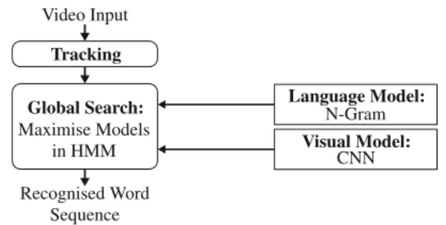
Fig. 1 Overview of the proposed CNN-HMM hybrid approach for con-tinuous sign language recognition
A general overview of the proposed hybrid CNN-HMM algorithm for recognition can be found in Fig.1. The hybrid approach has the positive property that during training only the CNN and the language model (LM) need to be retrained, while the HMM requires no training. For testing, the best hyper parameter values forγ,βand the pooled state transi-tion modelp(st|st−1, w1N)are found using a grid search.
Figure2summarises the resources we need to success-fully apply the hybrid approach: a dual corpus of sign videos (sentence-wise segmented) and corresponding sign-word annotations. In this work, we further employ the HMM frame-state-alignment coming from a HMM-GMM system as frame labelling, which can be replaced by an appropriate re-alignment scheme as shown in Koller et al. (2017).
3.3 Tandem Approach
An intermediate step between GMM-HMM and the hybrid CNN-HMM systems is the so-called tandem approach. It is very similar to the hybrid approach in the sense that it uses both a CNN and HMM. However, the CNN is not used as a classifier, but rather as a feature extractor. In the so-called tandem approach (Hermansky et al.2000) the activations of a fully connected layer or the feature maps of a convolu-tional layer are dumped, post-processed (Koller et al.2016a) and then modelled in a GMM-HMM framework. This cre-ates a significantly higher computational cost than the hybrid approach for extracting features and retraining a GMM sys-tem. Golik et al. (2013) found that in speech and handwriting
Fig. 2 Showing the employed resources (in light boxes on the left) to train the models for the hybrid CNN-HMM approach. The frame-state-alignment has been generated from the sign-word (gloss-) annotations using a GMM-HMM system from Koller et al. (2016a)
recognition the hybrid approach shows equal or superior per-formance compared to the tandem approach. We will verify this statement for sign language recognition in Sect.6.3. As discussed in Sect.2, in the gesture and sign language recog-nition literature to date, most other works either use the CNN outputs not in a Bayesian interpretation (Wu et al.2016) or employ the CNN as feature extractor comparable to the tan-dem approach. Figure 3shows the tandem and the hybrid approach side by side. We denote that the only difference is the visual model.
4 Data Sets
The experiments are carried out on three state-of-the-art continuous sign language data sets that have been used extensively to compare recent methods for continu-ous sign language recognition: RWTH-PHOENIX-Weather 2012, RWTH-PHOENIX-Weather 2014 and SIGNUM. Here, we provide an essential summary and some additional statis-tics on the word-class distributions. However, for further details on the data sets, the interested reader is directed to Koller et al. (2015a).
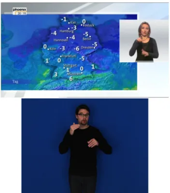
Single images of the corpora are depicted in Fig.4. Brief statistics on the three data sets can be found in Table1. Both RWTH-PHOENIX-Weather corpora (2012 and 2014) were first introduced by Forster et al. (2012) and Forster et al. (2014) and represent direct recordings of the broadcast news, being limited to the weather forecast domain. As such, the data can be regarded as challenging real-life footage cov-ering most difficulties you would expect from natural data (motion blur, transmission artifacts, fast signing, incomplete sentences, mis-signed words, interpretation errors, different clothing, etc.). RWTH-PHOENIX-Weather 2012 features a single signer interpreting the news into sign language, while RWTH-PHOENIX-Weather 2014 contains nine individuals covering varying amounts of the recorded programs.
SIGNUM was first introduced by von Agris et al. (2008b) and was recorded in a laboratory environment while carefully controlling the signing and recording conditions. However, deviations from word counts in Table1w.r.t. previous work are errata, while the underlying data has not changed. All data sets feature user-dependent setups as all individuals occur both in the training and in the test/development (dev) parti-tions. The RWTH-PHOENIX-Weather is freely available.1 It has to be noted that the actual annotation of PHOENIX 2014 and SIGNUM cover a larger variety of words than what the actual testing regime foresees. Therefore both data sets provide some mapping in order to join certain classes. This mainly arises due to the difficulty of the gloss annotation
1 It can be obtained at http://www-i6.informatik.rwth-aachen.de/
Fig. 3 Illustrating the difference between CNN-HMM tandem and hybrid approach. The former uses the CNN only as a feature extractor to train a subsequent GMM, while the later directly uses the CNN’s normalised posteriors probabilities for a labelαgiven inputx
Fig. 4 Example images showing the data sets employed in this work. RWTH-PHOENIX-Weather on the left and SIGNUM on the right
and manifests itself partly in inflected forms of the same words and in different words that are visually identical or very close. All referenced publications that report results on the data sets have been applying this simplification scheme, which is distributed with the data. The final number of classes that are distinguished in evaluation (see row ‘vocab-ulary’ in Table1) is 266, 1080 and 465 for PHOENIX 2012, PHOENIX 2014 and SIGNUM respectively. On SIGNUM the vocabulary is 10 words larger than the reported
vocabu-lary by the authors (von Agris et al.2008a). It is unclear what the cause for this is. Unfortunately the original authors can-not be reached anymore. The still frames in Table1refer to frames that have been automatically labelled as background during the HMM alignment.
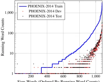
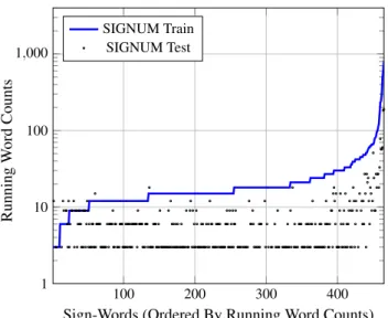
Figures5,6and7 show the distribution of word counts on PHOENIX 2012, PHOENIX 2014 and SIGNUM respec-tively. It can be seen that both PHOENIX 2012 and 2014 contain a large number of words with only a single occur-rence during training (so-called singletons), while SIGNUM statistics are different. On SIGNUM even the least frequent words occur at least 3 times, while most of them can be found at least 10 times in the training data. This is good for training and demonstrates SIGNUM’s artificial characteristic which (among other reasons) manifests itself in very low WERs.
5 Implementation Details
In this section, we describe the details to allow exact repro-ducibility of our experiments. Note, that we input single (still) frames to the CNN and the HMM covers the temporal mod-eling. Input frames are cropped hand images. The system has no explicit information on the location other than from the background of the cropped images.
5.1 Image Preprocessing
To track the right hand across all sequences of images we use a dynamic programming based approach (Dreuw et al.2006). In all data sets the right hand corresponds to the signer’s dominant hand, which is the hand that plays the principle role in signing. On the RWTH-PHOENIX-Weather corpora, we crop a rectangle of 92×132 pixel around the centre of the
Table 1 Key statistics of the
employed data sets PHOENIX 2012 PHOENIX 2014 SIGNUM
Train Test Train Dev Test Train Test
# Signers 1 1 9 9 9 1 1 Hours 0.51 0.07 8.88 0.84 0.99 3.86 1.06 Frames 46282 6751 799006 75186 89472 416620 114230 ∼Still frames – – 20% – – 38% – Running words 3309 487 65227 5540 6504 11127 2805 ∅Frames/word 14.0 – 9.8 – – 23.2 Vocabulary 266 – 1080 – – 465 – OOVs running – 8 – 28 35 – 9 OOVs [%] – 1.6 – 0.5 0.5 – 0.3
OOVOut-Of-Vocabulary, e.g. words that occur in test, but not in train. Dev refers to the development set
Fig. 5 Showing the distribution of words (and their counts) on the train and test partition of the RWTH-PHOENIX-Weather 2012 corpus. It can be seen that there are less than 100 sign-words occurring just a single time (singletons) imposing difficulties on the task
hand. The original images suffer a constant distortion due to the broadcast nature of the videos, which corresponds to a scaling of the image width by a factor of 0.7. To compensate for this distortion we enlarge the cropped rectangles to the square size of 256×256. On SIGNUM we directly crop a square patch of size 100×100 pixel and scale it up to 256×256. Thereafter the pixel-wise mean of all images in the training set is subtracted from each image. Finally, for data augmentation we follow an online cropping scheme, which randomly crop out a 224×224 (GoogLeNet) or a 227×227 pixel (LeNet and AlexNet) rectangle to match the size of images in our model which was pre-trained on ImageNet. The input to the CNNs consists of single cropped hand patches.
Fig. 6 Showing the distribution of words (and their counts) on the train, dev and test partition of the RWTH-PHOENIX-Weather 2014 corpus. It can be seen that there are more than 300 sign-words occurring just a single time (singletons) while few other classes occur more than 1000 times imposing difficulties on the task. Dev refers to the development set
5.2 Convolutional Neural Network Training
We base our CNN implementation on Jia et al. (2014), which uses the NVIDIA CUDA Deep Neural Network GPU-accelerated library. If not stated otherwise in the respective experiments, we opted for the GoogLeNet Szegedy et al. (2015) 22 layers deep CNN architecture with around 15 million parameters (for exact parameters refer to Table3). GoogLeNet has shown many times in the past, most notably in the ImageNet 2014 (ILSVRC) Challenge, that it can be quite effective in combining impressive performance with minimal computational resources. Much of the improve-ments in this architecture compared to others’ stems from the inception module which combines filters of different sizes after applying dimensionality reduction through a 1x1
Con-Fig. 7 Showing the distribution of words (and their counts) on the train, dev and test partition of the SIGNUM single signer corpus. In large contrast to the RWTH-PHOENIX-Weather corpora, it can be seen that hardly any sign-words occur just a single time (singletons). This shows the artificial nature of the data set and explains its comparative easiness
Fig. 8 Illustration of training scheme
volutional layer. The employed CNN architecture includes 3 classifying layers, meaning that besides the final classifier the network also includes two intermediary auxiliary clas-sifiers. Those encourage discrimination in earlier layers of the network. The loss of these auxiliary classifiers is added to the total loss with a weight of 0.3. All non-linearities are rectified linear units and each classifier layer is preceded by a dropout layer. We use a dropout rate of 0.7 for the auxiliary layers and 0.4 before the final classifier.
As mentioned in Sect.3, the CNN training scheme requires an initial frame-state-alignment. This originates from a GMM-HMM recognition system that is trained to re-aligning the frame-to-state mapping (frame-level alignment). This is illustrated in Fig.8. If not stated otherwise in the respective experiments, we use alignments from GMM-HMM systems reproducing the best published results on our chosen corpora.
For SIGNUM and RWTH-PHOENIX-Weather 2014 we use the best results published in Koller et al. (2016a) as align-ment, whereas for RWTH-PHOENIX-Weather 2012 we use Koller et al. (2015a). We split the frame-level alignment into a training (∼90% of the data) and a validation set (∼10% of the data) in order to be able to evaluate the per-frame accuracy of the CNN and stop the training when the vali-dation accuracy deteriorates. However, we noticed that this seldom happened and in these experiments we always chose the last training iteration. We first train the network on the ImageNet data set with 1.2 million high-resolution images in 1000 classes and then exchange the final classification lay-ers (on all three classifilay-ers) and finetune the network on the sign language data for 80,000 iterations with a mini-batch size of 32 images. We use stochastic gradient descent with an initial learning rate λ0 = 0.01 for CNN networks. We employ a polynomial scheme to decrease the learning rateλi for iterationias the training advances while reachingλi =0 for the maximum number of iterationsimax = 80k in our experiments for 4 epochs on PHOENIX (2012 and 2014) and SIGNUM. Only the experiment in Sect.6.4that analyses the effect of the HMM structure does not use the training and validation splitting. Instead it uses all available training data for training the CNN. Therefore we train for 100k iterations here. λi =λ0· 1− i imax 0.5 (14)
5.3 CNN Inference
Once the CNN training is finished, we consider all three classifiers (the main one and the two auxiliary ones) for esti-mating the best performing iteration. For the proposed hybrid CNN-HMM approach we add a softmax and use the resulting posteriors in our HMM as observation probabilities.
In the tandem CNN-HMM approach we employ the acti-vations from the last layer before the softmax that yields the highest accuracy on the validation data. With RWTH-PHOENIX-Weather 2012, this is a fully connected layer of the first auxiliary classifier, possibly because the data set does not provide enough data for training an earlier softmax. For RWTH-PHOENIX-Weather 2014 and SIGNUM the pool-ing layer before the main classifier yields 1024 values. The tandem system requires feature extraction for both training and test sets, since a GMM-HMM system is retrained with them. After a global variance normalisation, we apply PCA to reduce the feature dimension to 200.
5.4 Continuous Sign Language Recognition
We base the HMM part of this work on the freely avail-able state-of-the-art open source speech recognition system
RASR Rybach et al. (2011). Following the hybrid approach we use the posterior probabilities from the CNN, as well as the corresponding class priors. In the following experi-ments the prior-scaling-factor β is set to 0.3 if not stated otherwise. The LM is estimated as n-gram using the SRILM toolkit by Stolcke (2002). The HMM is employed in bakis structure (Bakis1976). This is a standard left-to-right struc-ture with forwards, loops and skips across at most one state. Additionally, two subsequent states share the same class probabilities. The transition modelp(st|st−1, w1N)is pooled
across all sign-words. As we actually perform the search in log space we call the transition model TDPs. The TDPs define the transition penalties that account for state changes in the HMM. The garbage class is modelled as an ergodic state with separate transition penalties to add flexibility, such that it can always be inserted between sequences of sign-words. As for RWTH-PHOENIX-Weather 2014 and SIGNUM, we model each sign-word with three hidden states. However, in RWTH-PHOENIX-Weather 2012 we employ a length mod-elling scheme where sign-words are represented by more or fewer states depending on their average alignment length. For details on the employed length modelling consult Koller et al. (2015a). In agreement to most sign language recognition lit-erature, we measure the system performance in WER. WER is based on the Levenshtein alignment between reference and hypothesis sentence and it measures the required numbers of deletion, insertion and substitution operations to transform the recognised hypothesis into the reference sequence.
WER= #deletions+#insertions+#substitutions
#reference observations (15) For recognition, we perform a grid search over possible hyper parameters forγ,β and the TDPs. As such, the forward, loop, skip and exit transition penalties are optimised on the dev set (or if not available on the test set) in order to minimise the WER. RASR provides an efficient implementation of the word conditioned tree search which is based on the concepts described in Ney and Ortmanns (2000), which is used for this work. In brief, for each time step the search expands all pos-sible state hypotheses and maintains them in memory. The current score of a hypothesis is composed of the visual score
−log(p(xt|α)
p(α)β )and the transition penalty −log(p(st|st−1)). Whenever a sign-word ends (which manifests itself in leav-ing the last state of the HMM), the language model score
−log(p(w)γ)and the exit penalty are also added (refer to Sect.3, specifically Eq. (13) for the exact composition of the search formula). The maximum-approximation (cfSect.3) allows recombination of state hypotheses that have reached the same state at the same time with the same sign-word his-tory. This significantly limits the combinatorial explosion of the number of search hypotheses. Furthermore, the search space is pruned in order to boost performance and reduce
memory consumption. We perform histogram and threshold pruning. The latter acts like a beam search. At each time step, only sign-word hypotheses with scores relatively close to the best hypothesis are allowed. All others are discon-tinued and therefore removed from memory. This maximum distance from the best hypothesis is represented by the visual threshold pruning value (in logdomain). After adding the language model score at the word end the LM threshold prun-ing is applied in the same way. The histogram prunprun-ing uses a histogram to limit the amount of hypotheses to the given value. The visual histogram pruning is applied at every state, whereas the LM histogram pruning is only applied after the language model score has been added to each hypothesis at sign-word end states. Table2summarises the respective pruning settings for each of the data sets.The exact hyper parameter values for the transition probabilities are given for each experimental description, as they vary from experiment to experiment.
5.5 Computational Requirements
Using a GeForce GTX 980 GPU with 4GB memory, training on the PHOENIX 2012 data set is done at the speed of∼150 frames per second (fps) and inference at a rate of∼450 fps. Using the same hardware on PHOENIX 2014 data set yields
∼35 fps for training and∼350 fps for inference. SIGNUM runs at∼10 fps during training and∼56 fps for inference. HMM recognition is done at∼2 fps for PHOENIX 2012 and due to the tighter pruning∼25 fps for PHOENIX 2014, while SIGNUM runs at ∼ 8. The HMM parameter optimisation took a total of ∼ 38 h for PHOENIX 2012, ∼ 130 h for PHOENIX 2014 and∼ 65 h for SIGNUM using a single core machine with 2GB RAM.
The training and recognition pipelines have not been opti-mised for speed. We load individual image files from a file server, which acts as a significant bottleneck. We have exper-imented with a leveldb database, which is able to double the speed roughly.
6 Experiments
In this section we present experimental evaluation to help estimate key factors influencing the performance of a CNN-HMM hybrid system on the task of sign language recognition. In the next subsection we first analyse the effect of the CNN structure on the final recognition performance. Then, in Sect.6.2we evaluate the effect of additional out-of-domain training data. In Sect.6.3we compare the hybrid and the tan-dem approach, before we analyse the effect of the HMM structure in Sect. 6.4. In Sect. 6.6 we provide a general overview comparison against the state-of-the-art, while in Sect.6.5we assess model ensembles.
Table 2 Showing the pruning
values for each of the data sets Type of pruning PHOENIX 2012 PHOENIX 2014 SIGNUM
Visual threshold None 2000 2000
Visual histogram None 20,000 20,000
LM threshold None 4000 4000
LM histogram None 10,000 10,000
No pruning is necessary with PHOENIX 2012
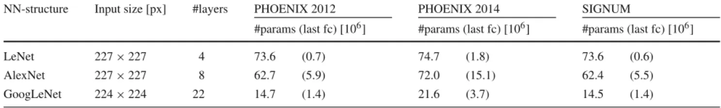
Table 3 Showing number of parameters (weights+biases) in millions of different CNN structures adapted to our tasks: PHOENIX 2012:1443 outputs PHOENIX 2014: 3694 outputs SIGNUM: 1366 outputs
NN-structure Input size [px] #layers PHOENIX 2012 PHOENIX 2014 SIGNUM
#params (last fc) [106] #params (last fc) [106] #params (last fc) [106]
LeNet 227×227 4 73.6 (0.7) 74.7 (1.8) 73.6 (0.6)
AlexNet 227×227 8 62.7 (5.9) 72.0 (15.1) 62.4 (5.5)
GoogLeNet 224×224 22 14.7 (1.4) 21.6 (3.7) 14.5 (1.4)
6.1 Effect of CNN Structure
A crucial research question is to estimate the effect of the CNN architecture on a specific task. This subsection aims to provide an answer to this question by applying different CNN structures to the task of sign language recognition, while all remaining hyper parameters are fixed (we adjust the transi-tion probabilities for each experiment). As such, we compare three well-known CNN architectures. All three have, at some point in time, received much attention by the community for outperforming the state-of-the-art largely on different classi-fication tasks. LeNet (full name is LeNet-5), introduced by LeCun et al. (1998), was the first successful CNN having 4 non-linear layers. Its application was character recogni-tion of the MNIST digits (LeCun et al.1998) with a size of 32×32 pixel. In this work, we employ a version which deviates from the original implementation by the number and kind of non-linearities. For simplicity we chose the version distributed jointly with the caffe framework (Jia et al.2014). The other two popular architectures analysed in the scope of this work were winners of the ImageNet Large Scale Visual Recognition Challenge (ILSVRC) in 2012 an 2014. AlexNet by Krizhevsky et al. (2012) was the first deeper CNN with 8 layers (5 convolutional and 3 fully connected layers). It won the object classification competition with a top-5 error of 15.4% across the targeted 1000 classes. Two years later Szegedy et al. (2015) won the competition with GoogLeNet. A 22-layer deep CNN that achieved a top-5 error of 6.67% on the task. In order to facilitate the comparison of the three mentioned architectures, we have compiled their key char-acteristics in Table3. Note that the number of parameters for GoogLeNet includes the parameters used for the two additional auxiliary softmax classifiers. Table3 shows the
input size, the number of non-linear layers and the number of parameters of the whole network (whose last output layers have been adjusted to each of the three data sets analysed in this work). It also shows the number of parameters of the last fully connected classification layer, which often makes up the largest part in the network and varies from task to task. The last layer’s size is due to the large amount of sign-labels
α(cfSect.3for details).αrepresents the labels belonging to the three hidden states that model each of the sign classes (over 1000) from our vocabulary (for PHOENIX 2014).
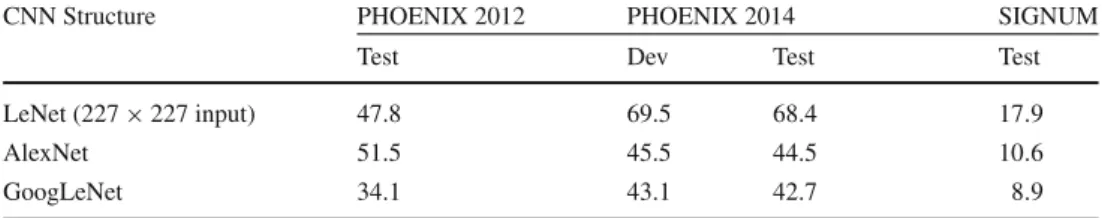
Discussion of Results Table 4 summarises the experi-mental results comparing the different CNN architectures. We see that GoogleNet clearly outperforms the other archi-tectures on both tasks with at least 4% relative improvement in WER. We further see that it is clearly not just the number of parameters that determines the model quality but rather the number of non-linear layers.
6.2 Effect of Finetuning
In this experiment we want to evaluate the effect of using out-of-domain data to train the networks prior to finetun-ing them on the actual in-domain task usfinetun-ing specific but quite limited training data. We therefore make use of the 1.2 million labelled images from the ILSVRC to train the networks. After that we exchange the final fully-connected classification layer and fine-tune the network. In case of the GoogLeNet architecture we exchange the layers of both aux-iliary classifiers as well. We perform the experiment with the AlexNet and the GoogLeNet architectures.
Discussion of results Tables5 and6 report the results for the AlexNet and GoogLeNet architecture, respectively. For both architectures out-of-domain training and subsequent
Table 4 Comparing different
CNN structures CNN Structure PHOENIX 2012 PHOENIX 2014 SIGNUM
Test Dev Test Test
LeNet (227×227 input) 47.8 69.5 68.4 17.9
AlexNet 51.5 45.5 44.5 10.6
GoogLeNet 34.1 43.1 42.7 8.9
Results in WER [%]: the lower the better
Table 5 Comparing the effect of pretraining CNN structures on out-of-task data: ILSVRC 2014
AlexNet PHOENIX 2012 PHOENIX 2014 SIGNUM
Test Dev Test Test
Randomly initialised 51.5 45.5 44.5 10.6
Fine-tuned 39.2 42.2 41.1 8.7
The first line represents training from scratch using the AlexNet structure, whereas the second corresponds to finetuning weights learnt on Imagenet. Results in WER [%]: the lower the better
Table 6 Comparing the effect of pretraining CNN structures on out-of-task data: ILSVRC 2014
GoogLeNet PHOENIX 2012 PHOENIX 2014 SIGNUM
Test Dev Test Test
Randomly initialised 34.1 43.1 42.7 8.9
Fine-tuned 30.0 38.3 38.8 7.4
The first line represents training from scratch using the GoogLeNet structure, whereas the second corresponds to finetuning weights learnt on Imagenet. Results in WER [%]: the lower the better
finetuning yields clear gains. With AlexNet we see 30% rel-ative improvement on PHOENIX 2012, 8% on PHOENIX 2014 and 20% on SIGNUM, while with GoogLeNet we see 13% relative improvement on PHOENIX 2012, over 10% on PHOENIX 2014 and again 20% on SIGNUM. We conclude that strongly supervised out-of-domain data has a consis-tently positive influence on learning hybrid sign language models—at least if the out-of-domain data is as diverse as ImageNet.
6.3 Hybrid Compared to Tandem Modelling
In this subsection we want to explore the question of whether it is better to use the CNN’s outputs as features and train a subsequent GMM-HMM system in the so-called tandem approach (Sect.3.3) or to directly use the posteriors as obser-vation probabilities as in the presented hybrid approach.
Discussion of resultsFigure9compares the hybrid CNN-HMM modelling against the tandem modelling. We can see that the hybrid approach slightly outperforms the tandem approach on all three data sets. This is consistent with the literature as found by Golik et al. (2013) in speech and hand-writing recognition. However, especially in terms of training complexity, the hybrid approach is clearly favourable as the subsequent GMM training is not necessary.
Fig. 9 The hybrid and the tandem approach side-by-side on all three data sets. Results in WER [%]: the lower the better
6.4 Effect of Hidden States
Until this point, we have seen experiments estimating the effect of several components on the overall sign recogni-tion pipeline. However, the quesrecogni-tion remains, how much the HMM impacts the final WER. It is clear that the HMM is the key element to allow the mapping from an input sequence of specific length to an output sequence of different length. But does the hidden state topology influence the final result in a similar way as the CNN structure or the CNN training?
In this subsection we analyse the effect of the HMM struc-ture. More specifically, we want to know if multiple hidden states help the deep CNN to perform better or if they are a relic of the GMM-HMM architecture that strong CNNs make redundant. Therefore, we perform experiments on the
Fig. 10 Showing the best achieved WERs in [%] (the lower the better) on PHOENIX 2014 for different numbers of states and repetitions
PHOENIX 2014 data set altering the HMM topology w.r.t. the number of hidden states. The baseline system corresponds to a HMM architecture that models each sign-word with 3 hidden states which are each repeated twice (sharing the same probabilities). Thus, this topology has 6 states, but only 3 probability distributions need to be estimated by the CNN. This standard bakis topology ensures that we can compensate for variation in signing speed by skipping states. By defini-tion, we can skip at most one state. The repetitions therefore ensure that all emission probabilities have to be visited at least a single time. In order to allow for valid conclusions, we need to make sure that all systems have the chance to find a good alignment w.r.t. their HMM architecture. In opposition to all other experiments presented in the scope of this work, we therefore perform multiple iterations of re-alignment, where we re-estimate the viterbi path. We start from a flat segmen-tation, where the available frames are equally distributed across all states of a sentence. The re-alignment then iter-atively updates the frame labelling and therefore affects the subsequent CNN training. Thus, after each re-alignment we perform a fine-tuning of the previous iteration’s model for 100k iterations (∼4 epochs). Each iteration takes about 6 h for CNN training and 20 minutes for viterbi alignment. We perform 10 re-alignment iterations for all different HMM topologies and report the best result among all iterations.
Discussion of resultsFigure10shows the results in terms of WER on the PHOENIX 2014 dev and test partition. We first vary the amount of states per sign-word from 1 to 8, main-taining the 2 state repetitions. In this setting, the baseline of 3 states and 2 repetitions clearly outperforms topologies with less states. However, we see the best performance further increasing the numbers of states to 7. We note a WER dif-ference between the weakest (1×2 states) and the strongest topology (7×2 states) of 8.5% absolute and over 20% rel-ative. The 7 state architecture achieves 33.4% WER on the dev set and 34.4 on the test set. One could argue that it is the implied HMM length and not the division into hidden states that produces the improvements with longer HMMs. Therefore, we further perform an experiment with 1 state and 6 repetitions, which has the same length behaviour as the
Table 7 Showing how the HMM structure in terms of HMM states and repetitions affects the total number of HMM states and the neural network parameters (weights+biases) in millions
HMM structure PHOENIX 2014
States×Repetitions Total states Parameters [106]
1×2 1232 14.1 2×2 2463 17.9 3×2 3694 21.7 4×2 4925 25.4 5×2 6156 29.2 6×2 7387 33.0 7×2 8618 36.8 8×2 9849 40.6
baseline. However, this model performs much worse than the baseline. As such, we can conclude that the HMM architec-ture has a strong influence on the recognition performance. Nevertheless, in Table 7 we can see how the number of HMM states affects the overall model size. This significantly impacts runtime.
6.5 Effortless Ensemble of Models
Finally, we want to show that a log-linear combination of multiple CNN models can further improve performance. We therefore define the probability by the visual model to be the combined product of each single modeli scaled by a factor
δias in px1T|w1N=max sT 1 T t=1 i p i(α|xt) pi(α)β δi ·pst|st−1, w1N (16)
In the scope of this work we combine I = 2 mod-els. The fact that model ensembles increase performance is well known. However, typically the building of models that are sufficiently complementary to yield any improve-ments constitutes a large computational overhead. In this section, we show that the process of re-aligning the mod-els already adds sufficient discriminative information. Even models from successive re-alignment iterations yield strong gains when deployed as ensemble. This is remarkable as it means that with the proposed algorithm we get such models free of additional effort.
We choose two successive iterations of the best HMM architecture using 7 states and 2 repetitions, namely the 10th iteration yielding 33.6/34.6 and the 9th iteration yield-ing 33.8/34.6 on the development set and on the test set respectively. The log-linear combination withδ1=0.87 and
δ2 =0.13 yields a WER of 31.6% and 32.5% for dev and test respectively on PHOENIX 2014. This corresponds to a
Fig. 11 Showing the best achieved WERs in [%] (the lower the better) on PHOENIX 2014 for log-linear model combination of the two best alignment iterations (while keeping the HMM architecture fixed)
relative gain of around 6% compared to the single models (Fig.11).
6.6 General Comparison to State-of-the-Art
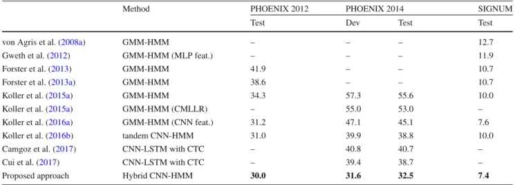
Table8shows a detailed comparison to the state-of-the art on the three employed benchmark corpora. Besides per-formance measures, it reports the method of choice by the respective publications. Note that the proposed hybrid approach currently exploits only a single cropped hand of the signer and yet achieves state-of-the-art performance. Sign language is highly multimodal and makes heavy use of manual components (hand shape, orientation, place of artic-ulation, movement) and also non-manual components (facial expression, eyebrow height, mouth, head orientation, upper body orientation). Most of the competing approaches use these additional modalities in recognition, which is why we expect additional gain when including them in the proposed approach. The previously best hand only result mentioned in Koller et al. (2016a) also relied on CNN models, but did not employ the hybrid approach end-to-end in recog-nition, loosing some performance due to this. It set the benchmark on PHOENIX 2014 Multisigner to 51.6% WER. However, our proposed CNN-HMM achieves a strong result of 33.6% and 34.6% on dev and test respectively with a single model and 31.6%/32.5% with model combination. This corresponds to about 20% absolute WER or over 38% relative improvement. On the single signer corpus RWTH-PHOENIX-Weather 2012 the proposed approach improved the best baseline from 35.5% to 30.0%, still being a relative improvement of over 15%. On SIGNUM we improve the best known word error rates from from 12.0% to 7.4%. As can be seen in Table8, our hand-only hybrid CNN-HMM even outperforms multimodal approaches.
Nevertheless, the need to include more modalities than just the right hand is revealed by looking at the recogni-tion errors. Qualitative examinarecogni-tion of the top confusions on PHOENIX 2014 made by the hybrid approach highlight con-fused pairs such as “SNOW” with “RAIN” or “SHOWER”
with “RAIN”. However, these signs share the same hand con-figurations, whereas only the mouth shape changes. Given the classification relies purely on the right hand, it is understand-able that it cannot distinguish between these signs. The top 30 confusions all relate to this type of error.
7 Conclusion and Future Work
In this work, we introduced an end-to-end embedding of a CNN into a HMM, while interpreting the outputs of the CNN in a truly Bayesian framework and training the system as a hybrid CNN-HMM in an end-to-end fashion Most state-of-the-art approaches in gesture and sign language modelling use a sliding window approach or simply evaluate the out-put in terms of overlap with the ground truth. While this is sufficient for data sets that provide such training and evalua-tion characteristics, it is unsuitable for real world use. For the field to move forward more realistic scenarios, such as those imposed by challenging real-life sign language corpora, are required.
In this manuscript, we presented a hybrid CNN-HMM framework that combines the strong discriminative abilities of CNNs with the sequence modelling capabilities of HMMs, while abiding to Bayesian principles. This work represents the extended version of our previous work (Koller et al. 2016b), where we were the first to present such an embedding in the context of sign language and gesture recognition.
With the hybrid method we were able to achieve a large relative improvement of over 15% compared to the previous state-of-the-art on three challenging benchmark continuous sign language recognition data sets. On the two single signer data sets RWTH-PHOENIX-Weather 2012 and SIGNUM we improve the best known word error rates from 35.5 to 30.0% and from 12.0 to 7.4% respectively, while only employ-ing basic hand-patches as input. On the difficult 9 signer
>1000 vocab RWTH-PHOENIX-Weather 2014 Multisigner, we lower the error rates from 51.6%/50.2% to 31.6%/32.5% on dev/test.
In the scope of this extended manuscript, we significantly added to the theoretical explanation of the hybrid approach, with the aim of making its idea more accessible to newcomers to the field and presented much more extensive experiments: We analysed the effect of both CNN- and HMM-structure on the hybrid approach. We investigated the effect of using out-of-domain data to train the network prior to finetuning using in-domain data. Finally, we showed that the use of ensembles of hybrid CNN-HMMs is able to further boost performance. In terms of future work, we would like to extend our approach to cover all relevant modalities. Moreover, tech-niques to overcome the necessary initial alignment, such as end-to-end training will also be investigated.
Table 8 Comparison with state-of-the-art
Method PHOENIX 2012 PHOENIX 2014 SIGNUM
Test Dev Test Test
von Agris et al. (2008a) GMM-HMM – – – 12.7
Gweth et al. (2012) GMM-HMM (MLP feat.) – – – 11.9
Forster et al. (2013) GMM-HMM 41.9 – – 10.7
Forster et al. (2013a) GMM-HMM 38.6 – – 10.7
Koller et al. (2015a) GMM-HMM 34.3 57.3 55.6 10.0
Koller et al. (2015a) GMM-HMM (CMLLR) – 55.0 53.0 –
Koller et al. (2016a) GMM-HMM (CNN feat.) 31.2 47.1 45.1 7.6
Koller et al. (2016b) tandem CNN-HMM 31.0 39.9 38.8 10.0
Camgoz et al. (2017) CNN-LSTM with CTC – 40.8 40.7 –
Cui et al. (2017) CNN-LSTM with CTC – 39.4 38.7 –
Proposed approach Hybrid CNN-HMM 30.0 31.6 32.5 7.4
Best results are highlighted in bold
Results in WER [%]: the lower the better. Best results of the proposed approach are single models. Model combination further improves the error on PHOENIX 2014 down to 34.4%
Open Access This article is distributed under the terms of the Creative Commons Attribution 4.0 International License (http://creativecomm ons.org/licenses/by/4.0/), which permits unrestricted use, distribution, and reproduction in any medium, provided you give appropriate credit to the original author(s) and the source, provide a link to the Creative Commons license, and indicate if changes were made.
References
Assael Y. M., Shillingford, B., Whiteson, S., & de Freitas, N. (2016).
LipNet: End-to-end sentence-level lipreading.arXiv:1611.01599
Bahl, L. R., Jelinek, F., & Mercer, R. L. (1983). A maximum likelihood approach to continuous speech recognition.IEEE Transactions on Pattern Analysis and Machine Intelligence,PAMI–5(2), 179–190.
https://doi.org/10.1109/TPAMI.1983.4767370.
Bakis, R. (1976). Continuous speech recognition via centisecond acous-tic states.The Journal of the Acoustical Society of America,59(S1), S97–S97.https://doi.org/10.1121/1.2003011.
Bengio, Y., & Frasconi, P. (1996). Input–output HMMs for sequence processing.IEEE Transactions on Neural Networks,7(5), 1231– 1249.
Bluche, T., Ney, H., Louradour, J., & Kermorvant, C. (2015). Framewise and CTC training of neural networks for handwriting recogni-tion. In2015 13th international conference on document analysis and recognition (ICDAR) (pp. 81–85).https://doi.org/10.1109/ ICDAR.2015.7333730
Bourlard, H., & Wellekens, C. J. (1989). Links between Markov models and multilayer perceptrons. In Advances in neural information processing systems(pp. 502–507).
Bourlard, H. A., & Morgan, N. (1993).Connectionist speech recog-nition: A Hybrid approach. Norwell, MA: Kluwer Academic Publishers.
Camgoz, N. C, Hadfield, S., Koller, O., & Bowden, R. (2017). Sub-UNets: End-to-end hand shape and continuous sign language recognition. InIEEE international conference on computer vision
(pp. 22–27).
Cui, R., Liu, H., & Zhang, C. (2017). Recurrent convolutional neural networks for continuous sign language recognition by staged opti-mization. InThe IEEE conference on computer vision and pattern recognition (CVPR), Honolulu, HI, USA.
Dreuw, P., Deselaers, T., Rybach, D., Keysers, D., & Ney, H. (2006). Tracking using dynamic programming for appearance-based sign language recognition. InIEEE international conference automatic face and gesture recognition(pp. 293–298). Southampton: IEEE. Escalera, S., Baró, X., Gonzalez, J., Bautista, M. A, Madadi, M., Reyes, M., et al.. (2014). Chalearn looking at people challenge 2014: Dataset and results. InComputer vision-ECCV 2014 workshops
(pp. 459–473). Springer.
Forster, J., Schmidt, C., Hoyoux, T., Koller, O., Zelle, U., Piater, J., et al. (2012). RWTH-PHOENIX-weather: A large vocabulary sign language recognition and translation corpus. In:International con-ference on language resources and evaluation, Istanbul, Turkey (pp. 3785–3789).
Forster, J., Koller, O., Oberdörfer, C., Gweth, Y., & Ney, H. (2013a). Improving continuous sign language recognition: Speech recog-nition techniques and system design. InWorkshop on speech and language processing for assistive technologies, Grenoble, France. Satellite workshop of INTERSPEECH 2013 (pp. 41–46). Forster, J., Oberdörfer, C., Koller, O., & Ney, H. (2013b). Modality
combination techniques for continuous sign language recognition. InIberian conference on pattern recognition and image analysis. Lecture Notes in Computer Science 7887 (pp. 89–99). Madeira: Springer.
Forster, J., Schmidt, C., Koller, O., Bellgardt, M., & Ney, H. (2014). Extensions of the sign language recognition and translation cor-pus RWTH-PHOENIX-weather. InInternational conference on language resources and evaluation, Reykjavik, Island (pp. 1911– 1916).
Golik, P., Doetsch, P., & Ney, H. (2013). Cross-entropy vs. squared error training: A theoretical and experimental comparison. In INTER-SPEECH(pp. 1756–1760).
Granger, N., el Yacoubi, M. A (2017). Comparing hybrid NN-HMM and RNN for temporal modeling in gesture recognition. In Neu-ral information processing. Lecture Notes in Computer Science (pp. 147–156). Cham: Springer. https://doi.org/10.1007/978-3-319-70096-0_16.
Graves, A., & Schmidhuber, J. (2005). Framewise phoneme clas-sification with bidirectional LSTM and other neural network architectures.Neural Networks,18(5), 602–610.
Gweth, Y., Plahl, C., & Ney, H. (2012). Enhanced continuous sign language recognition using PCA and neural network features. In
CVPR 2012 workshop on gesture recognition, Providence, Rhode Island, USA (pp. 55–60).
Hermansky, H., Ellis, D.W, & Sharma, S. (2000). Tandem connection-ist feature extraction for conventional HMM systems. In2000 IEEE international conference on acoustics, speech, and signal processing, 2000(Vol. 3, pp. 1635–1638). ICASSP’00. Proceed-ings. IEEE.
Huang, J., Zhou, W., Li, H., & Li, W. (2015). Sign language recog-nition using 3D convolutional neural networks. In 2015 IEEE international conference on multimedia and expo (ICME)(pp. 1– 6).https://doi.org/10.1109/ICME.2015.7177428.
Jia, Y., Shelhamer, E., Donahue, J., Karayev, S., Long, J., Girshick, R., et al. (2014).Caffe: Convolutional architecture for fast feature embedding. CoRRarXiv:1408.5093.
Koller, O., Forster, J., & Ney, H. (2015a). Continuous sign lan-guage recognition: Towards large vocabulary statistical recog-nition systems handling multiple signers. Computer Vision and Image Understanding, 141, 108–125. https://doi.org/10.1016/j. cviu.2015.09.013.
Koller, O., Ney, H., & Bowden, R. (2013). May the force be with you: force-aligned signwriting for automatic subunit annotation of corpora. InIEEE international conference on automatic face and gesture recognition, Shanghai (pp. 1–6).
Koller, O., Ney, H., & Bowden, R. (2014). Read my lips: Continu-ous signer independent weakly supervised viseme recognition. In
Proceedings of the 13th European conference on computer vision, Zurich (pp. 281–296).
Koller, O., Ney, H., & Bowden, R. (2015b). Deep learning of mouth shapes for sign language. InThird workshop on assistive computer vision and robotics. Santiago: ICCV.
Koller, O., Ney, H., & Bowden, R. (2016a). Deep hand: How to train a CNN on 1 million hand images when your data is continuous and weakly labelled. InIEEE conference on computer vision and pattern recognition, Las Vegas, NV, USA (pp. 3793–3802). Koller, O., Zargaran, S., Ney, H., & Bowden, R. (2016b). Deep sign:
Hybrid CNN-HMM for continuous sign language recognition. In
British machine vision conference, York, UK.
Koller, O., Zargaran, S., & Ney, H. (2017). Re-sign: Re-aligned end-to-end sequence modelling with deep recurrent CNN-HMMs. In
IEEE conference on computer vision and pattern recognition, Hon-olulu, HI, USA.
Krishnan, R., & Sarkar, S. (2015). Conditional distance based match-ing for one-shot gesture recognition.Pattern Recognition,48(4), 1298–1310.
Krizhevsky, A., Sutskever, I., & Hinton, G. E. (2012). ImageNet classi-fication with deep convolutional neural networks. InAdvances in neural information processing systems(pp. 1106–1114). Le, H. S., Pham, N. Q., & Nguyen, D. D. (2015). Neural networks with
hidden Markov models in skeleton-based gesture recognition. In V. H. Nguyen, A. C. Le, & V. N. Huynh (Eds.),Knowledge and systems engineering. Advances in Intelligent Systems and Com-puting(Vol. 326, pp. 299–311). Cham: Springer.https://doi.org/ 10.1007/978-3-319-11680-8_24.
LeCun, Y., Bottou, L., Bengio, Y., & Haffner, P. (1998). Gradient-based learning applied to document recognition.Proceedings of the IEEE,86(11), 2278–2324.
Marcel, S., Bernier, O., Viallet, J.E, & Collobert, D. (2000). Hand gesture recognition using input–output hidden Markov models. InFourth IEEE international conference on automatic face and gesture recognition, 2000. Proceedings (pp. 456–461). IEEE. Molchanov, P., Gupta, S., Kim, K., & Kautz, J. (2015). Hand gesture
recognition with 3D convolutional neural networks. In Proceed-ings of the IEEE conference on computer vision and pattern recognition workshops(pp. 1–7).
Neverova, N., Wolf, C., Taylor, G.W, & Nebout, F. (2014). Multi-scale deep learning for gesture detection and localization. In L. Agapito,
M. M Bronstein, & C. Rother (Eds.),Computer vision—ECCV 2014 workshops. Lecture Notes in Computer Science (pp. 474– 490). Springer.https://doi.org/10.1007/978-3-319-16178-5_33. Ney, H., & Ortmanns, S. (2000). Progress in dynamic programming
search for LVCSR.Proceedings of the IEEE,88(8), 1224–1240. Ong, E. J., Koller, O., Pugeault, N., & Bowden, R. (2014). Sign
spot-ting using hierarchical sequential patterns with temporal intervals.
IEEE Conference on Computer Vision and Pattern Recognition
(pp. 1931–1938). OH, USA: Columbus.
Pigou, L., van den Oord, A., Dieleman, S., Van Herreweghe, M., & Dambre, J. (2018). Beyond temporal pooling: Recurrence and temporal convolutions for gesture recognition in video.
International Journal of Computer Vision,126(2–4), 430–439.
arXiv:1506.01911.
Rao, Y., Lu, J., & Zhou, J. (2017). Attention-aware deep reinforcement learning for video face recognition. InProceedings of the IEEE conference on computer vision and pattern recognition(pp. 3931– 3940).
Richard, A., Kuehne, H., & Gall, J. (2017). Weakly supervised action learning with RNN based fine-to-coarse modeling. InIEEE con-ference on computer vision and pattern recognition, Hawaii, USA.
arXiv:1703.08132.
Richard, M. D., & Lippmann, R. P. (1991). Neural network classifiers estimate Bayesian a posteriori probabilities.Neural Computation,
3(4), 461–483.
Rybach, D., Hahn, S., Lehnen, P., Nolden, D., Sundermeyer, M., Tüske, Z., et al. (2011). RASR—The RWTH Aachen University open source speech recognition toolkit. InIEEE automatic speech recognition and understanding workshop, Waikoloa, HI, USA. Schlüter, R., Nussbaum-Thom, M., & Ney, H. (2012). Does the cost
function matter in Bayes decision rule?IEEE Transactions on Pat-tern Analysis and Machine Intelligence,34(2), 292–301.https:// doi.org/10.1109/TPAMI.2011.163.
Schober, M., Adam, A., Yair, O., Mazor, S., & Nowozin, S. (2017). Dynamic time-of-flight. In The IEEE conference on computer vision and pattern recognition (CVPR).
Stolcke, A. (2002). SRILM—An extensible language modeling toolkit. InProceedings on international conference on spoken language processing (ICSLP), Denver, Colorado.
Szegedy, C., Liu, W., Jia, Y., Sermanet, P., Reed, S., Anguelov, D., et al. (2015). Going deeper with convolutions. InThe IEEE conference on computer vision and pattern recognition (CVPR), Boston, MA (pp. 1–9).
von Agris, U., Knorr, M., & Kraiss, K.F (2008a). The significance of facial features for automatic sign language recognition. In8th IEEE international conference on automatic face & gesture recog-nition, 2008. FG’08 (pp. 1–6). IEEE.
von Agris, U., Zieren, J., Canzler, U., Bauer, B., & Kraiss, K. F. (2008b). Recent developments in visual sign language recognition. Univer-sal Access in the Information Society,6(4), 323–362.
Wu, D., Pigou, L., Kindermans, P. J., Le, N., Shao, L., & Dambre, J. (2016). Deep dynamic neural networks for multimodal gesture seg-mentation and recognition.IEEE Transactions on Pattern Analysis and Machine Intelligence,38(8), 1583–1597.
Wu, D., & Shao, L. (2014). Deep dynamic neural networks for gesture segmentation and recognition. InComputer vision—ECCV 2014 workshops(pp. 552–571). Springer.
Publisher’s Note Springer Nature remains neutral with regard to juris-dictional claims in published maps and institutional affiliations.
![Fig. 10 Showing the best achieved WERs in [%] (the lower the better) on PHOENIX 2014 for different numbers of states and repetitions](https://thumb-us.123doks.com/thumbv2/123dok_us/1073508.2642864/12.892.78.434.78.249/showing-achieved-better-phoenix-different-numbers-states-repetitions.webp)
![Fig. 11 Showing the best achieved WERs in [%] (the lower the better) on PHOENIX 2014 for log-linear model combination of the two best alignment iterations (while keeping the HMM architecture fixed)](https://thumb-us.123doks.com/thumbv2/123dok_us/1073508.2642864/13.892.81.431.77.249/showing-achieved-phoenix-combination-alignment-iterations-keeping-architecture.webp)