The Research Data Centres
Information and Technical Bulletin
Spring 2006, vol. 3 no. 1
Statistics Statistique Canada Canada
Merging area-level census data with survey data in Statistics Canada
Research Data Centres
By Denis Gonthiera, Tina Hottonb, Cynthia Cookc, and Russell Wilkinsd
Abstract
This article explains how to append census area-level summary data to survey or administrative data. It uses examples from datasets present in Statistics Canada Research Data Centres, but the methods also apply to external datasets. Four examples illustrate common situations faced by researchers: (1) when the survey (or administrative) and census data both contain the same level of geographic identifiers, coded to the same year standard ("vintage") of census geography; (2) when the two files contain geographic identifiers of the same vintage, but at different levels of census geography; (3) when the two files contain data coded to different vintages of census geography; (4) when the survey data are lacking in geographic identifiers, and those identifiers must first be generated from postal codes present on the file. The examples are shown using SAS syntax, but the principles apply to other programming languages or statistical packages.
Introduction
Over the past decade, interest in the effect of neighbourhood characteristics on child development, health, crime and many other social outcomes has resurfaced among social scientists in Canada (Boyle and Lipman, 1998; Boyle and Willms, 1999, Roos et al., 2004; Ross et al., 2004, and Soubhi et al., 2001) and elsewhere. This resurgence is, in part, due to the widespread availability of statistical software for modeling hierarchically-clustered data. In Canada, the availability of large-scale national surveys with detailed geographic identifiers, which can be accessed through the Research Data Centre (RDC) program, has also played a role in the renewed interest in conducting neighbourhood-related research.
Researchers may be interested in the “contextual effects” which emerge from within-neighbourhood social interactions, and/or the “integral effects” emerging from the local material environment (such as toxic dumps, factories, or parks) (Oakes, 2004). Although there is certainly no consensus on how neighbourhoods should be defined, many researchers in Canada are turning to Canadian census profile data as a source of information to measure the contextual effects of local communities. Census profile data contain the socio-demographic characteristics of geographic areas, including variables relating to population structure, ethnic composition, employment and income. The lowest level of geography available in these profiles, and arguably
a. Corresponding author: Denis Gonthier, Analyste principal, Centre interuniversitaire québécois de statistiques sociales (CIQSS) - Université de Montréal, 3535, chemin Queen-Mary, bureau 420, Montréal, Québec, H3V 1H8, Telephone: 1-514-343-2090 poste 3, Fax: 1-514-343-2328, Email: [email protected]
b. Statistics Canada, Research Data Centre Program, University of Toronto c. Statistics Canada, Research Data Centre Program, University of Western Ontario
the closest to meaningful neighbourhoods, is the dissemination area (DA) – previously known as enumeration area (EA) – or for larger urban centres, the somewhat larger census tract (CT).1
The DA is a small, relatively stable geographic unit composed of one or more census blocks (CB). It is the smallest standard geographic area for which census data are disseminated, targeting from 400 to 700 persons to avoid data suppression (Statistics Canada, 2000).2 As of the 2001 census, the DA replaces the EA as the basic unit for data dissemination. CTs are relatively stable geographic areas, typically containing between 2,500 and 8,000 (average 4,000) residents; they are only defined in census metropolitan areas (CMAs) and census agglomerations (CAs) with an urban core population of 50,000 or more in the preceding census.3 Consequently, CTs are only appropriate for research with an intra-urban focus. (For a brief explanation of the various levels of census geography, plus their common acronyms, see Appendix 1.)
Most of the Statistics Canada surveys available at RDCs across the country contain geographic identifiers that enable researchers to merge the survey data with aggregate census profile data; however, researchers may encounter some difficulties, as a full compliment of geographic identifiers may not be available on each of the microdata files. Another common challenge of merging these data is that the "vintage," or year of the particular census for which
the geographic identifiers were defined, may not be ideal for the time period under analysis.
This article provides step-by-step instructions on how to merge census EA or DA and CT profile data with Statistics Canada survey microdata files. We explore several different situations in which geographic identifiers are available in Statistics Canada microdata files, and highlight the importance of taking the vintage of the geographic codes into consideration.
Specifically, we deal with four scenarios. (1) The first example applies when the geographic identifier used in a given census profile is identical to the geographic identifier available on the survey microdata file. We explain how to do a direct merge of 2001 aggregate census data and data from the 2003 Canadian Community Health Survey Cycle 2.1 (CCHS 2.1), using the DA identifier. (2) The second example pertains to cases where the two files contain geographic identifiers of the same vintage, but at different levels of census geography. For the CCHS 2.1 data, the 2001 DA is available, but not the 2001 CT. In this case, an intermediate step is required to obtain the correspondence between the 2001 DA and 2001 CT, using a Geography Tape File (GTF). (3) The third example is useful when the two files contain data coded to different vintages of census geography. For example, the CCHS Cycle 1.2 contains geographic codes based on the 1996 census, but researchers may be more interested in linking to 2001 census profile data, given that the survey data were collected in 2002. In such cases, a preliminary merge permits "translating" between the two vintages of census geography. (4) The fourth and final example is applicable when the survey data are lacking in geographic identifiers, and those identifiers must first be generated from postal codes present on the file, using the
1. To obtain resource materials on Canadian census geography, visit
http://geodepot.statcan.ca/Diss/Reference/Reference_e.cfm.
2. DAs respect the boundaries of census subdivisions (CSDs) and CTs. DAs stay stable over time to the extent that CSDs and CTs do. It is possible to find DAs with population counts lower that 400 or higher than 700, usually resulting from an attempt to respect CSD and CT boundaries.
3. Note that once a CMA or CA has been divided into CTs, the CTs are maintained even if the urban core population subsequently declines below 50,000 (Statistics Canada, 2004).
Postal Code Conversion File (PCCF or PCCF +). For the case of the National Population Health Survey (NPHS) Cycle 3 data, collected in 1998-1999, we explain how to use the PCCF+ to obtain a full repertoire of geographic variables that can then be used to merge the survey data with census profile data.
II. Example 1. Merging when the same level and vintage of geographic identifier is available on each file
This section presents a relatively simple example of merging. This occurs when the survey data are coded with the same level and same vintage of geographic variables as the census profiles of interest. To illustrate that scenario, we use a recent cross-sectional dataset available in the RDCs: Cycle 2.1 of the Canadian Community Health Survey (CCHS 2.1). The data for this survey were collected during the period January 2003 to November 2003. The most recent source of contextual variables for that source is the 2001 census.
The CCHS 2.1 dataset includes the 2001 DA, which is also present on the 2001 census DA profiles. For readers not familiar with the conventions of census geography, it is important to note that a geographic code such as a DA is composed of several elements and always has a specific vintage. The DA unique identifier (DAuid) includes the following three components: a two-digit region plus province or territory code (PR); a two-digit census division code (CD); and a four-digit DA. In addition, all census geographic codes have a vintage, which refers to the particular census standard for which they were defined. This applies to DAs as well as to all other census geographic identifiers such as CMA or CT. In the present case, we are dealing with 2001 census geography, so we will assign the variable name DA01uid to the full eight-digit DA unique identifier (PR(2)+CD(2)+DA(4), all based on 2001 census geography).
In order to link the CCHS 2.1 dataset with the census profile dataset, we merge the two datasets by the variable representing the DA01uid (which is called GEOCDDA in the CCHS 2.1 dataset, and DAuid on the census profile dataset). For the proper observations to be linked during the merge, the "by" variables must have exactly the same variable name and format. In this example we use the variable name DA01uid, which as just noted, is composed of PR(2)+CD(2)+DA(4). Although the form may appear numeric, it is preferable to use character formats for all geographic identifiers. One reason is that the leading zeros have an importance: DA ‘0024’ is not the same as DA ’24’. Character format also allows easy extraction of the higher-level geographic codes for a given DAuid. In the current case, both variables must have a length of 8 digits (characters) to permit the merge to be successful. It is always a good idea to first browse the datasets (sorted by the merge "by" variable, in this case DA01uid) to ensure the coding is consistent across the two datasets.
The following SAS syntax (see Figure 1) can be used to create an 8-character alphanumeric variable called DA01uid, from an 8-digit numeric source variable called GEOCDDA.
Figure 1 DA01uid=put(GEOCDDA, 8.);
Before doing the merge, SAS requires that the two datasets (containing the CCHS variables and the 2001 census DA profile variables) be sorted by the same variable, in this case DA01uid. This being done, one can perform the merge of the census profiles and survey data. Researchers should avoid duplication of variable names across data sets used in merges, so as to prevent the values of one dataset from overriding the values of the other dataset. The only exception to this is of course the "by" variable name used for the merge, which must be the same on both datasets.
Here is an example of SAS syntax used for merging the two datasets:
Figure 2
/* Example 1. */
/* SAS syntax for merging when the survey and census data */ /* both contain the same level of geographic identifiers, */ /* coded to the same vintage of census geography */
libname source 's:\cchs';
libname final 's:\cchs\results';
/* get the subset of CCHS variables required: */
data cchs (keep= DA01uid dhhc_age dhhc_sex genc_01 genc_07); set source.cchsmain;
DA01uid=put(GEOCDDA, 8.); Label dhhc_age = ‘Age’
dhhc_sex = ‘Sex’
genc_01 = ‘Self-perceived health’ genc_07 = ‘Self-perceived stress’
; run;
/* now get the 2001 DA profile data needed: */
data daprofil (keep=DA01uid v80 v400 v404 v916 v1442); set source.da_federal_2001_profile;
DA01uid=DAuid;
Label v80 = ‘Average number of children at home per census family’ v400 = ‘Total population by immigrant status and place of birth’ v404 = ‘Total immigrants by selected places of birth’
v916 = ‘Unemployment rate’
v1442 = ‘Median 2000 household income $’ ;
run;
/* prepare for the merge by sorting both datasets the same way: */ proc sort data=cchs; by DA01uid;
proc sort data=daprofil nodupkey; by DA01uid;
/* merge the two datasets by the common "by" variable: */ data combined missed outside;
merge cchs (in=a) daprofil (in=b); by DA01uid;
if a and b then output combined;
else if a and not b then output missed; else if b and not a then output outside;
run;
set combined missed; /* records with missing values for DA01uid are retained, as are records with missing DA profile data */
run;
Using two dichotomous flags (measuring inclusion of records with “in” variables A and B), this program creates three different SAS datasets. The dataset COMBINED includes the observations of the CCHS 2.1 file that also have a matching DA record in the DAPROFIL dataset.4 The dataset MISSED consists of cases where the CCHS respondents do not have a corresponding record in the DAPROFIL dataset (the DA is not included in those records). Finally, the OUTSIDE dataset is the list of DAs that are not covered by the CCHS 2.1 survey. Note that this information is confidential, as it allows one to deduce the list of DAs that are selected in the CCHS survey. We create a permanent version of the concatenated datasets COMBINED and MISSED, called NEWCCHS. For analytical purposes, it is important to also retain the MISSED records, since they just have missing values for the census variables (sometimes for important analytical reasons). Missing values can be excluded later - preferably after the examination of the other characteristics of those records with no information from the census profiles.
From the 135,573 records present in the CCHS 2.1 dataset, 134,550 (those in the COMBINED dataset) were successfully merged to the census profile dataset. An additional 1,023 CCHS 2.1 respondents (those in the MISSED dataset) had a 2001 DA that we did not find in this particular 2001 census profile,5 so the contextual variables derived from this profile are not available for them. Those cases represent only 0.8% of the observations. The most common reason for not finding a match in the census profile is because the DAs in question have too small a population. For confidentiality reasons, census profile data are only available for areas with a population of 40 or greater, and income data are not shown unless the DA has a non-institutional population of 250 or more, so income data are more frequently missing than are variables from the "series A" population data (such as mother tongue).
III. Example 2. Merge of data requiring inference between different levels of geography (but where both the census and survey data have the same vintage of census geography)
For this example, we will continue to use CCHS 2.1 data. This time, we wish to add 2001 CT data. Since CTs are only defined for CMAs and larger CAs, the analysis is limited to urban Canada. The problem is that, in the case of CCHS 2.1 data, the DA is available (in a variable called GEOCDDA), but not the CT. So, the use of the 2001 CT profiles requires an intermediate step to produce a correspondence between the 2001 DA and 2001 CT.6 Figure 3 provides a summary of the data files needed and the geographic variables involved.
4. For the census variables of interest to us, we create a subset called DAPROFIL. The full set of census variables in the RDC is present in the SAS dataset DA_FEDERAL_2001_PROFILE.
5. More DAs are included in the profiles based on census short questionnaire (A series) than in the profiles from the census long questionnaire (B series). Within the B series, income variables may have missing values while other variables such as education may not be missing.
6. It is relatively easy to do the DA to CT correspondence by using one of a series of Geography Tape Files (GTF)- one for each census year from 1971 to 2001, abstracted in standardized format from the full GTF, Geography Attributes Files, GeoRef 1996, or GeoSuite 2001. The GTF files can be obtained in the Research Data Centres. They each appear as a flat file and have a record layout that can be used to read the data into SAS.
Figure 3
Geographic level Variable names on each data file
CCHS 2.1 file (vintage 2001 census geography) 2001 GTF (vintage 2001 census geography) 2001 CT profiles (vintage 2001 census geography) DA GEOCDDA DAUID -CT - CMA + CT CTUID
The first step is to merge the CCHS 2.1 dataset with the 2001 GTF dataset, in order to add a CT7 to the CCHS 2.1 data. This will be done using a DA that needs to have the same variable name and format in both datasets. As we saw in section II, the CCHS 2.1 data contain a variable GEOCDDA that is numeric. This should be changed to an alphanumeric variable called DA01uid. The variable present in the GTF dataset is already defined as alphanumeric, but the variable name DAuid should be changed to DA01uid (to agree with the CCHS 2.1 variable name, which to be clear, includes the census year as part of the variable name).
The 2001 GTF (gtf01da.can) may be read in using this SAS syntax:
Figure 4
filename gtf01da 's:\cchs\gtf01da.can';
data gtf01da (keep=da01uid ct01uid); infile gtf01da;
length CT01uid $ 10 zero $ 1; input
@ 1 da01uid $char8. /* pr(2)+cd(2)+da(4) */
@ 27 cma $char3. /* cma or ca incl 996-999 miz */ @ 31 ct $char6. /* census tract */
/* to get pure CMA/CA codes, eliminate the MIZ codes: */ if cma in ('996' '997' '998' '999') then cma='000'; ;
zero='0';
CT01uid=cma||zero||ct; run;
The above syntax (Figure 4) reads in only those variables from the GTF file which are needed for the merge to the 2001 census profiles. It includes a DA01uid variable plus two variables (CMA and CT) that are then concatenated to form a full and unique 2001 CT, called CT01uid.
7. Many in-house products from the Geography Division of Statistics Canada use the term "CT code" to refer to a 4 digit code for internal use within Statistics Canada, while the term "CT name" is used for what everybody else refers to, somewhat loosely, as the "CT code". To avoid confusion, we will simply refer to "CT name" as CT.
To agree exactly with the CT01uid variable present in the 2001 census profile dataset, CT01uid is created by combining a three-digit CMA/CA and a seven-digit CT. The CT itself has 7 digits: a four digit section, plus a decimal point and two places after the decimal (for example: 0042.00). If a CT is split into two or more parts due to a population increase, the number after the decimal point identifies the split. For example, CT 0042.00 could be split into CT 0042.01 and CT 0042.02. Notice that CTs also have a vintage, so the census year should always be specified in the variable name.
Note that the CT variable included in the GTF flat file has only 6 digits (for example: 042.01). Thus we must add a leading zero to create the full 7-digit version of the CT (0042.01). The final CT01uid variable (including CMA/CA) is alphanumeric and has 10 digits. This variable in the GTF file is called CT01uid.
The CCHS 2.1 dataset must first be merged with the GTF dataset, using the DA01uid variable (also created in the GTF dataset, from DAUID). In this way, the unique CT01uid variable is added to the CCHS 2.1 dataset.
In the second and final step, a merge can be done with the dataset created from the 2001 CT profiles. In the RDCs, the name of the SAS dataset for the 2001 CT profiles is ‘CT_FEDERAL_2001_PROFILE’. It includes a 10-digit alphanumeric CT variable named CTuid that should be renamed CT01uid. The CCHS dataset and the profiles must be sorted by the CT01uid variable before they can be merged by that same variable (as was seen in Example 1 above). It is important to remember that only CCHS respondents in larger urban areas can be successfully merged to the CT profile data, as CTs in Canada are not defined for rural areas or smaller CAs.
A full example of the SAS program is presented in Appendix 2. The program creates three SAS datasets: the first for the original CCHS data, the second for the correspondence data (GTF), and the third for the census profile data. It produces a "final" single dataset including the CCHS variables and the CT profiles variables.
The same approach can be used to append census profile data from earlier censuses to other survey data files. For such work, researchers can have access to the following GTF files in the RDCs:
• 1971 census geography (gtf71)
• 1976 census geography (gtf76)
• 1981 census geography (gtf81a)
• 1986 census geography (gtf86a)
• 1991 census geography (gtf91a)
• 1996 census geography (gtf96ea)
For each flat file above, a corresponding record layout is available for reading the file into SAS. It would not be a difficult task to adapt this layout to be used in other software such as SPSS. You can obtain more details on these files by contacting an RDC analyst.
IV. Example 3. Merge of data using two different vintages of census geographic classifications
This section looks at the situation where the master file’s geographic codes were produced using an older vintage of geographic classification, but the profiles needed should probably come from a more recent vintage of geographic classification. We illustrate this scenario with an example using the CCHS Cycle 1.2 Supplement on Mental Health and Well-Being (Statistics Canada, 2004b). For this survey, the collection period was from May 2002 to December 2002. However, the place of residence information on this dataset was coded to 1996 vintage census geography. When adding contextual variables to this dataset, a research team may prefer to use variables from the 2001 census profiles, as they more closely reflect the collection period of the survey data.
This matching of the geographic codes present on the CCHS 1.2 dataset with a different vintage of geographic classification can be done through the use of one of a series of "translation" files. This makes it possible to translate a 1996 EA (EA96uid) to a corresponding 2001 DA (DA01uid).
An EA is the geographic area canvassed by one census representative. An EA is composed of one or more adjacent blocks. Unlike CTs, EAs cover all the territory of Canada. Each EA is assigned a three-digit code that is unique within a federal electoral district (FED). In order to identify each EA uniquely in Canada, the two-digit PR and the three-digit FED must precede the three-digit EA. So the EA unique identifier (EAuid) consists of 8 characters: PR(2)+FED(3)+EA(3). Note that EAs also have vintages, as do FEDs, so we call this variable EA96uid.
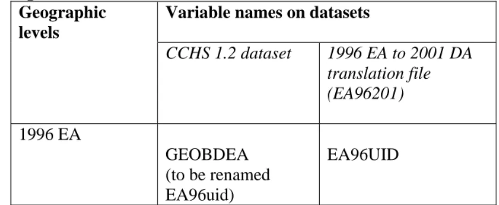
The following Figure 5 shows the datasets and variables involved in the first step of merging:
Figure 5 Geographic levels
Variable names on datasets
CCHS 1.2 dataset 1996 EA to 2001 DA translation file (EA96201) 1996 EA GEOBDEA (to be renamed EA96uid) EA96UID
2001 DA
- DA01UID
The CCHS 1.2 file is already available as a SAS dataset, but we have to run a program to create the SAS version of the translation file. Here is an example (Figure 6) of syntax for reading in the translation file, which takes you from 1996 EA to 2001 DA:
Figure 6
filename ea96201 's:\cchs\ea962o1'; data ea96201;
infile ea96201; input
@ 1 ea96uid $char8. /* 1996 enumeration area=pr(2)+fed(3)+ea(3) */ /* all with vintage 1996 census geography */ @ 10 da01uid $char8. /* 2001 dissemination area=pr(2)+cd(2)+da(4) */
/* all with vintage 2001 census geography */; run;
It is important to remember that the variable EA96uid is composed of 8 digits: PR(2), FED(3) and EA(3), all with vintage 1996 census geography. The variable DA01UID is composed of PR(2), CD(2) and DA(4), all with vintage 2001 census geography. The SAS syntax presented above does not show all the variables in the EA96201 file, but only those needed for the translation.
In order for the match merge to be successful, the CCHS dataset should have a 1996 EA code that has the same variable name and format as the 1996 EA variable in the above translation file (EA96201). All the 36,984 records of the source CCHS dataset have a match with the translation file, so we can attach a 2001 DA code to every respondent of the CCHS 1.2. Once the CCHS dataset has the 2001 DA appended to it, it can be merged to data from the 2001 DA profiles. If the contextual variables needed are at the CT level, you first also have to use the 2001 GTF correspondence files, as illustrated in Example 2 above.
In the preceding example, we described a translation scenario, which involves moving from 1996 vintage census geography to 2001 vintage census geography. Note that the process involved for a translation from a 2001 code into a 1996 code is different. It should be done using another file, as each translation file is unidirectional.8
It is also possible to conduct translations across other recent censuses. The RDC analysts can provide researchers with translation files that go back to the 1981 census. They include translations between non-contiguous censuses, such as 1986 to 1996. This should meet most of the needs for current projects. More information on the available translation files can be obtained by contacting an RDC analyst.
8. There are translation files for assigning 2001 DA from corresponding 1996 EA. However it may be more accurate to get the corresponding 1996 EA from the 2001 census block (CB), which is more precise. Researchers planning a reverse translation like this should consult an RDC analyst.
V. Merge of datasets requiring use of the Postal Code Conversion File (PCCF)--
when the survey data are lacking in geographic identifiers, and those identifiers must first be generated from postal codes present on the file
In some cases, Statistics Canada microdata files have only limited geographic identifiers available on the file. For example, the NPHS Cycle 3 dataset only contains the postal code or larger geographic groupings, such as the CMA. Those who would like to "link" the NPHS Cycle 3 with census profiles at the EA, DA or CT level must first use the PCCF or PCCF+ to convert the postal code into a full set of census geographic identifiers.
The PCCF provides a link between the postal code and standard census geographic areas. The files are updated semi-annually to reflect new and retired postal codes, and to correct errors in previous versions. For this reason, it is usually preferable to use the most current release of the PCCF or PCCF+. Alternatively, the vintage of the PCCF or PCCF+ must be at least as new as the vintage of the data file to be coded. The different vintages of the PCCF and PCCF+ are available through the Data Liberation Initiative (DLI).
Those of us who have used the PCCF to assign census geographic identifiers know that one of the biggest challenges is verifying whether or not the merge was done successfully and assessing why particular records failed to match. Using manual methods to verify the coding assigned is extremely difficult without knowing the mailing address of respondents. For this reason, analysts at Statistics Canada developed several SAS control programs and a series of reference files that can guide you through the process. The package is called PCCF+.
In PCCF+, records for postal codes which serve more than one DA--including most rural postal codes and several classes of urban postal codes--are assigned geographic codes based on a population-weighted random allocation among the possible DAs. This produces an unbiased allocation among the possible DAs. By contrast, use of the SLI (single link indicator) in the regular PCCF produces a biased allocation in such cases, incorrectly assigning all of the observations to the DA, which has the SLI, while assigning none of the observations to any of the several DAs without the SLI.
Also, PCCF+ uses various techniques to identify coding errors and suggest corrections to resolve the problem. For example: (a) if the postal code for a survey respondent is not found on the PCCF, the program uses the first three characters of the postal code (the forward sortation area, FSA) to impute or partially impute geographic coding. If the FSA is not found, it uses the first 1 or 2 characters of the postal code for partial imputation. (b) The program generates information that may help in identifying and correcting erroneous or problematic postal codes, or for finding geographic codes by other means (if possible). (c) The program identifies postal codes that are used by businesses or institutions, and specifies the building name and address in such cases. This information permits the identification of, and possible removal from the sample, of respondents who presumably reported the postal code of their place of work rather than the postal code of their place of residence. This information is also of interest to researchers who would like to remove temporary residents, such as students living in a university residence, from
the sample. (d) It deals with postal codes serving more than one EA or DA (which include most rural postal codes and several categories of urban postal codes), as well as retired postal codes. (e) It provides for translation across different vintages of census geography (or at least between the most recent and the preceding census).
For these reasons, we decided to use PCCF+ instead of the regular PCCF to assign census geographic identifiers to our NPHS Cycle 3 data. For more complete information, see the PCCF+ User’s Guide (Wilkins, 2006).
The first step is to download the latest version of PCCF+ from your local DLI website.9 The PCCF+ package includes five SAS control files, as well as a series of reference files taken from the PCCF and Weighted Conversion File. In this case, we are only interested in residential coding so we will edit the SAS program “GEORES4X” (where "X" is the letter identifying the version, such as "G" for Version 4G.).
The second step is to prepare your STC survey dataset. Presently, our most current NPHS Cycle 3 file is called “H35.sas7bdat”. It is recommended that you remove all variables from your survey dataset that are unnecessary for the merge. It is essential that you keep the postal code (in this case, SP38DPC) to enable you to merge with the PCCF, and a unique case identifier (in this case, AM58RNO) to allow you to merge back to the full microdata after you have retrieved the desired census variables. PCCF+ expects the data to be in a fixed record length (.dat) format file so we select our two linking variables and transfer the needed variables from our NPHS dataset into a fixed record length file of this format, using a PUT statement (see Figure 7).
Figure 7
FILENAME H35PCDAT 'G:\H35PC.dat';
LIBNAME NPHS 'G:\'; DATA _null_; SET NPHS.H35; FILE H35PCDAT; LENGTH ID $5 PCODE $6; ID=AM58_RNO; PCODE=SP38DPC; PUT @ 1 ID $CHAR5. @ 6 PCODE $CHAR6.; RUN;
The next step is to open GEORES4G.sas and modify the location of the data input file. You will have to show the program where to find the reference files for the PCCF+, as well as where to store the two output files produced (HLTHOUT and GEOPROB). For the purposes of this example, all of the files will be stored in G:\ (See figure 8).
9. At the time this article was written, PCCF+ 4E was the most recent version available for general use. However, Version 4G is now the current version (released January 2006).
Figure 8 /*GEORES4G.SAS */ /* *******************************************************************/ /* PCCF+ VERSION 4G WITH 2001 CENSUS GEOG */ /* *******************************************************************/ /* YOUR INPUT RECORDS EACH WITH ID+PCODE : */
FILENAME HLTHDAT 'G:\H35PC.dat';
/* THE TWO OUTPUT FILES PRODUCED: */ FILENAME HLTHOUT 'G:\H35PC.GEO'; FILENAME GEOPROB 'G:\H35PC.PRB';
FILENAME PCCFUNIQ 'G:\PCCF0510.UNIQ.CAN'; FILENAME RPO 'G:\PCCF0510.RPO.CAN'; /* GEOINS ONLY: INCLUDE RPO IN PCCFUNIQ */ FILENAME POINTDUP 'G:\POINTDUP.CAN'; FILENAME PCCFDUPS 'G:\PCCF0510.DUPS.CAN'; ..
.. ..
FILENAME QAIPPE 'G:\SESREF.QAIPE01.CAN';
As mentioned previously, each record must contain a unique case identifier (formerly AM58RNO, renamed ID) and a postal code (formerly SP38DPC, renamed PCODE). You will have to indicate where to locate these variables on your file (using an input statement). The variables were renamed ID and PCODE (see Figure 9), respectively, to reflect the naming conventions used in the SAS program. Both should be formatted as character variables.
Figure 9
/* READ IN DATA FILE WITH POSTAL CODES TO BE ASSIGNED GEOGRAPHY: */
DATA HLTHDAT0;INFILE HLTHDAT MISSOVER PAD ; ;
INPUT
@ 1 ID $CHAR5. /*UNIQUE IDENTIFIER OR REGIST NUMBER */ @ 6 PCODE $CHAR6. /* SIX DIGIT POSTAL CODE */ ;
run;
PROC SORT NODUPKEY DATA=HLTHDAT0;BY PCODE ID;
Although there are pages of SAS code to follow, no user changes to GEORES4G.sas are necessary after this point -- as long as you follow the file and variable naming conventions shown above.
You can now run the program and check the log for errors (see Figure 10). If the program ran successfully you will find a summary of automated coding results in the output window. In this example, 99.93% (49,013 of the 49,046 NPHS Cycle 3 records) were successfully assigned a full repertoire of census geographic identifiers.
---
---RECORDS PERCENT PROB MESSAGE ACTION
49046 100% TOTAL RECORDS INPUT FROM HLTHDAT (ID + PCODE)
xxxx xxx 0 ERROR: NO MATCH TO PCCF---CHECK PCODE/ADDRESS &OR CODE MANUALLY xxxx xxx 1 ERROR: LINKED TO PO GEOG--CODE MANUALLY IF RESID ADD AVAILABLE xxxx xxx 2 WARNING: NON-RESIDENTIAL--CHECK PCODE/ADDRESS (LEGITIMATE RES?) xxxx xxx 3 WARNING: BUSINESS BLDG----CHECK PCODE/ADDRESS (LEGITIMATE RES?) xxxx xxx 4 WARNING: COMMERC/INSTITU--CHECK PCODE/ADDRESS (LEGITIMATE RES?) xxxx xxx 5 WARNING: RETIRED PCODE----CHECK PCODE/ADDRESS IF OLD DMT UNKNOWN xxxx xxx 6 NOTE: MULT MATCH CSD-PCCF-DISTRIBUTED AMONG APPLIC DABLK/BLKF xxxx xxx 7 NOTE: MULT MATCH CSD-WCF--DISTRIBUTED BY POP WEIGHTS OBSERVED xxxx
------xxx 9 NO PROB (ERR,WARN,NOTE)---NO ACTION REQUIRED --- xxxx xxx NOT CODED AT ALL
xxxx xxx PARTIALLY CODED TO PR ONLY
xxxx xxx PARTIALLY CODED TO PR + (CD OR CMA)--& APPROX LAT LONG xxxx xxx PARTIALLY CODED TO PR+CD+CMA--AND APPROX LAT LONG xxxx xxx PARTIALLY CODED TO PR+CD+CMA+CSD--AND APPROX LAT LONG
49013 99.93% FULLY CODED TO PR+CD+CMA+CSD+CT+DA--AND BLK/BLKFACE LAT LONG
Following this summary table, you will receive details about the records that were not fully coded, or which are problematic for other reasons (this information is also found in the SAS dataset GEOPROB). Moving from the most serious issues to the least serious, the output file will also list the postal codes on your file that reflect non-residential addresses, business buildings, institutional addresses, and retired postal codes. You will have to make decisions based on these warnings. For example, if you are interested in the socio-demographic characteristics of a respondent’s residential neighbourhood, you may want to remove (or set to a missing value) the geographic codes of respondents who supplied a postal code relating to a business address instead of a postal code relating to a home address.
Once you have decided whether or not to remove any records from your sample (or set the geographic codes to missing values), you can merge the HLTHOUT dataset with the dataset corresponding to the full NPHS Cycle 3 microdata file. You will then be in a position to undertake a merge with the aggregate 2001 census profile data (as previously shown in Example 1).
VI. Conclusion
Appending census area-level summary data to survey or administrative data can add considerable analytical value to existing datasets. This article shows how to do that, for each of four scenarios commonly encountered by researchers. Although the examples use datasets present in Statistics Canada RDCs and show SAS syntax, the methods also apply to external datasets and can be generalized to other programming languages or statistical packages.
References
Boyle M.H. and E. L. Lipman (1998). Do Places Matter? A Multilevel Analysis of Geographic
Variations in Child Behaviour in Canada. Applied Research Branch, Strategic Policy.
Boyle, M.H. and J.D. Willms (1999). “Place effects for areas defined by administrative boundaries”. American Journal of Epidemiology, 149(6): 577-585.
Oakes, J.M. (2004). “The (mis)estimation of neighborhood effects: causal inference for a practicable social epidemiology”. Social Science and Medicine, 58: 1929-1952.
Roos, L.L, J. Magoon, S. Gupta, D. Chateau, and P.J.Veugelers (2004). “Socioeconomic determinants of mortality in two Canadian provinces: Multilevel modelling and neighborhood context”. Social Science and Medicine, 59: 1435-1447.
Ross, N.A., S. Tremblay, and K. Graham (2004). “Neighbourhood influences on health in Montréal, Canada”. Social Science and Medicine, 59: 1485-1494
Soubhi, H., P. Raina, and K. Kohen (2001). Effects of Neighbourhood, Family and Child
Behaviour on Childhood injury in Canada. Applied Research Branch Strategic Policy.
Human Resources Development Canada. W-01-1-6E.
Statistics Canada (1997). GeoRef (CD-ROM). Catalogue 92F008XCB. Geography Division. Statistics Canada (1999a). 1996 Census Dictionary – Final Edition. Catalogue no. 92-351-UIE. Statistics Canada (1999b). Information about the National Population Health Survey. Catalogue
no. 82F0068XIE.
Statistics Canada (2000). Introducing the Dissemination Area for the 2001 Census: an Update. Catalogue no. 92F0138MIE.
Statistics Canada (2002). GeoSuite 2001 (CD-ROM). Catalogue 92F0150XCB. Statistics Canada (2004a). 2001 Census Dictionary. Catalogue no. 92-378XIE.
Statistics Canada (2004b). Canadian Community Health Survey - Mental Health and Well-Being. Catalogue 82-617-XIE.
Statistics Canada (2005a). Canadian Community Health Survey - Guide. Catalogue 82M0013GPE.
Statistics Canada (2006). Postal Code Conversion File (PCCF), Reference Guide. October 2005. Catalogue no. 92F0153GIE. Geography Division.
Wilkins, R. (2006). PCCF+ Version 4G User’s Guide: Automated Geographic Coding Based on
the Statistics Postal Code Conversion Files. Health Analysis and Measurement Group,
Appendix 1.
Acronyms and simplified explanations
CB Census block. Defined for 2001 and subsequent censuses. A CB generally corresponds
to a city block (in urban areas), or to a suburban or rural area circumscribed by surrounding roads.
CA Census agglomeration. An intermediate-size statistical community consisting of
adjacent CSDs with a high degree of economic integration seen in commuting flows. Population generally in the range 10,000-99,999. CA codes are usually shown in the CMA field.
CCHS Canadian Community Health Survey (Statistics Canada, 2002).
CD Census division. A county-level census geographic unit, generally corresponding to
some sort of administrative region. A CD code is only unique within a given PR. CSD Census subdivision. A municipal-level census geography generally corresponding to a
local governmental unit. A CSD code is only unique within a given PR and CD. CMA Census metropolitan area. A large statistical community consisting of adjacent CSDs
with a high degree of economic integration seen in commuting flows. Population of at least 100,000 in the urban core at the time it was defined (but may subsequently fall below that level, yet still remain a CMA). Also a variable name for a field containing CMA and CA codes.
CT Census tract. A small-area statistical unit with a target population of about 4,000
persons (typical range from 2,500 to 8,000 persons). Only defined within CMAs and CAs with an urban core population of at least 50,000. A CT is only unique within a given CMA or CA.
DA Dissemination area. A small-area statistical unit. Beginning with the 2001 census,
replaces EA as the smallest standard unit of census geography for which aggregate census data are released. DAs have a target population of about 400 to 700 persons. A DA code is only unique within a given CD and PR.
DLI Data Liberation Initiative. The agreement between Statistics Canada and various
Canadian universities under which holdings of Statistics Canada public use files are made available for university teaching and research. (Statistics Canada website) EA Enumeration area. A small-area statistical unit for data collection and dissemination
purposes. EAs target a minimum of 125 households in rural areas to a maximum of 400 households in urban areas. However, many EAs are unpopulated. In 2001, DAs
replaced EAs as the smallest unit of standard census geography for which aggregate census data are released.
---
FED Federal electoral district. Administrative unit corresponding to the area represented by
a member of the federal parliament. A FED is only unique within a given PR. FSA Forward sortation area. A Canada Post service area corresponding to the first three
characters of a Canadian postal code.
GTF Geography Tape File. Also known as Geography Attributes File. For a given vintage of
census geography, shows each EA or DA together with all higher levels of census geography. For 1996 and 2001 census geographies, see functionally similar GeoRef and/or GeoSuite software (Statistics Canada, 1997, 2002).
NPHS National Population Health Survey (Statistics Canada, 1999).
PCCF Postal Code Conversion File (Statistics Canada, 2006). Cumulative file of all postal codes used in Canada since 1983, together with their corresponding census geography. Updated twice yearly.
PCCF+ Postal Code Conversion File Plus (Wilkins, 2006). Programs and files for intelligent geographic coding based on the PCCF. Helps identify and deal with a range of typical problems encountered. Updated twice yearly.
PR Region and province or territory. A two-digit code, with the first digit corresponding to
a region, and the second digit corresponding to a province or territory within that region.
RDC Research Data Centre. The RDC program is part of an initiative by Statistics Canada,
the Social Sciences and Humanities Research Council (SSHRC) and university
consortia to help strengthen Canada's social research capacity and to support the policy research community. RDCs provide researchers in selected sites across Canada with access, in a secure university setting, to microdata from population and household surveys. For more details, consult the RDC program Web site:
http://www.statcan.ca/english/rdc/index.htm.
Note: All levels of census geography are defined with reference to a specific census standard, which we refer to as their "vintage" (for example, the 1996 or 2001 classification). This is necessary since at any geographic level, the boundaries of a given geographic code may change across censuses, while new codes may be added or old codes removed. Postal codes also have vintages which refer to the year and month of the most recent postal codes on the corresponding PCCF release.
Source Unless other references are given within the explanation, see Statistics Canada 2001 Census Dictionary
(2004a) (Catalogue No. 92-378-XIE) and Statistics Canada 1996 Census Dictionary (1999a). (Catalogue No. 92-351-UIE)
Figure A1.1
Prior to 2001 census
EA => FED => PR => Canada
EA => CSD => CD => PR => Canada
EA => CT => CMA/CA => Canada (only within CMAs and larger CAs) 2001 and subsequent censuses
CB => FED => PR => Canada
CB => DA => CSD => CD => PR => Canada
Appendix 2
Example of SAS syntax for a merge between CCHS 2.1 data and the 2001 CT profile data, following an initial merge to append CMA+CT to the CCHS data
libname source 's:\cchs';
libname final 's:\cchs\results';
filename gtf01da 's:\cchs\gtf01da.can';
/* get the CCHS variables of interest, in the format required: */ data cchs (keep= DA01uid dhhc_age dhhc_sex genc_01 genc_07); set source.cchsmain;
DA01uid=put(GEOCDDA, 8.); Label dhhc_age = ‘Age’
dhhc_sex = ‘Sex’
genc_01 = ‘Self-perceived health’ genc_07 = ‘Self-perceived stress’
; run;
/* read in the 2001 GTF CTs corresponding to each DA: */ data gtf01da (keep=da01uid ct01uid);
infile gtf01da;
length CT01uid $ 10 zero $ 1; input
@ 1 da01uid $char8. /* pr(2)+cd(2)+da(4) */
@ 27 cma $char3. /* cma or ca incl 996-999 miz */ @ 31 ct $char6. /* census tract */
;
/* remove MIZ codes from the CMA field : */
if cma in ('996' '997' '998' '999') then CMA='000';
/* determine if the CMA/CA is census tracted or not: */ if cma in ('001' '205' '305' '310' '408' '421' '433' '442' '447' '450' '459' ''462' '505' '521' '522' '529' '532' '535' '537' '539' '541' '550' '555' '559' '562' '568' '575' '580' '590' '595' '602' '705' '725' '805' '810' '825' '830' '835' '915' '925' '932' '933' '935' '938' '970') then tracted ='1'; /* census tracted CMA or CA */ zero='0';
CT01uid=cma||zero||ct;
if CT='000.00' then tracted = '0' /* CT not defined */
else tracted = '1'; /* census tracted CMA or CA */
run;
/* get 2001 census profile data required: */
data ctprofiles (keep=CT01uid v83 v403 v407 v919 v1635); set source.ct_federal_2001_profile;
CT01uid=CTuid;
Label v83 = ‘Average number of children at home per census family’
v403 = ‘Total population by immigrant status and place of birth’ v407 = ‘Total immigrants by selected places of birth’
v919 = ‘Unemployment rate’
v1635 = ‘Median household income $’ ;
/* prepare for merge of the CCHS and GTF datasets */
/* by sorting both datasets on their common merge "by" variable: */ proc sort data=cchs; by DA01uid;
proc sort data=gtf01da; by DA01uid;
/* merge the CCHS and GTF datasets (to add CT to CCHS): */ data cchs2;
merge cchs (in=a) gtf01da (in=b); by DA01uid;
if a then output cchs2; run;
/* now prepare to merge the augmented CCHS and CT profile datasets */ /* by sorting both datasets on their common merge "by" variable */ proc sort data=cchs2; by CT01uid;
proc sort data=ctprofiles nodupkey; by CT01uid;
/* merge the augmented CCHS and CT profile datasets: */ data combined missed outside;
merge cchs2 (in=a) ctprofiles (in=b); by CT01uid;
if a and b then output combined;
else if a and not b then output missed; else if b and not a then output outside;
run;
data final.newcchs;
set combined missed; /* records with missing values for CT01uid are
retained */ run;
/* Note that all observations where TRACTED='1' are in scope */
Instructions for authors
The Information and Technical Bulletin accepts submissions for articles that address methodological or technical topics related to the datasets that are available at the Research Data Centres.
Language of material:
Manuscripts may be submitted in English or French. Accepted submissions are translated into both official languages for publication.
Length of submissions:
The maximum length of submitted articles should not exceed 20 pages, double-spaced, excluding programs and appendices. In addition to in-depth explanations of technical issues, the bulletin also accepts short (3 page) submissions that provide quick solutions to analytical problems and commentary from fellow researchers about material released previously in the bulletin.
File formats and layout of text:
Manuscripts must be submitted in Microsoft Word (.doc) and may be sent by regular mail on a disk or CD or by email.
Manuscripts must have a cover page showing the names of the authors, their primary institution of affiliation, and the contact information (telephone number, mailing address and e-mail address) of the lead author.
Manuscripts must be prepared in 12pt Times New Roman, double-spaced, with 1-inch (2.5 cm) margins.
Titles should have sentence-case capitalization (e.g., Bootstapping made easy…).
Boldface type should only be used for headings. Underlining and italics are not to be used for headings.
Footnotes and references should be single-spaced and formatted according to The Canadian
Style: A Guide to Writing and Editing.
File formats and layout of tables and charts
Tables and charts must be submitted in Microsoft Excel worksheets (.xls) or in comma-separated value (.csv) format. Each file must be clearly named table1, chart6, etc.
Tables and charts may be sent by regular mail on a disk or CD, or by e-mail.
Do not insert tables or charts into the text, but indicate their location in the text by inserting the title, followed by the filename in parentheses, e.g.,
Chart 6. Chocolate consumption by children, Canada, 2000 (chart6)
Mathematical expressions
All mathematical expressions should be set out separate from paragraph text. Equations must be numbered, with the number appearing to the right of the equation flush with the margin.
Style guide
Please follow The Canadian Style: A Guide to Writing and Editing. It is available for purchase by contacting Government of Canada Publications, Public Works and Government Services Canada.
Address for submission
Manuscripts and all correspondence relating to the contents of the Bulletin should be sent to the Editorial Committee
• by email to [email protected]
The review process
The editorial committee conducts the initial article review process. Editors may solicit past authors of the Bulletin or subject matter experts to participate in the process. The articles submitted to the Bulletin are reviewed for accuracy, consistency, and quality.
Upon completion of the initial review, the articles undergo both peer and institutional review. Peer reviews are conducted in accordance with Statistics Canada's Policy on the Review of Information Products. Institutional reviews are be conducted by members of senior management within Statistics Canada in order to ensure that the material does not compromise the Agency's guidelines of standards, or reputation for non-partisanship, objectivity and neutrality.
For more information about the review process, please contact the Editorial Committee at the address above.