Regular adjustment: theory and evidence

ISSN 1561081-0

WO R K I N G PA P E R S E R I E S

N O 6 6 9 / A U G U S T 2 0 0 6

REGULAR ADJUSTMENT

THEORY AND EVIDENCE

by Jerzy (Jurek) D. Konieczny

EUROSYSTEM INFLATION PERSISTENCE NETWORK

In 2006 all ECB publications will feature a motif taken from the €5 banknote.

W O R K I N G PA P E R S E R I E S

N O 6 6 9 / A U G U S T 2 0 0 6

This paper can be downloaded without charge from http://www.ecb.int or from the Social Science Research Network electronic library at http://ssrn.com/abstract_id=923353

REGULAR ADJUSTMENT

by Jerzy (Jurek) D. Konieczny

and Fabio Rumler

EUROSYSTEM INFLATION PERSISTENCE NETWORK

© European Central Bank, 2006 Address

Kaiserstrasse 29

60311 Frankfurt am Main, Germany Postal address

Postfach 16 03 19

60066 Frankfurt am Main, Germany Telephone +49 69 1344 0 Internet http://www.ecb.int Fax +49 69 1344 6000 Telex 411 144 ecb d All rights reserved.

Any reproduction, publication and reprint in the form of a different publication, whether printed or produced electronically, in whole or in part, is permitted only with the explicit written authorisation of the ECB or the author(s).

The views expressed in this paper do not necessarily reflect those of the European Central Bank.

The statement of purpose for the ECB Working Paper Series is available from

The Eurosystem Inflation Persistence Network

This paper reflects research conducted within the Inflation Persistence Network (IPN), a

team of Eurosystem economists undertaking joint research on inflation persistence in the

euro area and in its member countries. The research of the IPN combines theoretical and

empirical analyses using three data sources: individual consumer and producer prices;

surveys on firms’ price-setting practices; aggregated sectoral, national and area-wide

price indices. Patterns, causes and policy implications of inflation persistence are

addressed.

Since June 2005 the IPN is chaired by Frank Smets; Stephen Cecchetti (Brandeis

University), Jordi Galí (CREI, Universitat Pompeu Fabra) and Andrew Levin (Board of

Governors of the Federal Reserve System) act as external consultants and Gonzalo

Camba-Mendez as Secretary.

The refereeing process is co-ordinated by a team composed of Günter Coenen

(Chairman), Stephen Cecchetti, Silvia Fabiani, Jordi Galí, Andrew Levin, and Gonzalo

Camba-Mendez. The paper is released in order to make the results of IPN research

generally available, in preliminary form, to encourage comments and suggestions prior to

final publication. The views expressed in the paper are the author’s own and do not

necessarily reflect those of the Eurosystem.

C O N T E N T S

Abstract 4

Non-technical summary 5

1. Introduction 7

2. The model 12

2.1 Positive incidence of regular adjustments 16

2.2 Factors affecting the incidence of

regular adjustment (IRA) 20

2.3 The number problem 22

2.4 Empirical predictions under different assumptions about

policymaker heterogeneity 24

3. Empirical evidence 26

3.1 Tested hypotheses 27

3.2 Data 29

3.3 Causality 30

3.4 Result for time-regular adjustment 31

3.5 Result for state-regular adjustment 36

4. Conclusions and extensions 39

References 42

Appendix 45

Abstract

We ask why, in many circumstances and many environments, decision-makers choose to act on a time-regular basis (e.g. adjust every six weeks) or on a state-regular basis (e.g. set prices ending in a 9), even though such an approach appears suboptimal. The paper attributes regular behaviour to adjustment cost heterogeneity. We show that, given the cost heterogeneity, the likelihood of adopting regular policies depends on the shape of the benefit function: the flatter it is, the more likely, ceteris paribus, is regular adjustment. We provide sufficient conditions under which, when policymakers differ with respect to the shape of the benefit function (as in Konieczny and Skrzypacz, 2006), the frequency of adjustments across markets is negatively correlated with the incidence of regular adjustments. On the other hand, if policymakers differences are due to the level of adjustment costs (as in Dotsey, King and Wolman, 1999), then the correlation is positive.

To test the model we apply it to optimal pricing policies. We use a large Austrian data set, which consists of the direct price information collected by the statistical office and covers 80% of the CPI over eight years. We run cross-sectional tests, regressing the proportion of attractive prices and, separately, the excess proportion of price changes at the beginning of a year and at the beginning of a quarter, on various conditional frequencies of adjustment, inflation and its variability, dummies for good types, and other relevant variables. We find that the lower is, in a given market, the conditional frequency of price changes, the higher is the incidence of time- and state-regular adjustment.

JEL codes: E31, L11, E52, D01

Non-technical summary

We ask why, in many circumstances and in many environments, policy makers choose to act on a regular, rather than a state-dependent (or irregular) basis, even though such approach appears suboptimal. Perhaps the best example of regular adjustment, although it is not analyzed here, is the recent US monetary policy. Between June 2004 and May 2006, the Federal Reserve increased the federal funds rate every six weeks (16 times overall), each time by a quarter percent. Further examples of regular policies can be found in economics (price and wage adjustment, fiscal policy), management (inventory policy), engineering (machinery refurbishing), medicine (scheduling doctor’s visits) etc.

To analyze the endogenous choice between regular and irregular behaviour we develop a model in which the policymaker faces heterogeneous adjustment costs. The type of environment we consider is characterized by a continuously drifting state variable which can be adjusted using a costly control. The adjustment cost is assumed to include a lump-sum component, preventing the maintenance of the state variable continuously at the optimal level. The policymaker chooses the timing and/or the size of adjustment of the state variable so as to maximize the present value of benefits, net of adjustment costs. We consider a very simple formulation, in which the adjustment cost can take on only two values. We show that, given the heterogeneity in adjustment costs, the likelihood of adopting regular policies depends on the shape of the benefit function: the flatter it is, the more likely, ceteris paribus, is regular adjustment. Adjustment cost heterogeneity, however, is not sufficient to generate unambiguous implications of the model when policymakers are identical.

In order to obtain testable predictions, we add heterogeneity across policymakers. When policymakers differ with respect to the shape of the benefit function (as in Konieczny and Skrzypacz, 2006), the incidence of regular adjustment across policymakers is negatively correlated with the frequency of adjustments across markets and is positively correlated with the average size of adjustment. On the other hand, if policymakers differ in terms of their adjustment costs (as in Dotsey, King and Wolman, 1999), the correlation with the frequency is positive and with the adjustment size is negative.

We apply the model to nominal pricing decisions of monopolistic or monopolistically competitive firms. The state variable is the real price. It is eroded over time by inflation and can be adjusted by changing the nominal price, which is costly. We consider two types of regular adjustment: time-regular and state-regular. Time-regular adjustment is defined as changing prices at the beginning of a year or at the beginning of a quarter; state-regular adjustment is defined as setting prices at attractive levels (ending in a nine or round prices).

To test the two hypotheses on the source of differences across firms we use a large Austrian data set. It consists of direct price information collected by the Austrian Statistical Office and covers 80% of the total CPI over the period 1996-2003. We run cross-sectional tests, regressing the excess proportion of price changes at the beginning of a year and at the beginning of a quarter and, separately, the proportion of attractive prices on the conditional frequencies of adjustment, inflation and its variability, dummies for good types, and other relevant variables. We find that the lower is, in a given market, the conditional frequency of price changes, the higher is the incidence of both time- and state-regular price changes. Also, the larger is the average size of price changes, the larger is the incidence of regular price changes. These results are consistent with markets being heterogeneous with respect to the shape of the profit function, but are not consistent with markets differing with respect to the value of the adjustment costs.

Our results have implications for the effectiveness of monetary policy and the slope of the Phillips curve. Regular price adjustment makes firms’ prices less flexible and monetary policy more effective. Our model implies that the lower is the inflation rate, the greater is the incidence of regular policies and so the greater is the effect of a given monetary change on output. Furthermore, the slope of the Phillips curve may be history-dependent. Assume that switching to a regular pricing policy involves a sunk cost, for example the cost of reorganizing the pricing department. Consider a decline in the inflation rate, followed by its increase to the previous level. As the inflation rate falls, firms incur the sunk cost and switch to regular price changes. When inflation returns to the previous value, firms may continue the regular policy given the sunk cost. As a result, individual firms’ pricing policies remain inflexible and, even though inflation is the same as before, monetary policy has greater effects on output.

I. Introduction

“The [FOMC] committee agreed unanimously to lift its benchmark federal funds rate […] its 16th consecutive quarter-percentage-point increase since June 2004” The Washington Post, May 11, 2006.

In many circumstances and in many environments, decision-makers choose to act on a regular basis and, in particular, on a calendar-regular basis (e.g. once a week, on the first day of each quarter, etc.) even though such an approach appears suboptimal. Similarly, some decision-makers appear to prefer some values of the variables under their control (e.g. prices ending with a 9, interest rates which are multiples of 0.25% etc.). The focus of this paper is to analyze a simple explanation of such behaviour.

A common feature of the environments in question is their dynamic structure. The policymaker(s) maximizes a stream of benefits, which depends on the values of some state variables. Over time these values change, or deteriorate.1 _{The policymaker}

can reset the state variables but doing so involves a cost. Therefore adjustment is infrequent.

The motivation, and the focus of the paper, is the analysis of nominal price adjustment at the firm level. In this application, a firm posts the nominal price for the product(s) it sells. Due to general inflation the real price falls over time. The real price can be reset by choosing and posting a new value of the nominal price. Similar problems arise in many other environments. Therefore we begin by describing issues related to regular adjustment using examples from various potential applications.

1. Wage adjustment. Under general inflation, the purchasing power of

contractually-set wages declines over time. It can be increased in a new contract.

2. Machinery refurbishing. The capital stock deteriorates over time due to physical use or obsolescence. It is improved by refurbishing or replacing the machinery. 3. Inventory reordering. A firm holds an inventory of the product(s) it sells. The level of the inventory falls over time. It is replenished by a new delivery.

1 _{Alternatively, the current values of the state variables are constant while the optimal values drift over}

time. These problems are similar and so we will focus mostly on environments with constant optimal values.

4. Monetary policy. The Central Bank sets the interest rate appropriate for the current conditions. Over time the match between the current and the optimal value deteriorates. The interest rate can be readjusted through a decision of the Bank’s policy-making body.

5. Fiscal policy. The fiscal authority sets spending and taxation priorities in the budget. Over time the desired fiscal structure changes. It is reset in a new budget.

6. Information. Newspapers and magazines allow the public to update their

information. New events lead to its deterioration. A new issue brings the information up to date.

7. Monitoring patients. A patient’s visit allows the physician to undertake a proper course of action. Over time the health of the patient or the effectiveness of the treatment may decline. A repeat visit allows the doctor to review and adjust the treatment.

These problems are fairly common. As discussed below, they often lead to

state-contingent adjustment policies. The decision maker monitors the state variable

and applies the control whenever it has deteriorated to the threshold point. Hence the timing of adjustment does not depend solely on time and, in general, adjustments are not regular.

In practice, however, we observe many cases where controls are applied at regular moments of time. US grocery stores adjust prices on Wednesdays (Levy et al., 1997); drugstores adjust prices on Fridays (Dutta et al., 1999). Seasonal sales are held every January and July. Many firms get regular deliveries. Machinery is often refurbished on a regular basis. Labour contracts are signed for a fixed number of years. Magazines and newspapers appear with fixed frequency. Medical associations provide guidelines on the frequency of checkups and so on.

In many cases some decision-makers follow regular policies while others do not. While some firms change prices at predetermined dates, others follow state-contingent optimal pricing policies (Cecchetti,1986). Observed hazard functions of price changes in the euro area countries suggest a coexistence of state-contingent and time-regular price setting2 _{(Álvarez et al., 2005). Car firms change prices in the fall}

but offer incentives on a state-contingent basis (depending on inventory levels). Machinery is often refurbished when predetermined technical requirements are met. Some firms follow just-in-time delivery schedules, etc.

2 _{What we call time-regular policy is usually called a time-contingent policy. For clarity we avoid the}

Even when the policy is formally regular, it sometimes contains specific provisions for deviating from the schedule if needed. The interest rate may be changed between the regular meetings of the policy makers; the government may introduce a mini-budget and so on.

Furthermore, policymakers sometimes switch between regular and irregular policies. Several years ago the Bank of Canada officially moved from weekly to less frequent meetings. As implied by the above quote, in June 2004 the FED implicitly switched to regular adjustments every six weeks by 0.25%.3 Car producers have switched to just-in-time delivery policies. Most airlines nowadays use sophisticated pricing schedules, etc.

Finally, some policymakers follow different policies for different activities. Paper versions of newspapers are published regularly, but electronic versions are not.4

Some supplies may be obtained regularly while others are procured on just-in-time basis. Doctors set regular, routine visits for some patients but not for others, etc.

Understanding of regular policies is important since such policies reduce flexibility by limiting the ability of the policymaker to react to past, current and future events. It is important to note that the distinction between expected and unexpected events is not crucial here. Once the system is set up to adjust on a regular basis, the policymaker may not be able to alter the course of action for a range of both expected and unexpected changes. For example, a central bank which precommits itself to changing the interest rate on a regular basis may be unwilling to break the pattern in the face of either expected or unexpected events.

Explanations of these phenomena depend on the environment. Regular scheduling obviously reduces the cost of maintenance or of inventory delivery. Regular price adjustment may have strategic benefits (avoiding price war) or reputational benefits (easier acceptance by customers).5 Regular scheduling of monetary policy decisions helps “reducing uncertainty in the financial markets…” and “…fixed dates will allow market participants to plan and operate more efficiently.”6 Regular publishing of magazines is convenient for readers. Guidelines on the frequency of checkups simplify physicians’ decisions, etc.

3 _{In the previous 16 meetings (June 2002-May 2004) the interest rate was changed once by 0.5%, once}

by 0.25% and was unchanged 14 times; during the June 2000-May 2002 period it was changed eight times by 0.5%, three times by 0.25% and was left unchanged five times.

4 _{We are grateful to Magdalena Konieczna for suggesting this example.} 5 _{See Rotemberg (2005) and (2006) for reputation – based adjustment models.} 6 _{Bank of Canada (2000).}

Given the variety of environments and motives for adopting regular policies, in this paper we ask whether they can be accounted for with a simple, uniform framework. The model we use assumes that adjustment of the state variable is costly, but the adjustment costs are heterogeneous: they vary over time or over the values of the state variables. When the lower values of the costs occur regularly, for some policymakers regular adjustment dominates the state-contingent policy that would have been optimal if costs were homogeneous.

In order to avoid misunderstanding we want to emphasize two points. First, the adoption of this simple assumption does not mean we argue that adjustment costs are, in fact, heterogeneous in a regular manner. Second, the proposed explanation is by no means trivial.

With regard to the first issue, we treat the assumption of regularly heterogeneous adjustment costs as a simple approach to a complex problem. While applicable in some environments, this assumption is problematic in others. For example, the average unit delivery cost is likely to be lower when the firm prearranges delivery of x truckloads every y weeks rather than order inventory as needed. On the other hand, it is not clear what reduction in costs is obtained by making interest rate decisions four times a year (as the Swiss National Bank does), or by 0.25% (as the FED has been doing). Furthermore, we adopt the simplest assumption possible: we assume that the cost of adjustment is lump-sum and takes on only two values: high and low. We do not claim that this extreme simplification is realistic, but rather ask whether, with this assumption, our model can generate observed behaviour. The answer is a clear yes.

Using the assumption of heterogeneous costs may, at first thought, make our model appear trivial. As our analysis shows, however, that is not the case. We show that the results hold for an arbitrarily small difference between the high and low values of the costs. Furthermore, heterogeneous costs are neither sufficient nor necessary to explain the incidence of regular behaviour. Additional assumptions are needed to obtain testable predictions.

There are two aspects of regular nominal price adjustment we are interested in: time-regularity and state-regularity. A disproportionate proportion of price changes take place at the beginning of periods, rather than within periods. Several studies in the Inflation Persistence Network (IPN) report a high proportion of prices are held constant for a year (Álvarez et al., 2005 for Spain, Aucremanne and Dhyne, 2005 for

Belgium, Baudry et al., 2004 for France, Baumgartner et al., 2005 for Austria, Dias et al., 2005 for Portugal, Veronese et al., 2005 for Italy, Lünnemann and Mathä, 2005 for Luxembourg and Hoffmann and Kurz-Kim, 2005 for Germany). Konieczny and Skrzypacz (2005) report that, in price data collected three times a month, over a half of all changes take place in the first 10 days of a month. Similarly, several IPN studies, as well as Bergen et al. (2003) and Konieczny and Skrzypacz (2006) find that a large proportion of prices charged are attractiveprices.7

Consistent with our approach, several studies on price adjustment have recently addressed the idea of heterogeneity in adjustment costs. Levy et al. (2005) explain heterogeneity in price rigidity across holiday and non-holiday periods by variations in the cost of price adjustment. The papers by Owen and Trzepacz (2000) and by Levy et al. (2002) also contain discussions along these lines. Dotsey, King and Wolman (1999) as well as Wolman (2000) consider cross-product variation in the cost of price adjustment.

We start the paper by showing an existence result: when the costs of adjustment are lower at regular moments of time, and even when the difference is arbitrarily small, an optimizing policymaker will (except in unlikely circumstances) take advantage of the lower costs. We then show that, given the cost heterogeneity, the likelihood of adopting regular policies depends on the shape of the benefit function: the flatter it is, the more likely, ceteris paribus, is regular adjustment. In general, however, there is no clear relationship between the degree of cost heterogeneity and the incidence of regular adjustment. In order to obtain empirical predictions we add heterogeneity across policymakers. We consider two sources or differences across policymakers: the shape of the benefit function (as in Konieczny and Skrzypacz, 2006 and the size of the adjustment costs as in Dotsey, King and Wolman, 1999). We provide sufficient conditions under which, with the differences across policymakers being due to the differences in the shape of the benefit function, the frequency of adjustments across markets is negatively correlated with the incidence of regular adjustments. On the other hand, if the differences across policymakers are due to the level of adjustment costs, the correlation is positive.

7 _{Attractive prices – which sometimes are also called threshold prices or pricing points – include}

psychological prices (prices ending in 9), fractional prices (prices which are convenient to pay, such as 1.50) and round prices (defined as whole number amounts, such as 10.00).

We then apply the model to nominal price adjustment. The distinction between the time contingent, regular nominal price adjustment policies (as in Fischer,1977 and in Taylor, 1980), and state-contingent policies (as in Sheshinski and Weiss, 1977), is crucial, given their different implications for effectiveness of monetary policy (Caplin and Spulber, 1987, Caplin and Leahy, 1992).

To test the model we use a very large Austrian data set, which consists of the direct price information collected by the statistical office and covers about 80% of the CPI over eight years. We run cross-sectional tests, regressing the proportion of attractive prices and, separately, the excess proportion of price changes at the beginning of a year and at the beginning of a quarter on various conditional frequencies of adjustment, inflation and its variability, dummies for good types, and other relevant variables. We find that the lower is, in a given market, the conditional frequency of price changes, the higher is the incidence of time- and state- regular adjustment. This is consistent with markets being heterogeneous with respect to the shape of the profit function, but not consistent with markets differing with respect to the value of the menu costs.

The paper is organized as follows. The model is introduced, and the empirical predictions are derived in the next section. In section 3 we discuss the empirical evidence. Conclusions are in the last section.

II. The Model.

We consider a class of optimization problems where the value of instantaneous benefits depends on state variables that change over time. More formally, the instantaneous value of the benefits is [ ( ), ( ), ]B x t y t a , where ( )x t is a vector of state variables, ( )y t is a vector of exogenous variables and a is a vector of parameters. This formulation implies that the benefit function depends on time only indirectly.

We assume that [ ( ), ( ), ]B x t y t a is twice continuously differentiable and has a unique global maximum:

A1. For every , ( ),t y t a there exists * ( ( ), ) such that, for every ( )x y t a x t ≠ x* :

[ ( ), ( ), ] [ *, ( ), ] B x t y t a <B x y t a

Assumption A1 implies that, as long as andy a do not change, the optimal instantaneous values of the state variables are constant.

The policymaker would like to maintain the state variables continuously at the level *x or, if that is not possible, to keep them close to *x . Changes in ( )x t over time will be called the deterioration of the state variables. The policy maker can adjust

( )

x t at any time to any desired level (perhaps within some bounds), but doing so involves a discrete cost.8

The cost of adjusting the state variable, suggested by the examples above, includes the time, or the opportunity cost of the time needed to set up the decision-making process (e.g. organizing an election and counting votes, the doctor’s and the patient’s time etc.), the time needed to make and implement the decision (e.g. the time needed to set up and implement a new budget, union/employer bargaining time etc.), physical resources (e.g. new machinery, printing a new price list etc.) and non-time opportunity costs (e.g. foregone output whenever production is affected by the refurbishing process etc.).

To simplify the analysis, and in line with earlier literature (Scarf, 1959, Sheshinski and Weiss, 1977), we assume that the cost is lump-sum: independent of the size or of the frequency of adjustment. This is a reasonable assumption in some cases (monetary policy decisions, printing a new price list etc.).9

In general, the optimal solution to the optimization problems described above is state-contingent. The policymaker observes the values of the state variables and, when they reach certain thresholds, incurs the discrete cost and adjusts them to new, optimally chosen levels. State-contingent policies imply, generally, adjustment at intervals of differing length. Thresholds, as well as the new values of state variables are computed optimally and can take on any values (from an admissible range).

As discussed in the introduction, in many environments, however, we observe behaviour inconsistent with state-contingent policies: adjustment often takes place at regular intervals and some values of the state variables are chosen more often than others. We focus, therefore, on adjustment policies which we call regular policies. We distinguish between time-regular policies, which involve adjustment on a regular

8 _{In an equivalent problem, the optimal values change over time and the goal of the policymaker is to}

maintain the state variable as close as possible to the drifting optimal value, given the adjustment costs.

9 _{Adjustment costs often include, in addition, a component which depends on the size of adjustment}

basis (e.g. a firm orders new inventory every 48 days, monetary policy decision making body meets every six weeks, machinery is refurbished once every sixteen months etc.) and state-regular policies, in which newly chosen values of the state variables belong to a small subset of all possible values (e.g. inventory is ordered by a truckload, a firm selects new prices ending in a nine: 0.69, 0.79 etc.). An important subset of time-regular policies are calendar time-regular policies, which involve adjustment at calendar-related intervals (e.g. a new price list is issued once a year etc.) or where the time of applying the control is related to the calendar (e.g. sales are held at the beginning of each January and each July)

To make the analysis tractable we make several simplifying assumptions:

A2. Over the relevant range, and for any values of ( ),y t a, the effect of the vector ( )

x t on the benefit function [ ( ), ( ), ]B x t y t a can be completely summarized by a single state variable x(t).10 _{i.e. there exists B[.] such that}

[ ( ), ( ), ] [ ( ), ( ), ]

B x t y t a ≡B x t y t a and,

for every , ( ),t y t a there exists * ( ( ), )x y t a such that, for every ( )x t ≠x* :

*

'[ ( ), ( ), ] [ ( )] 0

B x t y t a ⋅ x −x t < .

where B’[.] denotes the derivative of the benefit function with respect to its first argument.

Assumption A2 means that the problem is equivalent to one in which the benefit function is a smooth, quasiconcave function of a single state variable.

The crucial assumption, which differentiates the model from earlier literature, is that the cost of adjusting x(.) may depend on time or/and on the level of x. We now consider the former case; the latter is similar and is discussed below.

To make matters as simple as possible, we divide time into periods and assume that the cost of adjustment can take on only two values: high, ch , and low, cl.

The cost is equal to the lower value for adjustment at the beginning of a period, and to the higher value for adjustments within a period. Some notation will be helpful. Let

0 1

{ , ,...}τ τ

ℑ ≡ consist of the beginnings of each period. The interval

[

)

will be called period i. Whenever the adjustment takes place at t∈ℑ, its cost is cl .

Such adjustment will be called regular adjustment and the incidence of regular

10 _{A somewhat stronger restriction is that all but one (say, the first) of the elements of the vector of state}

adjustments (IRA) will be the proportion of all adjustments which are regular, 0≤IRA≤1.

A3. The cost of adjustment is:

( ) _h ( ) ( _{l h}), _{h l}

c t = +c I t ⋅ c −c c ≥c (1)

where I(t) is an indicator function, given by:

1 for ( ) _{0 for}t

I t = _t∈ℑ_∉ℑ (2)

As the focus of the paper is regular behaviour, we further assume that periods are of the same length, i.e. τ_i's are evenly spaced over time:

0 , 1,2,....

i n n

τ τ= + ⋅τ = (3)

Obviously, the larger is the difference between the high and low values of costs, the more tempting is regular adjustment and so a large value of ch - cl makes the

problem trivial. Therefore we are careful not to make any assumptions about the size of the difference. All results hold even if the ch - cl is arbitrarily small.

In this paper we concentrate on the simple nonstochastic case. In particular: A4. The state variable x(t) is assumed to change over time at a constant rate:11

0

( ) 0

( ) ( ) t t

x t =x t ⋅e−α − (4)

Without loss of generality, we assume >0.

At the time of the first adjustment the policymaker’s goal is to pick the sequences of times of adjustment and the new values of the state variable,

0 1 1 2 2

{ ,( , ),( , ),...}

W≡ x t x t x so as to maximize the present value of the benefits:

{

}

{ } { }

11 _{As already mentioned, an equivalent problem is when the optimal value of the state variable changes}

over time and adjustments are needed to keep the actual value close to the optimal value. The second application of our theory we consider in this paper, i.e. level-regular adjustment, falls into that category: The state variable in this case is the nominal price whose optimal value (the optimal real price) drifts over time. Optimal adjustment entails resetting the price to these drifting levels or, given the heterogeneous adjustment costs across levels, to a level with lower adjustment cost. This problem can be converted into the time-dependent problem by normalizing the drifting optimal value by its trend.

where PV(W) denotes the present value of policy W, t0 is the time of the first adjustment, is the discount factor, and the first adjustment is assumed to be costless.12

The solution strategy we adopt is to start with the baseline case when y a, do not change over time and the cost of adjustment is constant and equal to its higher value, i.e. cl=ch . We then compare outcomes under heterogeneous costs with the

baseline case. Note that in both cases the value of ch is the same; they differ by the

value of cl. To set notation, the optimal policy under either case will be denoted with a

“*” and the policy under the baseline case will be denoted with a “^”.

Lemma 1.

Assume cl = ch. Let Wˆ*≡

{

}

{

}

* * *

1 2

ˆ ˆ ˆ, ,...

T = t t denote the set of the optimal adjustment times. Then _Wˆ* _{is recursive: :ˆ}* *_and

i i x x ∀ = , for all i * * * 1 ˆ_i ˆ_i ˆ t₊ = + ∆t t . Also, _Wˆ*_is unique.13 _Finally, ˆ_{( , , )ˆ} ˆ_(ˆ tˆ_{, , )} h B x y a ₋B xe− ∆α y a ₌ρc

The proof is essentially the same as in Sheshinski and Weiss (1977).

2.1. Positive Incidence of Regular Adjustments.

We now turn to showing an existence result: except in unlikely circumstances, the incidence of regular adjustments is positive: IRA>0. In other words, it is optimal for the policymaker to take advantage of the lower adjustment costs. Of course it is important that the incidence of regular adjustment is not driven by the cost saving. Proposition 1 below shows sufficient conditions under which, when cl < ch , we get

IRA>0 even if the difference ch - cl is arbitrarily small. The proof is based on the

following approximation of real numbers with rational numbers:

Lemma 2.

For every x,K>0 there exist integers N1, N2 such that N2 K and

2 1 1/

N x N⋅ − < K. Proof: see Niven (1961).

12 _{As we consider the nonstochastic case here, we omitted expectations from equation (5).}

13 _{Note that, since the optimized present value of benefits may be negative, no additional restrictions}

The lemma can be applied to the problem considered here by setting

*

ˆ /

x= ∆t τ. It implies that, if the policymaker follows a policy of adjusting once every

*

ˆ

t

∆ (which is optimal when costs of adjustment are constant), eventually an adjustment will take place arbitrarily close to the beginning of a period. Given the notation, for an arbitrary value of K, the N2th adjustment will be within 1/K of the beginning of period N1 .

Since the N2th adjustment is close to the beginning of a period, the firm needs to alter its timing just a little to take advantage of the lower beginning-of-period adjustment costs. It will do so as long as the reduction in adjustment costs exceeds the loss in benefits. Obviously, as already mentioned, we do not want the result to depend on the difference ch - cl . A sufficient condition for the results to hold regardless of the

size of ch - cl is that the slope of the benefit function be bounded; this is the motivation

for assumption (b) below:

Proposition 1.

Let *

{

}

W ≡ x t x t x denote the optimal policy, and

{

}

* * * *

0 1, , ,...2

T = t t t denote the set of the optimal adjustment times, when cl<ch.

Assume that:

(a) c(t) meets (1)-(3);

(b) the time of the first adjustment t0∈ℑ

(c) for everyy a, there existsA< ∞ such that, for every t, B x t'( ( )) <A;

Then

{

}

\{ }

T t ∩ ℑ ≠ ∅.

Proof.

Without loss of generality let the time of the first adjustment be t₀=τ₀. The proof is by contradiction. Assume that *

0

{ }

T ∩ ℑ = t . Therefore, by Lemma 1, the set of optimal adjustment times is _Tˆ*_{, with} *

0 0

ˆ

t =τ . By Lemma 2, setting A=K, there exist two positive integers N1 and N2 such that:

* 2 ˆ 1 (1/ )ln( / )h l N t∆ −Nτ< ρ c c (6a)

(

)

( )

*

ˆ

( ) ( *)

Where

{

}

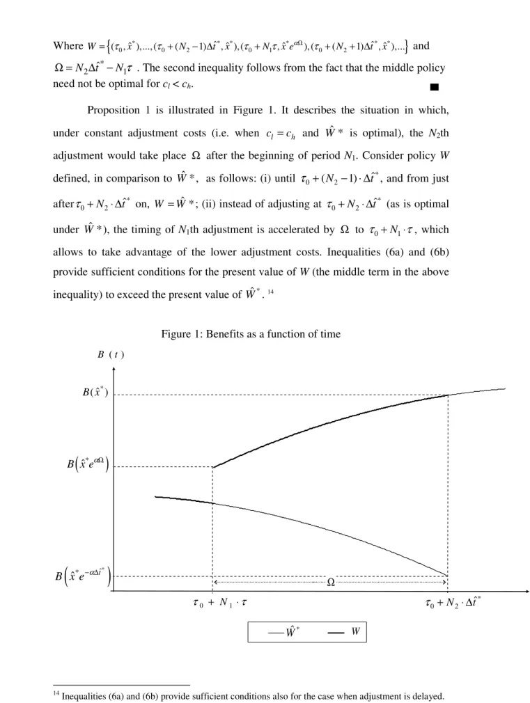
Ω = ∆ − . The second inequality follows from the fact that the middle policy need not be optimal for cl < ch.

Proposition 1 is illustrated in Figure 1. It describes the situation in which, under constant adjustment costs (i.e. when c_l =c_h and ˆW* is optimal), the N2th adjustment would take place Ω after the beginning of period N1. Consider policy W defined, in comparison to ˆW*, as follows: (i) until *

0 (N2 1) tˆ

τ + − ⋅ ∆ , and from just

after *

0 N2 tˆ

τ + ⋅∆ on, W W= ˆ *; (ii) instead of adjusting at * 0 N2 tˆ

τ + ⋅∆ (as is optimal under ˆW*), the timing of N1th adjustment is accelerated by Ω to τ₀+N₁⋅τ, which allows to take advantage of the lower adjustment costs. Inequalities (6a) and (6b) provide sufficient conditions for the present value of W (the middle term in the above inequality) to exceed the present value of _Wˆ*_. 14

Figure 1: Benefits as a function of time

14 _{Inequalities (6a) and (6b) provide sufficient conditions also for the case when adjustment is delayed.}

Ω t 0 N1 τ + ⋅τ * ˆ W W ( ) B t

(

)

(

)

Proposition 1 shows that, when the adjustment costs vary over time as postulated in A3 and the first adjustment is at the beginning of period 0 (t0∈ℑ), under

general conditions the policymaker would, sooner or later, take advantage of the lower costs of adjustment. Assumption (c) requires a discussion. If the time of the first adjustment t₀∉ℑ, it is possible that the policymaker will never take advantage of lower adjustment costs. This would be the case if, for example, ∆ =tˆ τ (i.e. when the optimal time between adjustments under constant costs is equal to the length of a period) and the difference between cl and ch is small.

In many environments, however, t0∉ℑ is an unlikely outcome. This is

because the timing of the whole sequence of subsequent adjustment times, T* \

{ }

often depends on the time of the first adjustment. For example, the timing of subsequent visits to a doctor is set relative to the initial visit, dates of subsequent delivery depend on initial delivery etc.15 _{From now on we will assume that}

0

t ∈ℑ .

By Proposition 1, at least one time of adjustment under W* coincides with the beginning of a period. To set notation, assume that the first such adjustment is the Nth adjustment, and it takes place at the end of period k. Denote such a policy as *

,

N k

W .

This means that, under * , N k W , *

{

}

It is easy to see that, for a given benefit function and adjustment costs, the optimal policy need not be unique. It is possible that *

1 ˆ k tN k τ < <τ + and PV(WN k*, ) = PV( * , 1 N k

W + ), i.e. the policymaker is indifferent between accelerating or delaying the

Nth adjustment.

The analysis of multiple equilibria in the current framework is complex. We therefore assume that, if PV( *

,

N k

W ) = PV( *

, 1

N k

W + ) then W* =WN k*, , i.e. whenever two

policies yield the same present value of benefits, the policymaker chooses the policy with later adjustments.

15 _{In environments in which the timing of adjustment is dictated by custom this need not be the case.}

For example a clothing store which opens in June may not be willing to have a sale shortly after the opening.

Proposition 2. * W is recursive:

{

}

W can be written as: *

{

}

0 0 1 1 1 1

( , ),( , ),...,(_N , _N ) , *( )_k

W τ x t x t x W τ+

− −

= , where W( )τ_k+ _is

the remainder of the optimal policy from period τk forward. Since W* is optimal and unique, by the principle of optimality W( )τ_k+ _{is the solution to the problem of}

maximizing the present value of the benefits, starting in period τk. But this problem is identical to the original problem, as can be checked by substituting, * *

i i N

t =t− .

Therefore, * 2N 2k

t =τ and _{for every such that 2 :} *

i

i N i< < N t ∉ ℑ. The proposition follows by induction.

The crucial question arising in this framework is the empirical incidence of adjustment at times inℑ, i.e. the value of IRA. By proposition 2, IRA=1/N: as the first adjustment in ℑ is the Nth adjustment and the optimal policy _W*_{is recursive, every}

1/Nth adjustment is in ℑ.16

Proposition 1 is an existence result: it shows that IRA>0 as long as ch > cl

(even if the difference ch - cl is arbitrarily small) and the benefit function is not too

steep, and subject to the discussion above. While this result is interesting, it has little empirical content, especially given the fact that the starting point of the analysis is the observation that many policies are, indeed, regular: some prices are changed at the beginning of the year, firms sometimes order a delivery of multiple truckloads etc. Therefore we now turn to the analysis of the factors which determine the incidence of regular adjustment.

2.2. Factors Affecting the Incidence of Regular Adjustment (IRA).

We address the determination of IRA in two steps. First, we consider the determinants of the incidence of regular adjustment for a single policymaker. Then we

16 _{Of particular interest is the special case of IRA=1, i.e. when N=1 *T ⊆ ℑ and the firm never pays c}

h.

Of course, T*may be a proper subset of ℑ (i.e.T*⊂ ℑ) when N=1, for example if the optimal adjustment frequency is once every two periods.

analyze empirical predictions of the model, under two alternative assumptions regarding the differences between policymakers.

Before we proceed we need to define precisely when a policymaker will deviate from the optimal policy ˆW* (i.e. the policy that she would have followed if adjustment costs were constant) to take advantage of the lower costs. We call it the

shift range:

Definition: The shift range Si = tˆ_i*−a t_i ,ˆ_i*+b_i is an interval such that the

following two conditions are met:

(a)the policymaker moves the ith adjustment from _ˆ*

i

t to someτ_j if and only if _tˆ_i*_{−ai ≤τj <t}ˆ_i* ;

(b) the policymaker moves the ith adjustment from _ˆ*

i

t to τ_j+₁, if and only

if tˆ_i*<τ_j+1≤ +tˆ_i* b_i .

In other words the policymaker moves the timing of the ith adjustment, which falls within period j, to the beginning of period j or to the beginning of period j+1 if and only if the optimal timing under constant adjustment costs falls in the shift range

Sj. Due to the fact that, by Proposition 2, W* is recursive, the index i is counted from

0

τ (or, equivalently, from the last time adjustment is at the beginning of a period). As before, we assume that if the policymaker is indifferent between accelerating or delaying adjustment, she chooses to delay it.

We now make two additional simplifying assumptions that are sufficient, although not necessary, to derive the remaining results:

A5. The benefit function is quadratic in the state variable x:

(

)

{

}

[ ( ), ( ), ] , [ ( ), ]

B x t y t a = Φ −qx + +rx s b y t a

where the functional ( , )Φ ⋅ ⋅ is an identity in its first argument.17 A6. The discount factor ρ=0.

The shift range Si determines the willingness of the policymaker to take

advantage of the lower adjustment costs. The size of Si depends on two factors: the

size of the difference ch–cl and the value of benefits foregone by departing from ˆ *W .

17 _{This formulation allows for different effects on the value of benefits of other state variables and of}

parameters, for example multiplicative _{B x t y t a[ ( ), ( ), ]= −}

(

)

(

)

[ ( ), ( ), ] b y t a

The policymaker faces a trade-off between reducing adjustment cost and the reduction in benefits brought about by not following ˆW .* The loss depends on how fast benefits decline as the time of adjustment varies. This, in turn, depends on the slope of the benefit function. A benefit function that is, at a given distance from its maximum, flat, makes the loss small and so the policymaker is willing to vary adjustment time to save on adjustment cost.

Proposition 3:

Let B1 _{and B}2 _{be two benefit functions with parameters q}1 _{and q}2 _and 1_, 2

i i

S S be

their respective shift ranges. If q1 > q2 then, for all i, 1 2

i i

b ≤b and 1 2

i i

a ≤a .

Proof.

We consider the postponement of the times of the ith adjustments tˆ_i*1 and tˆ_i*2, i.e. that

1 2

i i

b ≤b ; the proof for the acceleration of tˆ_i*1 and tˆ_i*2 is analogous. Assume i is the lowest index such that tˆi*1∈S1i . This means ti*1 is delayed until the nearest beginning

of the period, say period k1: t_i*1=τ_k1 and all prior adjustments are within periods. It is easy to show that, since the discount rate is zero by A6, the times between adjustments are all of equal length: 1

0 0

* ( ) ( / )

j k

t − =τ τ τ− ⋅ j i for all j≤i. Therefore shifting the time of the ith adjustment from t_i*1 to τ_k1involves extending all i times between adjustments by

(

)

h l

c −c is greater than i times the loss of extending adjustment time (and changing appropriately the new value of x).

Assume now that τ_k2−tˆ_i*2=τ_k1−tˆ_i*1 where τ_k2 is the first beginning of the period following tˆ_i*2. The benefit from postponing tˆ_i*2 is the saving on adjustment costs and is the same as for B1 _{but, as q}1 _{> q}2_{, the cost of the postponement is lower.}

This means that, for B2 _{, the benefit exceeds the cost. Therefore} *2 _{, 2}

k m

t =τ m k≥ ,

which implies 1 2

i i

b ≤b .

2.3. The Number Problem.

Proposition 3 shows that, for a given difference _ˆ*

i

t - τ_k and τ_k+1- _ˆ*

i

t , the flatter is the benefit function at the optimal choice, the more likely is the policymaker,

that the relationship between the second derivative of the benefit function and the incidence of regular adjustment is unambiguous. This is because the differences _ˆ*

i

t -

k

τ and τ_k+1- _ˆ*

i

t , depend on the parameters of the model in a way that depends crucially on what we call the number problem. Essentially, when c_l =c_h for any benefit function the optimal time of adjustment may happen to fall close to the beginning of a period and so a high incidence of regular adjustment may happen just by coincidence.

To provide an example, consider a given problem in which t₀ =τ₀ and _∆tˆ* _is

a well-defined, continuous function of the exogenous variables y and the parameter vectora. Assume further that, for some particular values of the exogenous variables and parameters,y₀ anda₀, we have _∆tˆ*_{=τ , i.e. under constant adjustment costs it is}

optimal for the policymaker to always adjust at the beginning of the period. In this case the policy is completely regular (IRA=1) in a neighborhood of ( , )y a_{0 0} but

IRA<1 outside this neighborhood. Since there is, in general, nothing special about( , )y a_{0 0} , the resulting policy is regular just by coincidence.

As a more specific example, assume that B=B(x,a), i.e. the benefit function depends on the state variable and one parameter. Assume that the parameter is observable and its value is positively related to_∆tˆ*_{. This is the setup considered by}

Sheshinski and Weiss (1977), where B[.] is the real profit function of a monopolist, x

is the real price and a is the inflation rate. Let adjustment costs vary as postulated here. Assume that a researcher studies six policymakers and the observable parameter

ais distributed acrosspolicymakers in such a way that their (unobservable) optimal periods of adjustment under constant cost, _ˆ*

i

t

∆ , are equal 10+i/32 months, i=15,…,20. Assume further that the difference between the high and low level of adjustment costs is so small that they never depart from ˆ *W . The incidence of regular adjustments she observes is summarized in Table 1 below:

Table 1

Monthly frequency of adjustment (%) 9.41 9.44 9.47 9.50 9.52 9.55

There is no easy way around the number problem. A potential solution is suggested by the empirical implementation below, which treats the average frequency of adjustments as an indicator of cross-policymaker heterogeneity. If the average frequency of adjustment is the variable of interest, the number problem is eliminated if the following condition on the empirical distribution of _∆tˆ* _{over time is met:}

C1. The empirical distribution of _∆tˆ*_on

{

}

i i

τ τ₋ is independent of i.

Under this condition, the probability of finding a policymaker for whom the timing of the kth adjustment, k t∆ˆ*, is within a given distance from the beginning of the period is the same for all periods.

The problem with this condition is that it is not met in practice due to truncation of the range of k_∆tˆ* _{both from below and above. The truncation from}

below is due to the fact that, under lump-sum costs, _∆tˆ*_{is bounded away from zero}

but _∆tˆ*_{is not bounded away from above from , 2 ,… The truncation from above is}

due to the fact that the limited length of the sample makes it impossible to observe policies W_{N k}*_, for which kτ exceeds the length of the sample. Therefore it is possible for results of empirical tests of the model to be dominated by the number problem. This makes it difficult to interpret rejections of the model since an empirical test of the model is a joint test of the relationship between benefit function shape and the incidence of regular adjustments as well as the fact that the number problem is “averaged out” in the data set. But the number problem is essentially a statistical issue unlikely to be affected by the considerations of the model. Hence it becomes irrelevant if the results of empirical tests are consistent with the model.

2.4. Empirical Predictions under Different Assumptions about Policymaker Heterogeneity.

The discussion above indicates that a model in which all firms are identical and their adjustment costs vary as postulated in A3 does not, in general, have unambiguous empirical implications. To obtain empirical predictions of the model, and avoid results being dominated by the number problem, heterogeneity across

policymakers is needed. Furthermore, testing should use a large data set. The second requirement rules out, for practical purposes, time-series analysis since long data series on the timing of adjustments are difficult to obtain. In the next subsection we therefore discuss empirical implications of the model under two different assumptions on cross-sectional heterogeneity across policymakers.

To obtain empirical predictions of the model we consider alternative sources of differences across policymakers: (a) with respect to the shape of the benefit function, (b) with respect to the value of adjustment costs and (c) with respect of the rate of deterioration, , of the state variable. We focus on the first two as they are tested in the next section; our data are insufficient to test model implications for the third one.

In terms of the model the benefit function heterogeneity is represented by the value of the parameter q, which determines the concavity of benefit function,. The adjustment cost heterogeneity is represented by the high value of the adjustment cost,

ch, with the difference ch –cl kept constant.

Both types of heterogeneity have been used in the modeling of optimal pricing policies under the assumption of costly price adjustment. The first type was considered by Konieczny and Skrzypacz (2006) who analyze an equilibrium optimal pricing model with costly price adjustment and consumer search for the best price. Their model, briefly described in the next section, implies that the greater is the consumer propensity to search for the best price in a given market, the greater is the value of the parameter q. The second type of heterogeneity was considered by Dotsey, King and Wolman (1999) who develop a tractable framework incorporating costly price adjustment into a general equilibrium model. In their approach firms differ with respect to their adjustment costs.

As shown below, the two assumptions produce opposite results and so an empirical study we propose can, potentially, discriminate between them under the joint hypothesis that adjustment costs vary as postulated in our model.

Proposition 4.

Consider an environment with many policymakers whose benefit functions are as in A5, and whose adjustment costs vary over time (or over states) as postulated in A3. For all policymakers let ˆ* (0, ]t ∈ τ_n , n≥1 and assume that

the condition C1 is met for all i≤n. Assume further that policymakers are identical except for one source of heterogeneity across policymakers:

(a) If the differences across policymakers are due to differences in the value of

q, then the lower is q, the less frequent is adjustment and the higher is the incidence of regular adjustment.

(b) If the differences across policymakers are due to differences in the value of

ch and cl (so that ch - cl is the same across policymakers) then the higher ch ,

the less frequent is adjustment and the lower is the incidence of regular adjustment.18

(c) If the differences across policymakers are due to differences in the value of

α, then the lower is the value of α, the less frequent is adjustment and the higher is the incidence of regular adjustment.

Proof:

The effect on the frequency of adjustment in 4(a) follows directly from the Lemma (Konieczny and Skrzypacz (2006)); in 4(b) it follows directly from Sheshinski and Weiss (1977), section 5 and in 4(c) it follows directly from Proposition 2 in Sheshinski and Weiss (1977) since the quadratic benefit function meets their condition (M).19 The effects on IRA follow directly from proposition 3.

III. Empirical Evidence.

We test the model by analyzing optimal pricing policies at the firm level. In the pricing application the benefit function B[.,.,.] is the profit function of a monopolistic, or monopolistically competitive firm which produces a single product. Under general inflation at the rate , its real price falls over time. To reset it the firm changes its nominal price, which involves paying a lump-sum menu cost.

18 _{To avoid confusion note that in (b) there are two sources of heterogeneity in adjustment costs. The}

first source is heterogeneity in the size of adjustment costs over time (or over states), as postulated in A3. It is the same for all policymakers. The second source is heterogeneity across policymakers. In (a) and (c) the differences in adjustment costs are due to the first source only.

19 _{As long as xˆ * exp(− ∆α tˆ*)>x* / 2, where x* is the benefit-maximizing value of x in the absence of}

3.1. Tested Hypotheses.

The data allow us to analyze the incidence of both time-regular and state-regular policies. We define a time-state-regular policy as price adjustment at the beginning of the year, and, separately, as price adjustment at the beginning of a quarter. We will refer to such policies as seasonal price setting. State-regular policies involve choosing

attractive prices: prices that end in a nine or round prices. The definition (values) of attractive prices is given in the Appendix.

Our data set, which we describe below, does not allow for a direct test of Proposition 4(c) as the variation in the inflation rate in the data is small. Therefore we concentrate on the differences across firms in the shape of the profit function and in the values of adjustment costs.

Our H0 hypothesis, implied by Proposition 4(a), is that the adjustment costs

vary as postulated and that the differences across policymakers are due to heterogeneity in the shape of the profit function, as in Konieczny and Skrzypacz (2006). The alternative, implied by Proposition 4(b), is that the differences are due to heterogeneity in the level of price adjustment costs, as in Dotsey, King and Wolman (1999).

The data set used to test the model is extensive and the variation in the endogenous variable is large. Therefore we would treat an insignificant estimated coefficient on the adjustment frequency as a rejection of the model, notwithstanding the number problem. If the coefficient is negative and significant, we treat it as support for the joint hypothesis that menu costs vary as postulated and heterogeneity across markets is due to differences in the shape (curvature) of the profit function. If it is positive and significant, we treat it as support for the joint hypothesis that menu costs vary as postulated and heterogeneity across markets is due to differences in the size of the menu costs.

Since neither the curvature nor the value of adjustment costs is observable in our data, a direct test of the model is not possible. However, an indirect test of the model can be performed with another variable acting as an instrument for the unobservable variable. In view of Proposition 4, we treat the adjustment frequency as the instrument.

Before we turn to the data, we now briefly describe the two underlying models of policymaker heterogeneity.

Konieczny and Skrzypacz (2006) analyze a model, based on Bénabou (1992), in which firms face nominal adjustment costs and consumer search for the best price. They consider a market for a single good which is supplied by a continuum of firms, each with the same marginal cost MC. Firms set nominal prices so as to maximize the average value of real profits per unit of time. Nominal prices are eroded by constant inflation at the rate . As price adjustment is costly, nominal prices are changed infrequently. In the absence of perfect synchronization prices differ across firms.

Each period a new cohort of v consumers per firm arrives in the market. Each consumer buys 0 or k units of the good and exits the market. Consumers search for the best price. They are heterogeneous in terms of their adjustment costs c, which is distributed uniformly over the range [0,C] in each cohort. Heterogeneity across markets is due to differences in the values of the parameters k and C, which determine the propensity to search for the best price, and the density of customers, v.

The model is directly applicable to our framework. Konieczny and Skrzypacz (2006) show that the profit function is, using our notation20 B(x) = - qx2+rx+s. The parameter q, which is crucial in our study since it determines the concavity of the benefit function, is a simple function of k, C and v: q=vk2_{/C. More active search for}

the best price, due to a large amount spent on the good (large k) or low search costs (represented by a low maximum value C), or a large number of customers (large v), lead to more concave profit functions.

Dotsey, King and Wolman (1999) develop a general equilibrium framework for the dynamic analysis of the effects of various macro disturbances in the presence of price adjustment costs. In their model both firms and consumers are long lived. Consumers have Dixit-Stiglitz preferences for variety and so firms are monopolistically competitive. Heterogeneity is due to differences in the value of adjustment costs: firms draw them independently over time from a continuous distribution.

The model is a general equilibrium one, but for fixed values of exogenous parameters it can be interpreted as a multi-market model. As the Dixit-Stiglitz preferences imply constant-elasticity demand, the profit functions are not quadratic. The results of our model hold when the profit functions can be approximated with a quadratic, i.e. for low values of adjustment costs and/or low inflation. While the

20 _{Here x is the real price, q=vk}2_{/C, r=q(C/k+E(x)+MC), s= MC [C/k+E(x)] and E(x) is the average}