Semantic Segmentation For Free Drive-able Space Estimation

(1)

Semantic Segmentation For Free

Drive-able Space Estimation

Master Thesis

Submitted in Fulfillment of the

Requirements for the Academic Degree

M.Sc. Automotive Software Engineering

Dept. of Computer Science

Chair of Computer Engineering

Submitted by: Eric Gallagher Student ID: 426158

Date: 12.08.2019

Supervising tutor: Prof. Dr. W. Hardt Supervising tutor: Mr Shadi Saleh M.Sc.

(2)

Acknowledgments

I would like to express my gratitude to Mr Shadi Saleh for his continued support during my thesis. His willingness to give generously of his time has been very much appreciated. He has actively encouraged me to achieve the best possible result. He has provided much useful constructive critique and patient guidance. Without his support this thesis could not have been completed.

(3)

Abstract

Autonomous Vehicles need precise information as to the Drive-able space in order to be able to safely navigate. In recent years deep learning and Semantic

Segmentation have attracted intense research. It is a highly advancing and rapidly evolving field that continues to provide excellent results. Research has shown that deep learning is emerging as a powerful tool in many applications. The aim of this study is to develop a deep learning system to estimate the Free Drive-able space. Building on the state of the art deep learning techniques, semantic segmentation will be used to replace the need for highly accurate maps, that are expensive to license. Free Drive-able space is defined as the drive-able space on the correct side of the road, that can be reached without a collision with another road user or pedestrian. A state of the art deep network will be trained with a custom data-set in order to learn complex driving decisions. Motivated by good results, further deep learning techniques will be applied to measure distance from monocular images. The findings demonstrate the power of deep learning techniques in complex driving decisions. The results also indicate the economic and technical feasibility of semantic segmentation over expensive high definition maps.

Keywords: Deep Learning, Semantic Segmentation, Monocular Depth Estimation

(4)

List of Figures

2.1 Types of occupancy Grids . . . 18

2.2 Segmentation using Super Pixels . . . 20

2.3 Example of Lane Segmentation[14] . . . 26

2.4 Bicycle Lane Segmented as Ego Lane [14] . . . 27

2.5 Overview of literature review . . . 27

3.1 Biological Neuron . . . 30

3.2 Mathematical Model . . . 30

3.3 Multi Layer Preceptron Networks[15] . . . 31

3.4 Gradient Descent . . . 34

3.5 Convolution Operation . . . 35

3.6 Feature Maps . . . 35

3.7 Output Height Dimensions . . . 36

3.8 Output Width Dimensions . . . 36

3.9 Original Inception Module . . . 40

3.10 Inception Module with Factorized Convolutions . . . 40

3.11 Equivalent module to Original Inception . . . 41

3.12 Extreme Version of Original Inception . . . 42

3.13 Shift and Stitch . . . 43

3.14 Altrois Convolution . . . 44

3.15 Fully Convolutional Network Architecture . . . 45

3.16 Normal Convolutions . . . 50

3.17 Point wise Convolutions . . . 50

3.18 Depth wise Convolutions . . . 51

3.19 Deep Lab V3+ Architecture . . . 52

3.20 Network Based Transfer Learning . . . 54

(7)

LIST OF FIGURES

3.22 Masking Static Pixels . . . 57

3.23 Relative Squared Error . . . 58

3.24 Relative Absolute Error . . . 59

3.25 Root Mean Squared Error . . . 59

4.1 Segmentation Data Flow Diagram . . . 60

4.2 Tensorflow Overview . . . 61

4.3 One clock cycle per instruction . . . 63

4.4 Three instructions per clock cycle . . . 63

4.5 Example of Original Image and Labeled Image . . . 65

4.6 Add Images . . . 68

4.7 Pixels with out of range colors . . . 69

4.8 List of labels . . . 70

4.9 Screen shot of mIOU . . . 75

4.10 Distance Estimation Outline . . . 80

4.11 Illustration of Pixel based measurement. . . 81

4.12 Test Image for Pixel Based Measurement . . . 82

4.13 Depth Measurement Original . . . 84

4.14 Merging Depth Segmentation and Original Images . . . 85

4.15 Depth Measurement With Ground Truth . . . 87

4.18 Depth Measurement . . . 88

5.1 mIOU Illustration . . . 91

5.2 Mean Intersection over Union . . . 91

5.3 Segmentation of opposite lane and ego lane . . . 92

5.4 Segmentation of opposite lane and ego lane . . . 92

5.5 Segmentation in Dark Conditions . . . 93

5.6 Segmentation on Unmarked Roads . . . 93

5.7 Adverse Conditions . . . 94

5.8 Obscured View . . . 94

(8)

LIST OF FIGURES

5.10 Dark Conditions Conditions . . . 95

5.11 Strong Glare . . . 96

5.12 Construction Sites . . . 96

(9)

List of Tables

2.1 Accuracy Results . . . 23

2.2 Accuracy Results Lane Segmentation . . . 26

4.1 Results from distance measurement . . . 86

(10)

List of Abbreviations

CNN Convolutional Neural Network

FCN Fully Connected Neural Network

DNN Deep Neural Network

DCNN Deep Convolutional Neural Network

SVN Support Vector Machine

mIOU Mean Intersection Over Union

GPU Graphics Processor Unit

ADAS Advanced Driver Assistance Systems

BDD Berkeley Deep Drive

SGM Semi Global Matching

SGD Stochastic Gradient Descent

ASPP Atrous Spatial Pyramid Pooling

CRF Conditional Random Field

VGG Visual Graphics Group

API Application Programming Interface

(11)

1 Introduction

Over Recent years interest in ADAS systems has gained significant interest in research and industry. As driver error is the leading cause of road traffic accidents and fatalities, ADAS systems have been used to improve the safety of vehicles. Free Drive-able space estimation is the back bone of many ADAS and highly automated driving. If it is possible to solve this problem in a cost efficient and robust manner, a significant step forward in highly automated driving will have been taken.

1.1 Free Drive-able Space Estimation

Free Drive-able Space is the space on the correct side of the road that can be reached by an autonomous car without colliding with another car, pedestrian or other object.

Identifying

Free Drive-able space involves two major challenges namely identifying and estimating. Identifying objects involves training a deep network to learn to recognize parts of the roads such as correct lane and oncoming lane. Next of all the network must learn to recognize obstacles in the path of the correct lane and adjust the drive-able space accordingly.

Estimating

Identifying objects is of paramount importance however estimating the distance to these objects must also be given due consideration.

As the research of my supervisor Mr. Shadi Saleh focuses on depth information from monocular images based on Convolutional Neural Networks and minimal data. I will use a pre trained CNN to estimate depth information. I will also validate the measurements with a Computer Vision measurement technique.

(12)

1 Introduction

Results from this technique demonstrate that state of the art methods can provide plausible results even with minimal data.

However, as this thesis is primary concerned with Semantic Segmentation, depth estimation will be considered briefly. It is by no means a complete study.

1.2 Problem Statement

The inhibiting factors of highly automated driving are economic factors and technological factors.

LiDAR and RADAR sensors are 75k plus and their performance degrades in rain fog and snow. These are also the time when advanced driver assistance systems are most needed. These sensors also do not detect the density of objects and have limited range. An autonomous vehicle needs expensive GPS sensors and also relies on high definition maps which are expensive to license. The costs and

disadvantages of these sensors are an inhibiting factor in highly automated driving. Vision based sensors on the other hand are a low cost sensor. Vision based sensors are capable of capturing rich semantic information. They can also provide long range distance detection. Deep Learning is a rapidly advancing field that continues to achieve excellent results. Semantic Segmentation has emerged as powerful tool, it is capable of providing pixel wise precision accuracy of images. Furthermore the generalization power of Deep learning has shown that it is capable of dealing with out of the ordinary situations. Deep learning has shown significant progress in bridging the economic and technological gap in highly automated driving.

1.3 Motivation and Objectives

The aim of this work is to use effective deep learning methods in order to solve the problem of free-drivable space estimation, as this is a complex driving decision, it will need to be broken down into three research objectives.

The first research objective is to segment the correct lane and opposite lane. This is the most fundamental objective to develop a model that can generically identify free drive-able space. As deep learning tries to find interconnections between

(13)

1 Introduction

objects, the network needs to learn to identify the road initially, from there more precise information can be learned such as opposite lane and correct lane.

The Second Research Objective is identification obstacles in the correct driving lane, this necessary to identify collision free drive-able space. Obstacles such as other road users and pedestrians need to be identified, and learned by the network. Furthermore they need to be reflected in the free drive-able space identified.

The third research objective, is to estimate the space in meters that has been identified as free drive-able space.

1.4 Semantic Segmentation

Semantic Segmentation

Semantic Segmentation involves assigning a label to every pixel in the image. It aims to provide complete image understanding, more specifically understand the image at pixel level. It is a long standing research problem in computer vision. Semantic Segmentation, is emerging as a powerful tool in computer vision and has made major advances in recent years especially in autonomous driving and medical imaging.

Deep Learning methods have attracted intense research since 2012 when

Krizhevsky et al made a mayor breakthrough in image classification [11]. Since then, Deep Learning has significantly boosted segmentation model’s generalization power and accuracy. It has attracted intensive research with a large amount of papers being frequently published at a high complexity. Semantic Segmentation has been successfully applied in many industries such as automotive medical imaging and area photography. Similarly industry has raced to develop new frameworks for increased Segmentation accuracy. These Networks have become increasingly more accurate and continue to achieve excellent results, this not only due to increased amounts of data and more powerful GPUs, but the research and development interest in Segmentation.

(14)

1 Introduction

1.5 Thesis Structure

In order to provide a solution to the Objectives, this study is as structured as follows. As Deep Learning is a broad and highly advancing field, a Literature review is used in order to identify a very specific area to concentrate on. Next as Deep Learning is a complex task a through technological background will be given. This will result in identification of a state of the art network namely Deeplab V3+. Data Preparation will be given due consideration, as good deep learning results are highly data dependent. A rarely used data set namely, Berkeley Deep Drive will be prepared as the data set. The labels will be combined to achieve a more accurate data set for free space estimation. Deeplab V3+ will be trained to segment the free drive-able space. Distance estimation will be briefly considered. Finally the segmentation results will be evaluated.

(15)

2 Literature Review

Literature Review

This chapter will give an overview of literature relating to semantic segmentation for free drive-able space estimation. The chapter is structured as follows, computer vision techniques will be considered first, next machine learning and finally deep learning. The main focus will be on deep learning. computer vision and machine learning techniques should not be disregarded as they can complement deep learning techniques, and also help to solve the inherent data dependency problem of deep learning.

2.1 Computer Vision

Computer Vision Techniques

The Literature Review will begin with a review of research areas done by the Department of Computer Engineering. Self Organizing Systems is a main research topic at this department. Distributed embedded self organizing systems aim to be independent entities capable of solving specific tasks and exchanging information. As they are self organizing, there is no single point of failure. Furthermore they are economically and computationally cost efficient. Research papers from the project Automated Power Line Inspection (APOLI) will be considered first. Next a Stereo Vision approach to Map a 3D point cloud will be considered.

Subsequently two more papers will be dealt with, these use a mixture of stereo vision and grid based processing to estimate the free drive-able space.

In [25] the authors set out to develop a computer vision algorithm to detect damaged insulators. The system has multiple advantages. It reduces the time, costs and of inspecting power lines. Furthermore it also reduces cut out times of

(16)

2 Literature Review

the electricity supply. It improves the safety and accuracy of fault detection. In order to solve this problem the authors used a vision based system. The first step in processing is gray scaling, next a ROI is used to identify the parts of the insulator where damage occurred. Next a blob detector is used to detect burn marks resulting from damage. Size, color and shape are the parameters used to model the blob. Finally the blobs are weighted by their probabilities based on their location in the ROI.

In this paper the authors implemented a fault detector for power insulators. It is a reliable embedded system, with a low economic and computational cost. The overall accuracy result was 80.43 percent.

In [4] the author developed a system to detect high voltage power lines, along with their direction without any camera position information. Drones are highly useful as automated inspection instruments. They can reduce the risk and costs of

inspection and also allow uninterrupted supply of power. Due to the interference of high power lines on GPS signals, vision based sensors are a viable alternative. The algorithm uses edge detection and line detection to identify power lines. In order to improve the accuracy a clustering technique is used. To detect the direction of the power lines, the authors defined two scenarios. Firstly if the clustering points intersect outside of the frame, line clustering is used. Secondly if the points intersect inside of the frame, K-means clustering is used. Finally a ROI was defined to determine the direction of the power lines based on fitting a triangle to clustering points. In this work the authors solved the problem of accurate High Voltage Power Line detection, and detection of the direction of the power lines. In [20] the authors find an alternative to RADAR and LiDAR. The two

technologies are financially and computationally expensive and also fail in adverse weather conditions. They set out to develop a low cost, stereo camera based solution, that can provide a highly accurate 3D point cloud.

In solving the problem of spatial environment mapping, the authors define three maps they are namely a Height map, a Confidence map and an Occlusion map. The height map will be considered first.

Height Map

The Height Map results from projecting the 3D point cloud over a 2D Map. More specifically it contains cells that display the height of objects present in each cell.

(17)

2 Literature Review

Colors are used to quantitative the height of points in each cell. The Height map consists of global height and local height. Local height is a 3D point cloud

mapping, and changes as the Region of interest changes. Global height is a 2D static map and it is updated if the local map falls within region of this map.

Confidence Map

The purpose of the confidence map is two fold. Firstly it is used to remove outliers and secondly it is used to threshold a function to see if the cell is occluded or not.

Occlusion Map

The occlusion map is used to remove inaccurate sensor measurements. Cells are assigned the status of free, border or occluded. Finally remove cells that are occluded by cells in the same cluster, in order to calculate object boundaries.

Methodology

In order to find occluded cells the local height map is used. Points are clustered based on euclidean distance. A center is assigned to the cluster. The center is adjusted as new cells are added. The whole cluster is thresholded based on the number of cells. A boundary box is defined for the cluster and the cluster center is redefined. Finally it is important to differentiate between boundary cells and border cells. Boundary cells are cells that contain the edges of an object whereas border cells are boundary cells with the closest distance to the sensor.

In this work [20] created a low cost 3D point cloud, that is economical in terms of cost and computational resource requirements. It is a reliable measurement sensor, that also defines a useful structure to fuse sensor data. Sensor fusion is attracting intensive research at present. It is of paramount importance that this data can be fused and represented it a reliable and robust manor. Furthermore this paper allows for future scope in deep learning techniques such a monocular vision to further improve its performance.

The sixtel world [2] is a compact and medium level representation of the world. Stixel stands for Stick Pixel It is a simplified model of the world using a ground plane and a set of vertical sticks on the ground representing obstacles. In order to solve the problem the authors used a Disparity Map and Occupancy Grids.

(18)

2 Literature Review Disparity Map

Depth in an image can be calculated by Stereo Pairs. Depth and disparity are inversely proportional. A Stereo Matching Algorithm is used to find matching points. The distance between these points is proportional to the depth in the image. The algorithm searches the Y coordinate of each image to find

corresponding points.

A large distance between matching points means that the object is close to the camera, a small distance means the the object is far away from the camera. Occlusion means that the view to a point is obstructed. To solve this the value of last pixel is given. Semi Global Matching algorithm, is regarded by [2] as the optimal algorithm in Stereo matching.

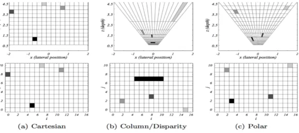
Occupancy Grids

Occupancy grids are a 2D array which models the real world. It is projected onto the ground place. Each cell of the array contains a lateral component and depth component . Each grid of the occupancy model can calculate the probability of the grid being free or occupied. Pixel values are compared, to neighboring grids to check if the grid is occupied. There are three types of occupancy grids as per Fig[2.1]

(19)

2 Literature Review Graph Based Segmentation

Graph Based Segmentation is a computer vision technique used to segment images. It works on the following principals. Each Pixel is a Node. Each node is linked to other Nodes via Edges. Edges are weighted by similarity to other pixels. Neighboring Pixels should have the same label unless they have very different intensities, edges are cut in order to define boundaries between shapes. Labels are assigned to objects.

In very basic terms sixtels are defined as any object that is not flat in an image, it uses stereo vision techniques to estimate depth. [2] Applied a Stereo disparity map to an occupancy grid, to calculate free drive-able space. They then segmented the foreground and Background, using graph based segmentation. This resulted in a height map. The height map allowed the authors to identify the base and height of objects, with this information 3D Stixels can be fitted to objects.

In [19] the authors defined two confidence maps one for road and one for obstacle. Both of these maps were combined in a weighted accumulation manner. The V disparity map is a sliding window that measures the vertical disparity in the image. An overview of the algorithm is as follows, calculate the V disparity map, use the sobel operator to calculate multiple sub V disparity maps, find the

maximum intensity pixel for each column. Finally apply ground correlation by use of the Hough Transform.

The advantages are that the algorithm works on a non flat plane, with varying latitudinal slopes. It doesn’t fail in complex scenes and can detect multiple roads, overall it is a robust method. It can work on a wide variety of terrains and

achieved an F1 Score 97.46 percent. Unfortunately it is not illumination invariant and does not detect road boundaries, it also does not react to road markings.

2.2 Machine Learning

In [27], they used a mixture of computer vision techniques and machine learning, In terms of Computer vision they used graph based segmentation, in terms of machine learning the used a support vector machine SVM. In order to use graph

(20)

2 Literature Review

based segmentation a function has to be defined. Color, homography and geometric features were used to exploit information that is used to define an energy function for a graph. The main contribution of this paper is to show that a stereo pairs in not necessary in calculating the free space. Calculating the free space in stereo pairs is a straight forward problem. Obstacles can easily be identified when depth information is available. However significant issues arise in monocular images as lane markings provide strong gradients however they are not obstacles. Monocular approaches generally rely on edges or geometry to segment the ground plane. This paper also uses edges, color and and homography as an energy function to segment the ground plane however a SVM was used to learn the optimal parameters, this SVM feeds a 1D Markov Random field. This type of data structure is a graph, where every node represents a column in the image and its label represents a position in the ground plane that segments the free space from obstacles. The proposed method offers numerous advantages. A single low cost camera is used. The task is implemented the challenging KITTI data set, it offers fast and exact segmentation of 4000 frames in real time at only 0.1 second per frame. Furthermore it achieves an F1 score of 96.35 percent. The technique however relies on previous frames to calculate the next frame. It fails in scenes with poor road markings and confuses road and pavement.

In [22] the authors used super pixels to segment free space. Initially a Stereo pair image was used to form a disparity map, using SGM Semi Global Matching. The Color image was segmented into super pixels, using the plane normal vector. Next the Disparity map was combined with super pixels for form the final result. An overview of the algorithm is given in Fig[2.2]

(21)

2 Literature Review Advantages

This algorithm is illumination invariant, it does not rely on primitives such as edges, colors, intensity or shape. It works in a variety of situations and is not limited to well maintained roads. Overall it achieved a detection rate of 97.7 percent, a detection accuracy of 96.5 percent, and an effectiveness rate of 97.1 percent. It does not require a GPU rather it can run on an 3.4GHz processor with 8 GB RAM. It can process a single image in 0.4 seconds, meaning only 2.5 frames per second.

Disadvantages

It assumes that the center of the image is free space which may not be the situation in urban environments. It requires manual labeling of 100 ground truth images.

2.3 Deep Learning

Deep Learning Methods

In [10] Is a deep learning and computer vision technique. A general overview of the algorithm is as follows. Segmentation is done by a disparity map and graph cuts. The output is then used to train a weak classifier. If the graph cut segmentation result, and the Fully Convolutional Network segmentation results match than the result is final, otherwise the FCN is retrained.

It’s advantages are that it is a Self Supervised learning technique. It does not require off-line training, also it does not require a large amount of data. It works on off-road terrain with a variation in topographical information. Furthermore the Ground Plane does not have to be largest Plane. The system was tested in easy, moderate and difficult terrain. Overall it achieved a average F1 Score 93 percent. Unfortunately it is 6 Times Slower than an FCN and also vulnerable to over fitting. Either more validation should be done on the network or the FCN should only be retrained when there is a significant difference between the Graph cut segmentation and the FCN segmentation.

In [17] the authors used the following method to solve the given problem and it is as follows, firstly SGM was used. Next Super pixels were used as an average measurement of depth. The method relies on a Stereo Camera as its main sensor,

(22)

2 Literature Review

but also uses radar sensors. The area in front of the car is divided into 70 segments, and the distance to each segment is calculated.

As a significant amount of data over 4 million segments were produced, a

semi-novel validation method was used. The camera based free space estimation was validated with laser measurements. While the proposed method does offer semi-novel validation strategies and could be used in deep learning, the system suffers from low illumination, rain and glare.

In [3] the authors developed a Fully Convolutional Network. An FCN is

Remodeled from CNN Architecture. All fully connected layers are replaced with deconvolutional layers. It is better suited to segmentation tasks as down sampling identifies features whereas up sampling identifies where. Image segmentation involves separating images into specific groups of similar pixels and labeling The key advantage of an FCN is that there is no loss of spatial context

Advantages

The Seg Net architecture overcomes blocky segmentation due to max pooling. Decoders map output from one segmentation prediction to the next up-sampled prediction to provide for more smooth and accurate predictions.

The FCN is illumination Invariant. It is also capable of detecting small objects such as polls. The network was trained from scratch and achieved good results with only 2 forward and backwards passes over the whole dataset. Overall the FCN achieved an accuracy score of 84 percent over 12 classes

However the Network has some disadvantages, cars misclassified as pavement, furthermore it requires a large amount of data and resources to achieve good results.

In [21] the authors used an FCN and trained it in a self supervised manner. He set out to achieve similar results to manually labeled data. His method used weakly supervised labels, generated by a disparity map and the sixtel world. Like other researchers in the field he outlines two problems one the trade-off of weakly

supervised learning versus fully supervised learning. The second problem is that of finding a way to manually label data. In attempting to find an algorithm that can manually generate labels one finds the exact problem that needs to be solved [21]. The network employed was a CN24. A semi supervised technique used was the

(23)

2 Literature Review

sixel world as highlighted earlier. The sixtel world map will provide weak labels for the FCN to train on. The solution to the problem used stereo vision and the sixtel world. The sixtel world will generate weak labels that the FCN can train on. Although the Sixtel representation may contain some errors, the generalization of the FCN will average out the errors.

Data Set

The training set consists of 188 frames of manually labeled data with 10 preceding frames. The test set consists of 265 hand annotated frames in every 10 frames. The algorithm achieved the following accuracy results as Per Table[2.1]

Accuracy Trained Offline Trained Online From Scratch Fine Tuned

F1 Max 0.87 0.91 0.92

Average Precision 0.97 0.98 0.98

Table 2.1: Accuracy Results

Disadvantages

An issue of the method is the it does not provide good segmentation results. Road and also footpath are segmented as the same. There is no distance estimation also. Even though Stereo vision has been employed along with Stixel world

representation. Both of which can easily give the result of depth. In designing a system one should get the most information from the data and processing. Using distance estimation methods solely as self supervised training is disadvantageous.

Advantages

It is a self supervised technique, and reduces the need for large manually annotated datasets. the model is fine tuned for different task specific situations such as urban, extra urban and suburban. The author proposes a method to select many different classifiers and select the one that is most relevant for the specific situation. It is useful that the author differentiates models for urban and extra urban scenarios. It allows greater accuracy, as different scenarios would prose different challenges. It does not presume that the bottom of the image is free space which many other algorithms rely upon. This is a false assumption especially in urban traffic.

(24)

2 Literature Review

In [18], the author used 30 hours of data overall it consisted of 13,000 training images 1,300 testing images and 1,300 validation images. The author uses two labeled data sets one is a lane data set and another is a vehicle data set. More specifically the data set consisted of annotated lane markings within 80 meters. Labels are included regardless if they are occluded or not. Labeled markings were obtained form accurate LiDAR point cloud. Lane markings were extracted

manually then reviewed by humans. The author defines free space as the distance between two labels that does not have a vehicle in it. The final data-set contains 13,000 training images,1,300 validation images, and 1,300 test images.

Technical approach

Modified Google Le Net

This is the same as Goggle Le Net up to the average pooling layer. As the network was trained for image classification. The average pooling layer would result in a loss of spatial information. Localization uses a modified over feat architecture. A one by one convolution is done over the image feature activation volume. A fully connected layer is followed by a softmax classification layer which is used to determine the correct class.

Implementation

The network is implemented in a caffee framework. A NIVIDA GeForce GTX TITAN GPU is used. The Network was initialized with weights from the BVLC GoogLeNet. The Model was trained with mini batch stochastic gradient decent with momentum of 0.9. initial learning weight was set to 0.01 and decreased by a factor of 0.96 every 3200 iterations. Results achieved an F1 score of 99.12, no other accuracy scores were given.

Disadvantages

Only Highway scenes are used no challenging urban scenes are considered. The author outlines that urban driving is quite an easy task. This is not the case urban scenes are significantly more complex as many more obstacles are present. It does not use the mIOU metric which is generally taken as the default evaluation criteria for segmentation problems. Furthermore it does not segment lanes individually.

(25)

2 Literature Review Advantages

Generally a simple implementation. Furthermore it shows that free space detection on highways is generally quite a simple task. Level 4 and level 5 autonomous driving on extra urban roads is within the capability of today’s technology.

In [14] the authors set out to develop a system that does not need to rely on highly accurate maps to segment the road between ego, parallel and opposite lanes. They used a Res net 38 architecture and labeled data form the cityscapes data set. Four additional labels were used one for ego, one parallel one opposite and one for non drive-able road. In total they used 1972 training images and 443 testing images.

Problem

In terms of semantic lane segmentation, few papers deal with this subject. Previous work aspiring to semantic lane segmentation relied on curbs and lane markings which can become occluded or can simply be missing.

Other authors extended the road boundaries by including information on other vehicles driving on them. Others used Hyperbola pairs or used vanishing points. The Disadvantages of above approaches, is that they rely on well maintained roads with clear and visible road markings.

Alternative methods using deep learning do not use a birds eye transform and only segment the road as a whole. Another proposed method does not use a Birds eye view or a 2D point cloud, which allows greater path planning and reaction time. Furthermore all methods only involve the ego lane i.e. current driving lane and do not consider opposing lanes. A comparison of ego lanes and opposite lanes are necessary in developing a reliable and robust autonomous driving system.

Implementation

The overall solution to the problem involved the following general steps. Pixel-wise semantic segmentation of the scene, using a FCN. Output contains segmented lanes as well as geometry. The image tis then translated to birds eye view. The left RGB image was segmented into lanes then it is combined with the right image to from a disparity map which was then used as a 3D point cloud.

In terms of labeling 4 classes of labels were defined, ego, parallel, opposite lane and non drive-able road. Ego is defined as the lane that the car is driving on. All lanes

(26)

2 Literature Review

with the same direction are defined as parallel. For oncoming traffic the opposite label is assigned. Perpendicular lanes are not evaluated rather they are set with a target label. Non drive-able roads are labeled simply with a road label. Unmarked roads are divided between ego and opposite. An example is given as per Fig[2.3]

Figure 2.3: Example of Lane Segmentation[14]

Advantages

The proposed method does not rely on maps which are expensive to license,

change frequently and require significant effort to keep up to date. However course less accurate maps are still required. The cityscapes data set is challenging data set. The proposed method can deal with construction sites and missing lane markings. It also finds ego lane parallel lanes and on coming traffic lane. The method also provides a much better estimation of free drivable space. The paper also highlights the importance of lane identification in autonomous driving.

Disadvantages

Does not work well in intersections and still relies on course maps for navigation. The Ego and opposite lane may not be properly labeled as in Fig[2.4] of the papers. As a bicycle road marking is facing the opposite direction suggesting that this lane is an opposite lane.

In terms of Evaluation the authors used mean intersection over union which is commonly used as an evaluation metric in segmentation problems.

The results are as per table [2.2]

View Ego Lane Parallel Lane Opposite IOU IOU Lane Front 80.11 46.46 48.21 64 58.26 Birds Eye View 80.02 53.72 58.60 - 64.13

(27)

2 Literature Review

Figure 2.4: Bicycle Lane Segmented as Ego Lane [14]

Table 2.2: Accuracy Results Lane Segmentation

The results for the Ego lane were successful however the results for the remaining lane segmentation are almost only half of the accuracy. It is difficult to segment parallel lanes as they can be easy confused with opposite lanes. This is especially the case if the parallel lane is to the left of the ego lane. However as no other research was done on this exact topic it can be seen as an initial attempt that would improve in subsequent experiments.

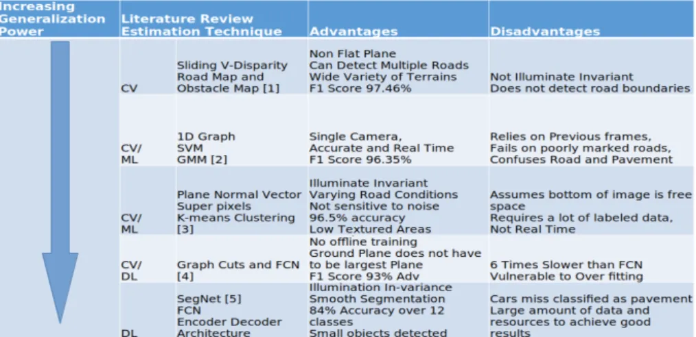
Figure 2.5: Overview of literature review

An overview of the literature review has shown that deep learning techniques have the best generalization power. The are able to accurately segment numerous different classes, and even individual lanes. As semantic segmentation seeks to

(28)

2 Literature Review

achieved full image understanding, it is important to use numerous classes. Furthermore may different objects will present themselves in autonomous driving scenes. Deep Learning is capable of learning complex driving decisions. It is important to identify objects and also where. Deep learning has the ability to deliver on all of these requirements. From the table we can see that deep learning achieves a very good result in identifying numerous different obstacle classes. A thorough free drive-able space application needs to accurately identify and classify all available objects. This would be the basis of the proposed system however classic computer vision techniques must not be neglected as they are capable of a very high pixel wise precision.

(29)

3 Technological Background

As noted in the literature review deep learning offers the best advantages for full frame semantic segmentation. Deep learning is a highly complex and rapidly advancing subject. Before implementing a Deep learning system it is first necessary to gain a thorough understanding of the principals underpinning deep learning and artificial intelligence. This chapter, will start with the basics of deep learning which is Artificial Neural Networks. Next Convolutional Neural Networks (CNNs) will be considered. CNNs have been highly successful in image

recognition-tasks, however CNNs disregard spatial information, which is necessary for accurate segmentation. Fully Convolutional Networks (FCNs) will then be presented as a solution to this issue. FCNs are remodeled CNNs for the task of semantic segmentation. Subsequently transfer learning will be considered. Transfer learning significantly boosts Deep Leaning approaches. Finally Monocular Depth will be briefly reviewed. Monocular depth allows depth estimation from a single image, and like other Computer Vision problems its performance has been greatly improved from deep learning techniques.

3.1 Multi Layer Perceptrons Networks

A biological neuron consists of 4 major parts namely Dendrites, Nucleus, Axon and Axon terminals. The Dendrites accept inputs, the Nucleus processes inputs the Axon carries inputs along the cell body while the Axon terminals connect to other neurons as per Fig[3.1].

An artificial neural network is a mathematical model of a biological neuron. The Artificial neuron consists of the following, Inputs, Weights, Bias and Transfer functions. Inputs are multiplied by a weight and summed up. The Bias is added then the result is passed through an activation function. The activation function is the threshold that the neuron will activate at as per Fig[3.2].

(30)

3 Technological Background

Figure 3.1: Biological Neuron

Figure 3.2: Mathematical Model

Neurons can be combined together to form a network, a row of neurons is called a layer. A network has one input layer one or more hidden layers and one output layer. An output layer is also referred to a logits layer. Neurons can be placed together to form a multi-layer perceptron, where each neuron provides inputs for the neuron in the next layer. In a simple example the network consists of an input layer, a hidden layer and an output layer. The input or visible layer takes inputs from the data-set, for example images. This layer will typically find low level features in the data-set such as edges. The next layer is the hidden layer. This layer is so called as it is hidden from the datasets. Deep Networks have more than one hidden layer. Typically this layer would take edges as input and begin to put the edges together to find patters. The final layer is called the output layer. This layer is responsible for outputting a value. The choice of activation function used in this layer depends on the problem at hand. A binary classification problem could only have one neuron that outputs a value between 0 and 1. A multi class classification problem may have a neuron for each class, in this case a softmax

(31)

activation function would be used. Multi Layer Preceptron Networks are also known as feed forward networks, one forward pass of the data set through the network is called an epoch.

Figure 3.3: Multi Layer Preceptron Networks[15]

Training the Network

In order to train the network labeled data is necessary. The difference between the actual result of the output layer and the expected result is subtracted and this is the error. A loss function is defined to measure the error. In order to minimize the error Gradient decent is used, As per figure [3.4]

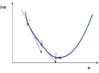
Gradient Decent

Gradient decent is used to minimize the error. This is done by using a function to plot the error and respective weight of a neuron on a graph. The Slope is defined as the difference between two points. If the minimum of the function is to the left of the current position then the slope will be positive and conversely if the

minimum lies to the left then slope will be negative. The weights are moved to check the reduction in the error, then the path of the steepest descent is taken. the algorithm continues to iterate until it converges at a minimum. The minimum is always a local minimum however it is not always a global minimum. In summary Gradient decent is used to minimize errors by adjusting weights.

(32)

3 Technological Background Learning rate

The parameter is called the learning rate or step size. The learning rate is the step that the controls the step that gradient decent function will take to converge to the minimum of the function. If the learning rate is too big the algorithm will not converge at the local minimum, rather it will drift around the local minimum. If it is too small the algorithm will need a lot of steps to converge. Typically the

learning rate is set to a small value such as 0.1 or even 0.01. Additionally, further parameters can be set to complement the learning rate these are momentum and learning rate decay. Momentum stores parameters from previous weight and error updates. The purpose of this is that, it protects the network from small local minima, and continues to reduce the error in the direction of the steepest gradient. Learning rate decay, reduces the learning rate over epochs, it allows large changes to be made at the start and smaller changes later in order to fine tune the network.

Back propagation

The error is used to determine how much the weights have to be changed. This error is back propagated through the network. The chain rule is used to see how changes in one neuron effect changes in other neurons. Nodes that have the

highest impact will be adjusted. Back propagation is used to back propagate error through the network. So first, for each output neuron it is quite obvious, error depends on the difference between expected result and actual result.

For the hidden neuron the error depends on all of the connections between the hidden neurons and output neurons which they connected to. So if in some

connection there is a big weight the hidden neuron error will depend more on that connection if weight is small, less. The hidden neuron error will be the sum of all of the output neurons errors which are connected to this hidden neuron. If one computes the errors they can be used to update the weights. The Gradient decent error value is minimized. Error and weights are adjusted by the amount or error. Another parameter can be set to control the weight updates these are known as batch and online. In online learning weights are updated at every epoch of the data set. This can lead to a disordered and unstable changes to weights, however is has the advantage that it is fast and does not consume much memory. Another version of learning is Batch learning, this is where all errors are computed over the whole dataset and processed at the end, and this type of learning is more

(33)

structured however is it computationally intensive. A trade off between the two methods is mini batch learning, this is also known as Stochastic gradient decent. This is where the data set is broken down into smaller data sets and weights are updated at the end of every batch.

Activation Functions

An activation function is an essential part of each neuron, they are necessary as a neuron’s output must reflect the strength of the weighted sum of its inputs. Older transfer functions such as TanH, Softmax or the sigmoid function take a number as input and return an output between the ranges 0 to 1 in the case of a sigmoid function, and -1 to 1 in the case of a Hyperbolic Tangent function, therefore it’s derivative is stronger than the sigmoid function. The Sigmoid function is

computationally expensive as it must calculate the exponent. Both of these

activate functions suffer from a vanishing gradient problem, this is where gradients get weaker in deep layers of the network, this increases the time to train a model and also reduces its accuracy. A Softmax function is used in the output layer, it takes output values from all neurons in the last layer and returns a probability value ranging from 0 to 1. A ReLU activation function stands for a Rectified Linear Function. A ReLU changes all negative values to 0 and returns all positive values unchanged. An advantage is that a ReLU function is computationally inexpensive, and allows SGD to converge faster. It also prevents gradients from getting smaller in deeper layers. One disadvantage however is that node can quickly become deactivated. A ReLU function is only used in the hidden layers of the network. Traditional activation functions such as Sigmoid, TanH or Softmax are used on the output layer. A Leaky ReLU attempts to prevent nodes from becoming inactive. The principal is the same as ReLU however when the input is negative it returns a small negative value.

(34)

Figure 3.4: Gradient Descent

The Error is minimized my making changes in the weights

3.2 Convolutional neural Networks

As Convolutional Neural Networks can be complex I will first give a general overview and then discuss each major part of the network in detail. A

convolutional neural network is a deep neural network with more than one hidden layers. For example if the dataset consisted of images, the first layer takes raw images as input. The first layer starts to detect features for examples edges. The Second layer puts edge patterns together to form noses eyes the next layer puts these features together to form faces. A simple CNN will consist of the following layers, Convolution, Max Pooling and Fully connected. Firstly the convolution layer will be considered.

Convolutional Layer

Convolution involves sliding a filter across an image, as per Fig[3.5] Multiply each image pixel by the corresponding feature pixel. Add up the result of the

multiplications. Divide by the number of pixels in the feature, finally assign results to the feature map.

The first convolutional layers takes raw 2D array of pixels as input, or 3D array in the case of a RGB image. This layer will accept input as w*h*d where w is the width, h is the height and d is the depth of the image. The convolutional layer will break the image down into smaller features. It will then convolve the image with

(35)

Figure 3.5: Convolution Operation

these features. Line up the feature or small part of the feature and the image patch. Convolving the image has the following steps. Multiply each image pixel by the corresponding feature pixel, this will be done for all RGB channels of the image. Next add up the results of the previous multiplication Finally Divide by the total number of pixels in the feature. As per figure [3.6]

Figure 3.6: Feature Maps

The feature will be multiplied with all values in the original image. This will result in a feature map. The feature map is a way of representing the probabilities that this feature exists at this part of the image. This is necessary as features may be rotated, blurred or scaled. The number of features is equal to the number of feature maps. If the feature does not match well at a certain point is will give a 0.55 or less. This is what the feature map represents, the probability that the feature is present at this location. Stride and padding are hyper parameters which need to be defined. Stride refers to the number of pixels that the filter moves over before performing a matrix multiplication. Padding refers to the number of pixels at the boarder of the images that are ignored.

(36)

The Height and width of outputs can be calculated as follows

Figure 3.7: Output Height Dimensions

Figure 3.8: Output Width Dimensions

Where

Ho and Hi are the images height input.

Wo and Wi are the images width input.

F is the size of the filter

P is the padding parameter

S is the Stride parameter

Max Pooling Layer

The number of parameters can quickly grow due to convolution operations, as every feature results in a feature map. it is necessary to reduce these parameters however whilst still keeping the most important parameters. This is achieved though max pooling. Max pooling is basically shrinking the image but keeping all of the most important values. The following steps are involved. First a window size needs to be defined. For example 2*2. Slide the window across the image and take the maximum value of every pixel of a 2*2 square or the average value can be taken. The stride is defined as the number of pixels that the window is moved at a time, this parameter is different to the convolution step as the stride parameter will decide the output of the sub sampled feature map. The result of this step is a visual similar image with much less pixels. The input is a feature map and the output is a smaller feature map, with all of the most important or most prominent features.

(37)

3 Technological Background Normalization

The outputs of feature maps are fed into ReLU layers or similar activation functions. Using an Activation function such as a ReLu function, in which any non-negative values would be set to 0. This operation is important as image values do not have negative values. Normalization layers are quite simple and have little complexity. Other activation functions such as sigmoid can be used however due to the high computational expense of CNNs ReLu are preferred.

Fully Connected Layer

This layers involves transforming a 2D Array of pixels into a 1D array. The size of this 1D array will be the number of pixels in the last max pooling layer. This list of feature values will be used as probabilities for the final output prediction. It is also possible to have multiple fully connected layers where each predictions will feed the next layer of predictions. A Softmax function is used to return the probability that an object is present in the image. As per MLPs Gradient Decent and Back propagation are used to train the network.

(38)

3.3 Advanced Convolutional Neural Networks

CNNS have developed a lot of interest in recent years, and have attracted a lot of intensive research from academia and IT giants. Developers have raced to increase accuracy, whilst also achieving lower computational demands. One of the key methods to achieve this was to develop different convolutional operations. Convolutional operations are the main reason for increasing the computational complexity of a model, this had subsequently lead to so called bottlenecks in networks. Networks such as Xception and Inception have redesigned convolutional operations into a module and have created the so called network in network structure [12]. Furthermore they have broke away from a traditional sequential form of networks. Much of the efforts in the research problem aim to achieve greater levers of accuracy whilst reducing the number of computations. The Inception network introduced modules as the building block of the network.

Inception V1

Google’s Inception V1 network [23], had a three fold purpose. Like all other advanced Deep Networks they set out to achieve a higher accuracy at the

ImageNet Large Scale Visual Recognition Challenge ILSVRC a coveted prize for object detection. The network achieved a higher accuracy result than the previous winning network with 12 times fewer parameters[23]. However their architecture set out to reduce the computational resource requirements of the network and also achieve scale invariant future extraction. One issue arising the feature extraction is that the same feature can be present a multiple different scales.

A simple form of the original inception module is as per Fig [3.9], it combines convolutions at multiple different scales, for example 1*1, 3*3 and 5*5 convolution operations. This is combined with a max pooling operation in order to reduce spatial density, and finally these convolution operations are combined. To reduce bottlenecks a key tool used was a 1*1 convolution in order to combine channels to the reduce the spatial dimension whilst still keeping the width and height

dimensions. Again this convolution type provides a dual purpose as it also includes a ReLU function A further issue is that 5*5 convolution operations were

computationally expensive. In order to reduce the computational expense 1*1 convolutions were used beforehand.

(39)

3 Technological Background Vanishing Gradient Issue

To Overcome the issue the developers of Deeplab used Softmax classifiers at intermediate stages to overcome this problem.

Evaluation criteria for CNNs is different to semantic segmentation. The standard metric in Segmentation is mIOU whereas in CNNs Top class error is used. This relates to the classification error over the classes predicted. The top score is calculated as the number of times a predicted label matches the target label, divided by the number of instances in the class. This network achieved a new state of the art in detection at the ILSVRC14 with a Top 5 error 10.07 percent. Meaning that the error over the top 5 most accurate class predictions was 10.07 percent.

After Inception V1 the Inception architecture developed in different ways, both attained to the same goal of lowering computational costs whilst also increasing accuracy. I will briefly discuss Inception V2 and V3 along with the Xception architecture. For the most part these architectures aimed at factoring and combining convolution operations. It is important to remember that while the network backbone has not changed, the inception modules have been subject to multiple revisions over new network versions.

Inception v2 and 3

Inception V2 and V3[24] aimed to further the work of V1 in increasing model size and accuracy, while at the same time keeping computational demands low.

Inception had 12 times less parameters than Alex Net , while VGG had 3 times more parameters than AlexNet. [24] Set out to define software engineering principals for the design of CNNs. Firstly the Receptive view should decrease gradually over the network. Higher depth channel dimensions should be processed within an inception block, these high depth channels should be reduced before being convolved by a 3*3 or 5*5 filter. The width and depth of the network should be balanced. Neighboring activation’s in convolution operations should be highly interleave and therefore operations can be reduced before aggregation without loss of information[24]. This network will be considered briefly as it underpins an important theory that is used in State of the Art FCNs. As noted before in inception V1 5*5 convolutions were prohibitively expensive, the authors sought to modify the inception module to reduce develop an equivalent module with the

(40)

same computational costs. The paper explores convolution factorization. In which a 5*5 convolution was replaced with a 3*3 convolution then a 3*1 and a 1*3 convolution, as per Fig[3.9] and [3.10]

Figure 3.9: Original Inception Module

Figure 3.10: Inception Module with Factorized Convolutions

The results of the network were as follows. Top 1 error 21.2 percent and Top 5 error 5.6 percent setting a new state of the art on the ILSRV 2012 data-set.

The Xception network aimed to improve over the inception module, which is a model that achieved a lot of success and inspired many other networks. Xception

(41)

itself has been recreated in many different variants. I will only consider the ones that are relevant to deepab.

Xception

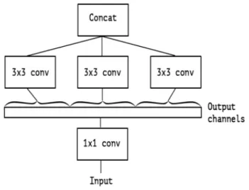
Xception:[7]followed the same software design principals as inception V1 and 2, it sought to increase accuracy while lowering computational requirements. Chollet, invented an Application Programming Interface for rapid experimentation with different inception modules. In doing so he developed the Xception module as per Fig [3.11]

This is a strictly equivalent module to the original inception module. He further improved on this design, to formulate the Xception module which is an extreme version on the inception module as per Fig[3.12]. Furthermore he simplified the Xception architecture.

Figure 3.11: Equivalent module to Original Inception

The network achieved marginal gains on the ImageNet classification task and large gains on the JFT data which is google’s internal dataset.

(42)

Figure 3.12: Extreme Version of Original Inception

3.4 Fully Convolutional Neural Networks

In this subsection I will outline the rational for developing a FCN. Furthermore I will outline the methods of up-sampling and convolutions, which like CNNs are a key aspect of FCNs. I will then look at modifications made to CNNs in order to develop a FCN. I will then give an overview of the functionality of FCNs and the respective architecture. Finally I will discuss the merits of this approach.

Long et al [13] introduced a new type of network specifically developed for Semantic Segmentation. It is based on a remodeled CNN, where all fully

connected layers are turned into de-convolutional layers. It sets a new state of the art for semantic segmentation. It also offers numerous advantages such as being able to accept input of any size, improving computation time and increased accuracy. It redefined segmentation networks and became the architecture of choice for future developments.

Segmentation has an inherent issue, between detection localization and

classification. In a convolutional neural network an image is convolved and down sampled multiple times, this results in CNNs achieving excellent classification however they discard spatial coordinates. The fully connected layers in CNNs are similar to full image convolution, they take image input at any size and return a prediction. Fully connected layers are suitable for Semantic Segmentation, as there is no loss of spatial information, furthermore as ground truth is compared to

(43)

prediction training is easier. The authors in [13] investigated fully connected layers, and in doing so created a FCN, a network that is capable of processing a full image of arbitrary size at a time and returning prediction.

Method of up-sampling

Up-sampling is a key issue in FCNs to retrieve spatial information. In order to retrieve spatial information the authors needed to devise a method of up-sampling the image.

Shift and Stitch method

Involves taking a down sampled image with a known down sampling factor, using the sampling factor to up sample the image. As per Fig[3.13], the filter shifts a number of spaces relating to the up-sampling factor and stitches the pixels to the original image.

Figure 3.13: Shift and Stitch

Another more efficient implementation is the a trois algorithm or hole algorithm, it produces the same results with less computational resources. The filter is spread across a wider space by inserting zeros between the filter. As per Fig [2.10] the convolved pixels are the same as the red pixels in Fig [2.9].

Linear interpolation can also be used to up-sample an image, the method involves taking the nearest neighbors from a pixel value and using these values to up-sample the image. The final method that the authors devised was de-convolution, which is essentially a backwards convolution operation, it is simple to implement and achieved the best results. Therefore this method was implemented in the network.

(44)

Figure 3.14: Altrois Convolution

Loss and training batch size

The authors added further innovations in loss and batch size. Batch size is

breaking a data set down into smaller data sets. The receptive filed, is the number of connections in an image between higher layers and lower layers in the

network[13]. Convolution computes loss on all parts of the image. If all receptive fields are covered in filter wise convolution is the same as whole image convolution. Whole image is better than filter wise training with batches, as it produces the same result as filter wise convolution but faster. As there is substantial overlap in receptive fields, this corresponds to an increased computation time

performance[13].

In order to remodel a CNN to a FCN it is necessary to first remove the final classification layer, this may be a softmax probability or a linear function. Next all fully connected layers are turned into de-convolutional layers. A 1*1 convolution operation is added at every grid as this acts as a classification predictor. As there are 21 classes in Pascal VOC segmentation data-set 21 1*1 convolution operation were added. VGG16 was seen as the best network backbone as it delivered the better result, over Inception and Alex Net.

(45)

Figure 3.15: Fully Convolutional Network Architecture

As an efficient method of up sampling was achieved by de-convolutional layers, the authors needed a method of combining lower layers with higher layers. A skip architecture was designed for this purpose, it is capable of combining the advantages inherent in low highly probable predictions and also, higher finer layers. It can combine deep and shallow features. It also provides a trade off between predictions and fine image boundaries.

Different variants of the FCN exist. They are namely FCN 32, 16 and 8. In a FCN 32 prediction one will be up-sampled and fused with de-convolution three and this will be used as the final output. In a FCN 16 Prediction two will be de-convoluted and fused with Prediction two, this will then be used as the final output. Similarly FCN 8 operates by the same principal as per fig [3.15].

Class balancing

This is a techniques used in Segmentation, where a large part of the labels consists of one label, for example 75 percent of all pixels in a data-set are background. In this case background class can have its weight automatically reduced by 75 percent. This was used in this experiment however it made no difference.

Final Results

The Network achieved a result of 62.7 percent mIOU on the Pascal 2011 and 62.2 percent mIOU on the Pascal VOC 2012 respectively. The results set a new state of

(46)

the art in semantic segmentation, however the most important aspect is that a new type of network with many new innovative features was developed specifically suited to semantic segmentation was developed.

3.5 Advanced Fully Convolutional Networks

This section will give a through examination of a state of the Art FCN namely Deeplab. The development of Deeplab from V1 to V3 will be considered.

Deeplab V1

Deeplab V1 is the state of the Art in Semantic Segmentation [5]. DCNNs suffer from bad localization resulting from repeated convolution and max pooling layers. Their solution was to combine the output of of the DCNN with a Conditional Random Field. Deeplab also implemented the Hole Algorithm which is a special type of convolution filter that can increase the filed of view. An illustration of the hole algorithm is given in fig [3.14]. [13] Did not benefit from this type of

convolution, however Deeplab uses Xception as a network backbone, which can combine features at different scales.

Deep learning offers superior performance in contrast to classical Computer Vision methods such as Histogram of Orientated Gradients and Spare Invariant Feature Transform. Although Deep Learning is invariant to local feature transforms, issues still persist such as the loss of spatial context, and reduced image resolution. Deeplab’s solution to this is the altrois (with holes) Convolutions. Altrois Convolutions allow the Field of View to grow exponentially whilst the computations remain the same.

Spatial accuracy vs classification accuracy is normally a trade off that has to be mitigated when fine tuning a deep learning system. Deeplab’s solution was to use Conditional Random Fields. CRFs have the ability to combine class score

probabilities with low level edge boundary information to provide a sharper segmentation result. Combining these two technologies Altrois Convolutions and CRF resulted in an accuracy increase of 7.28 percent compared to the state of the art and also a processing rate of 8 frames per second.

(47)

3 Technological Background Retrieving Spatial Information

As outlined DCNNs suffer from a loss of spatial information. Deeper CNNs with more convolution and max pooling layers provide better object recognition and however at the cost of reduced pixel accuracy. Research in the issue generally followed two different paths, either a super pixel approach [16] or up sampling and concatenation at different layers[13] or up sample and concatenate predictions at various intermediate steps in order to prevent a loss of spatial information and achieve sharper image boundaries. Deeplab uses a novel approach, DCNNs are used for object recognition, and their output is fed into a Conditional Random field to sharpen the objects boundaries.

Conditional Random Fields

A CRF is a probabilistic graph based method for semantic segmentation. CRF refine the course output of classifiers. A fully connected CRF means that every node is connected in the center, of the graph. Segmentation between nodes is done by means of cost functions. Cost functions are of two types a pairwise and unary term. A pairwise term measures the cost if two neighboring pixels or two pixels with the same color take different labels. A unary term measures the cost if labels disagree with the DCNN classification.

Implementation

VGG 16 network pre-trained on the Image-net data set was used. Using a

pre-trained network is better than random initialization of weights as training the network takes less time, in this case the network took 10 hours to train. The network was modified to convert all fully connected layers into convolutional layers, and convolve the the image at its original size. Next sub sampling is skipped at the last two layers, and altrois convolution is used by adding zeros to the filter. Lastly the 1,000 way classifier is replaced with a 21 way classifier. The image is up-sampled by means of a simple Bi-linear up sampling. Bi-linear

upsampeling applies a filter to the image in order to reconstruct neighboring pixel values that have been lost in down-sampling.

The network achieved a m IOU of 71.6 percent over 21 classes. The Data-set contained 1,464 training examples 1,449 validation examples and 1,456 Testing

(48)

examples. Data augmentation was achieved by adding extra annotated images which resulted in a labeled data set of 10,582. Stochastic gradient decent was used, with a cross entropy loss function. A mini batch size of 20 was used. The initial learning rate was set to 0.001 and was multiplied every 2,000 iterations by 0.1. Finally a momentum of 0.9 was set and a weight decay of 0.0005

Deeplab V2

Deeplab V2 retained Altrous convolution but further improved on the idea by introducing, Altrous Spatial Pyramid Pooling or ASPP. ASPP allows features to be sampled at multiple different fields of view. This technique was combined with a DCNN, and encoder decoder Fully Convolutional Network and a probabilistic graphical method namely CRF. The use of these technologies resulted in an improvement in localization and accuracy. Deeplab V2 achieved a m IOU of 77.69 percent on the Pascal data set.

Atrous Spatial Pyramid Pooling

ASPP involves sampling the image at multiple filters at different fields of view to capture objects at multiple scales in parallel, this was applied to the last max pooling layer. CRF were used in post processing to further refine course output, this technique was carried over from Deeplab v1.

The convolution operation is as follows y [i] = Sum x [i + r.k] w[k]

y[i] is the output x is the input signal

r is the altrois convolution rate, for example in figure 1 the rate is 2 w[k] is the filter of length k

An adjustable learning rate was adding and it is given by the equation (1 iteration / max iteration) exp 2

Two different Altros rates were used namely a small rate 2,4,8,12 and a large rate 6,12,18,24.