Geometric Supervision and Deep Structured Models for Image Segmentation

Thesis for the Degree of Doctor of Philosophy

Geometric Supervision and

Deep Structured Models for

Image Segmentation

Måns Larsson

Department of Electrical Engineering Chalmers University of Technology

Geometric Supervision and Deep Structured Models for Image Segmentation Måns Larsson

ISBN 978-91-7905-294-2 c

_{Måns Larsson}, 2020.

Doktorsavhandlingar vid Chalmers tekniska högskola Ny serie nr 4761

ISSN 0346-718X

Computer Vision and Medical Image Analysis group Department of Electrical Engineering

Chalmers University of Technology SE–412 96 Göteborg, Sweden

Cover:

3D model colored according to (from left): image values, semantic classes and semantic clusters. Related to work done in Paper I and II.

Typeset by the author using LA_TEX. Chalmers Digitaltryck

Geometric Supervision and Deep Structured Models for Image Segmentation Måns Larsson

Department of Electrical Engineering Chalmers University of Technology

Abstract

The task of semantic segmentation aims at understanding an image at a pixel level. Due to its applicability in many areas, such as autonomous vehicles, robotics and medical surgery assistance, semantic segmentation has become an essential task in image analysis. During the last few years a lot of progress have been made for image segmentation algorithms, mainly due to the introduction of deep learning methods, in particular the use of Convolutional Neural Networks (CNNs). CNNs are powerful for modeling complex connections between input and output data but have two drawbacks when it comes to semantic segmentation. Firstly, CNNs lack the ability to directly model dependent output structures, for instance, explicitly enforcing properties such as label smoothness and coherence. This drawback mo-tivates the use of Conditional Random Fields (CRFs), applied as a post-processing step in semantic segmentation. Secondly, training CNNs requires large amounts of annotated data. For segmentation this amounts to dense, pixel-level, annotations that are very time-consuming to acquire.

This thesis summarizes the content of five papers addressing the two afore-mentioned drawbacks of CNNs. The first two papers present methods on how geometric 3D models can be used to improve segmentation models. The 3D mod-els can be created with little human labour and can be used as a supervisory signal to improve the robustness of semantic segmentation and long-term visual localization methods.

The last three papers focuses on models combining CNNs and CRFs for se-mantic segmentation. The models consist of a CNN capable of learning complex image features coupled with a CRF capable of learning dependencies between out-put variables. Emphasis has been on creating models that are possible to train end-to-end, giving the CNN and the CRF a chance to learn how to interact and exploit complementary information to achieve better performance.

Keywords: Semantic segmentation, supervised learning, convolutional neu-ral networks, conditional random fields, deep structured models, self-supervised learning, semi-supervised learning.

Acknowledgements

I would like to start off by thanking my supervisor Fredrik Kahl for introducing me to the field of Computer Vision as well as guiding me through my PhD while constantly having to convince me that what I’m doing is actually worth publish-ing. Your input, encouragement and ideas have been invaluable during this time. Another big thanks to Torsten Sattler, who has been my co-supervisor during the last two years of my PhD. Your never-ending ideas for experiments and inhuman pre-deadline work capacity have been crucial during this time.

I am also grateful for my current and former colleagues in the Computer Vision Group and the department of Electrical Engineering at Chalmers. Thank you Carl Toft, Erik Stenborg, Lars Hammarstrand, Olof Enqvist, Carl Olsson, Christopher Zach, Lucas Brynte, José Pedro Lopes Iglesias, Huu Le, Rasmus Kjær Høier, Georg Bökman, Eskil Jörgensen, Kunal Chelani, Mikaela Åhlén, Yuhang Zhang and Jesús Briales García for you good company, great coffee break discussions and the occasional after work. A special thanks to Jennifer Alvén for starting her PhD a few months before me and hence constantly having to guide me through mine, your help has been much appreciated. In addition I would like to extend my thanks to my collaborators at the Torr Vision Group in Oxford, especially Anurag Arnab and Shuai Zheng who have been involved in the development of the second part of this thesis and introduced me to the wonderful yet frightening world of large-scale deep learning experiments.

Lastly, I would like to thank my friends and family. My family, for continuing to support me in what I’m doing, even though they stopped understanding what it is a long time ago. My friends, for brightening my spare time and constantly reminding me that there are more important and enjoyable things than work. My wonderful girlfriend, Maria, for all her support and constant encouragement in everything I do. Thank you all!

Included Publications

Paper I M. Larsson, E. Stenborg, L. Hammarstrand, M. Pollefeys, T. Sat-tler, F. Kahl ”A Cross-Season Correspondence Dataset for Robust Se-mantic Segmentation”. Conference on Computer Vision and Pattern Recognition (CVPR). 2019.

Paper II M. Larsson, E. Stenborg, C. Toft, L. Hammarstrand, T. Sattler, F. Kahl ”Fine-Grained Segmentation Networks: Self-Supervised Seg-mentation for Improved Long-Term Visual Localization”. Interna-tional Conference on Computer Vision (ICCV). 2019.

Paper III M. Larsson, A. Arnab, F. Kahl, S. Zheng, and P. Torr. ”Revisiting Deep Structured Models in Semantic Segmentation with Gradient-Based Inference”. SIAM Journal on Imaging Sciences (SIIMS).2018. Extended version of paper (a)1_.

Paper IV M. Larsson, J. Alvén and F. Kahl. ”Max-Margin Learning of Deep Structured Models for Semantic Segmentation”. Scandinavian Con-ference on Image Analysis (SCIA). 2017.

Paper V M. Larsson, Y. Zhang and F. Kahl ”Robust Abdominal Organ Seg-mentation Using Regional Convolutional Neural Networks”. Applied Soft Computing. 2018. Extended version of paper (b)1.

Included Publications

Subsidiary publications

(a) M. Larsson, A. Arnab, F. Kahl, S, Zheng, and P. Torr. ”A Projected Gradient Descent Method for CRF Inference allowing End To End Training of Arbi-trary Pairwise Potentials”. International Conference on Energy Minimiza-tion Methods in Computer Vision and Pattern RecogniMinimiza-tion (EMMCVPR). 2017.

(b) M. Larsson, Y. Zhang and F. Kahl ”Robust Abdominal Organ Segmentation Using Regional Convolutional Neural Networks”. Scandinavian Conference on Image Analysis (SCIA).2017.

(c) A. Arnab, S. Zheng, S. Jayasumana, B. Romera-Paredes, M. Larsson, A. Kir-illov, B. Savchynskyy, C. Rother, F. Kahl, P. Torr. Conditional Random Fields Meet Deep Neural Networks for Semantic Segmentation: Combining Probabilistic Graphical Models with Deep Learning for Structured Predic-tion". Signal Processing Magazines Special Issue on: Deep Learning for Visual Understanding. 2018.

Contents

I

Introductory Chapters

2.2.1 Multilayer Neural Networks . . . 10

2.2.2 Activation Functions . . . 11

2.2.3 Convolutional Neural Networks . . . 12

2.2.4 Learning . . . 13

2.3 Learning Structure . . . 17

2.3.1 Conditional Random Fields . . . 17

2.4 End-to-End Learning . . . 22

2.4.1 CRF Inference as a Neural Network Layer . . . 22

2.4.2 Back-propagating CRF Learning Objective . . . 23

2.5 Learning Without Full Supervision . . . 24

2.5.1 Unsupervised Learning . . . 24 2.5.2 Semi-supervised Learning . . . 25 2.5.3 Weakly-supervised Learning . . . 27 3 Summary 29 3.1 Paper I . . . 33 3.2 Paper II . . . 34

Contents 3.3 Paper III . . . 35 3.4 Paper IV . . . 36 3.5 Paper V . . . 37 4 Outlook 39 4.1 Future Work . . . 40 4.1.1 Structured Output . . . 40 4.1.2 Weak Supervision . . . 41 4.1.3 Visual Localization . . . 41 Bibliography 43

II

Included Publications

2 Related Work . . . 61

3 Semantic Correspondence Loss . . . 63

4 A Cross-Season Correspondence Dataset . . . 64

4.1 CMU Seasons Correspondence Dataset . . . 65

4.2 Oxford RobotCar Correspondence Dataset . . . 67

5 Implementation Details . . . 68

6 Experimental Evaluation . . . 70

7 Conclusion . . . 75

References . . . 76

Supplementary Material . . . 84

Paper II Fine-Grained Segmentation Networks: Self-Supervised Segmentation for Improved Long-Term Visual Localization 91 1 Introduction . . . 91

2 Related Work . . . 93

3 Fine-Grained Segmentation Networks . . . 95

4 Semantic Visual Localization . . . 99

5 Experiments . . . 100

5.1 Semantic Information in Clusters . . . 102

5.2 Visual Localization . . . 103

6 Conclusion . . . 106

References . . . 107

Contents Paper III Revisiting Deep Structured Models in Semantic

Segmentation with Gradient-Based Inference 125

1 Introduction . . . 125

2 CRF Formulation . . . 128

2.1 Potentials . . . 128

2.2 Multi-label Graph Expansion and Relaxation . . . 130

3 MAP Inference via Gradient Descent Minimization . . . 131

3.1 Gradient Computations . . . 131

3.2 Update Step and Projection to Feasible Set . . . 132

3.3 Comparison to Mean-Field. . . 133

4 Integration in a Deep Neural Network . . . 133

4.1 Initialization. . . 134

4.2 Gradient Computations. . . 134

4.3 Entropic Descent Update . . . 135

5 Recurrent Formulation as Deep Structured Model . . . 136

6 Implementation Details . . . 137 7 Experiments . . . 138 7.1 Weizmann Horse . . . 138 7.2 NYU V2 . . . 140 7.3 PASCAL VOC . . . 140 7.4 Execution Time . . . 142 8 Conclusion . . . 143 References . . . 147 Supplementary Material . . . 152

Paper IV Max-Margin Learning of Deep Structured Models for Semantic Segmentation 157 1 Introduction . . . 157

1.1 Contributions . . . 158

1.2 Related Work . . . 159

2 A Deep Conditional Random Field Model . . . 159

2.1 Inference . . . 160

2.2 Max-Margin Learning . . . 161

2.3 Back-propagation of Error Derivatives . . . 162

2.4 End-to-End Training in Batches . . . 164

3 Experiments and Results . . . 164

3.1 Weizmann Horse Dataset . . . 165

3.2 Cardiac Ultrasound Dataset . . . 166

3.3 Cardiac CTA Dataset . . . 166

Contents

References . . . 169

Supplementary Material . . . 173

Paper V Robust Abdominal Organ Segmentation Using Regional Convolutional Neural Networks 185 1 Introduction . . . 185

2 Proposed Solution . . . 186

2.1 Localization of Region of Interest . . . 187

2.2 Voxel Classification Using a Convolutional Neural Network . 188 2.3 Postprocessing . . . 193 3 Experimental Results . . . 193 3.1 Runtimes . . . 195 4 Discussion . . . 198 5 Conclusion . . . 199 References . . . 199

Part I

Chapter 1

Introduction

Understanding the content of an image is something that humans excel at. If I were to ask you to describe the objects present in an image you would in almost all cases manage that task effortlessly. However, if I ask you to state a set of rules to decide if an image contains a cat or a dog, you might have difficulties. Humans are so good at parsing and understanding visual scenes that we do not reflect on how we do it. Designing methods that do this automatically has however been proven to be a challenging problem and the field of Computer Vision is still very active.

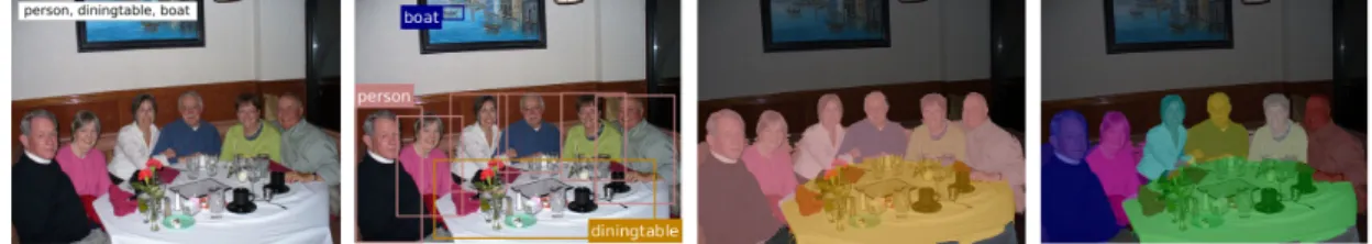
Given an image, information can be extracted on different levels. This is ill-ustrated in Figure 1.1 where a few examples of image analysis tasks of different detail are shown. The focus of this thesis is semantic segmentation, which aims at understanding an image on a pixel level. This means that we want to assign a label to each pixel, describing the object it is depicting. For example, going back to Figure 1.1, we have assigned the label "person" to the pixels colored pink and the label "dining table" to the pixels colored yellow.

Semantic segmentation has numerous of applications. In robotics, agents are usually required to extract useful information and understand their environment to perform tasks such as navigation and manipulation of objects. This is some-thing that can be achieved with a camera and a semantic segmentation algorithm. Also, autonomous vehicles require a precise understanding of their surrounding to be able to make safe decisions in traffic. Semantic segmentation algorithms are also useful for numerous applications in medical research and clinical care, such as computer aided diagnosis and surgery assistance. Since many of the im-ages handled in medical applications are three dimensional manual segmentation is time consuming. Having an automatic method will in these cases save medical personnel a lot of time and be very helpful for time-critical tasks such as surgery planning.

Chapter 1. Introduction

Figure 1.1: Example of scene understanding tasks with increasing detail from left to right. From left: image captioning, object detection, semantic segmentation and instance segmentation. This thesis focuses on semantic segmentation. Image modified from [1].

Traditionally, semantic segmentation algorithms have been approached by ex-tracting some type of hand-crafted image features from the image. These features could be something as simple as a color gradient or a more complex function of the pixel values. A model relating these features to semantic classes is then created, or learnt from annotated examples, i.e. a set of images paired with their "true" semantic segmentations. During recent years most methods have moved from hand-crafted features to using Convolutional Neural Networks (CNNs), capable of learning complex features directly from image data.

The introduction of CNNs for semantic segmentation meant a large improve-ment in performance and we are now able to create models that are fairly good at understanding the content of an image (given that it is similar to the images it has been trained on). A drawback with a CNN is however that they cannot explicitly take the dependencies between output variables, i.e. how the label of one pixel depends on the label of the output pixels, into account. This can however be done using Conditional Random Fields (CRFs), which have been used extensively for semantic segmentation. Because of this, many methods combine a CNN and a CRF creating a Deep Structured Model (DSM) capable of learning complex image features while still taking output dependencies into account.

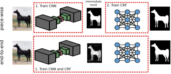
The parameters of these DSMs are usually learnt from data. This learning can be easily achieved by using traditional deep learning methods to train the CNN. Then, using the output of the CNN to form the CRF, learning the weight of the CRF. This approach, commonly referred to as piece-wise training, is suboptimal since the parameters of the CNN is learnt while ignoring output dependencies. A better approach is to train the CNN and CRF jointly, or end-to-end. This gives the CNN and the CRF a chance to learn how to interact to achieve better results. A sketch of piece-wise and end-to-end training of a DSM is shown in Figure 1.2.

DSMs and CNNs usually contains many learnable parameters, or weights, which require a lot of annotated data to train properly. For semantic

segmenta-1.1. Thesis Scope piece-wise end-to -end 1. Train CNN 2. Train CRF 1. Train CNN and CRF intermediate result

Figure 1.2: Comparison of piece-wise and end-to-end training of a deep structured model (DSM). For the piece-wise training (above) the CNN is trained first and as a second step the parameters of the CRF are trained keeping the weights of the CNN fixed. During end-to-end training (below) the weights of the CNN and CRF are jointly trained, giving them a chance to learn how to interact to achieve better results.

tion, annotating data is a tedious task meaning that large datasets are costly and time-consuming to acquire. Methods that alleviate the need for densely annotated data can usually be divided into one of the following categories: unsupervised, weakly-supervised or semi-supervised learning. As their respective names suggest unsupervised learning aims at training models without any manually annotated data, weakly-supervised learning with weaker annotations that are easier to obtain and semi-supervised learning where one part of the dataset is annotated and the other contains no labels.

1.1

Thesis Scope

The topic of this thesis is semantic segmentation in Computer Vision. It contains five papers that can be divided into two main parts. The first one being develop-ment of methods to utilize geometric supervision to improve segdevelop-mentation methods and the second one being development of DSMs for semantic segmentation.

The first part consists of two papers, both of them revolving around the uti-lization of 3D models to improve segmentation models. These works contain tools from unsupervised, weakly-supervised and semi-supervised learning that are used

Chapter 1. Introduction

conjunction with geometric 3D models created from images. The geometric su-pervision is used to improve upon semantic segmentation methods or train CNNs that output fine-grained segmentation containing information useful for visual lo-calization methods.

This second part consists of three papers, all of them presenting solutions to semantic segmentation problems. The applications have varied widely and different types of data have been considered, from 3D CT images to RGB images of horses to indoor scene understanding. The main focus has been on developing robust and accurate models to solve these problems. These models consist of a CNN capable of learning complex image features coupled with a CRF capable of learning dependencies between output variable, in our case pixel or voxel labels. Emphasis have been put on creating this type of models that also are possible to train end-to-end as well as the methods needed to enable this type of training.

1.2

Thesis Outline

The first part of this thesis consists of this introductory chapter, followed by Chap-ter 2 that provides background knowledge to the papers included in the thesis as well as placing them in an academic context. Chapter 3 summarizes the work and contributions of the thesis as well as each paper separately. A brief discussion of future work is given in Chapter 4. Finally, the included papers are appended in Part II.

Chapter 2

Background

The background chapter will start off with a brief introduction to the problem of semantic segmentation. Afterwards some background on Convolutional Neural Networks (CNNs) as well as Conditional Random Fields (CRFs) will be given. Following that, end-to-end training of Deep Structured Models (DSMs), i.e. a combination of a CNN and a CRF, will be discussed. Lastly, a section on train-ing semantic segmentation algorithms without full supervision is included. The sections in this chapter are by no means exhaustive but aim at giving the reader enough background knowledge to understand the papers included as well as place them in an academic context.

2.1

Semantic Segmentation

Semantic segmentation, or scene labeling, is the process of assigning each pixel of an image to the semantic class that it is depicting. The semantic class should depend on the surrounding information, or context, of the pixel. That means that we want to understand what the image is containing on a pixel level. What classes we are interested in dividing the image pixel in depends on the task and what information about our surrounding we are interested in. Given a set of images from a camera mounted on the front of a car we might want to classify each pixel as being one ofe.g. "driveable surface", "sidewalk" or "pedestrian" whereas given a medical CT image of the abdomen we might want to classify pixels into different organs, or perhaps "tumour" and "not tumour". An example of visualizations of semantic segmentations is shown in Figure 2.1.

Chapter 2. Background

Figure 2.1: Two examples of semantic segmentations. To the left is an image from the Mapillary Vistas dataset [2], a street-level image dataset with 66 semantic classes. The semantic class of each pixel is visualized by overlaying the original pixel with the class color. To the right is a slice of a CT image from the MICCAI 2015 challenge “Multi-Atlas Labeling Beyond the Cranial Vault” [3] for organ seg-mentation in the abdomen. Here the voxels of a class are visualized by delineating them with the class color. Note that only one slice of the original 3D CT volume is shown.

2.1.1

Evaluation

Given an image paired with a semantic segmentation it is quite easy for a human to visually evaluate the segmentation as good or bad. It is however important to quantify how good a segmentation is, both to be able to quickly evaluate a method applied to a big set of images and also to be able to compare between different methods. A straightforward metric to use is the pixel accuracy which is defined as the ratio between correctly classified pixels and total number of pixels. However, for some datasets, the per-pixel accuracy can be quite misleading. Given, for example, an image with a lot of pixels labeled as "background". A segmentation method simply assigning the "background" label to all pixels will get a high pixel accuracy even though it obviously performs poorly.

An alternative metric is the commonly used Intersection over Union (IoU) or "Jaccard" index. Given the set of pixels A segmented as a class and the set of pixels B belonging to the same class according to the annotation the IoU is

IoU = |A∩B|

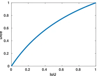
2.1. Semantic Segmentation 0 0.2 0.4 0.6 0.8 1 IoU 0 0.2 0.4 0.6 0.8 1 Dice

Figure 2.2: The Dice coefficient plotted as a function of the intersection over union. The Dice coefficient and intersection over union are two commonly used measure to quantify segmentation results. Note that the Dice coefficient is higher than the intersection over union for any segmentation result.

In terms of true/false positives/negatives we get

IoU= #tp

#tp+ #f n+ #f p, (2.2)

where#tpdenotes number of true positives,#f ndenotes number of false negatives and so on. The IoU is a value between zero and one where a value of one means a perfect overlap of the segmentation and the ground truth while a value of zero means no overlap at all. For multi-label problems the mean IoU (mIoU) over all classes is usually measured as an overall performance indicator of a segmentation method.

For medical image segmentation tasks the Sørensen-Dice coefficient, or sim-ply Dice coefficient, is a common metric. Keeping the notation above, the Dice coefficient is defined as

Dice= 2|A∩B|

|A|+|B|, (2.3)

which in terms of true/false positives/negatives can be written as

Dice= 2#tp

2#tp+ #f n+ #f p. (2.4)

Similarly to the IoU, the Dice score can vary between zero and one. The relation between the Dice score and the IoU is Dice= 2 IoU/(1+IoU)which is visualized in

Chapter 2. Background

Deep Convolutional Neural Network

Input Image

Texton Feature

Extractor Boosting Classifier

Unary Result

Grid CRF

Input Image

Texton Feature

Extractor Boosting Classifier

Unary Result

Dense CRF

Input Image

Convolutional

Feature Extractor Linear Classifier

Unary Result

Dense CRF

Deep Convolutional Neural Network

Input Image

Convolutional

Feature Extractor Linear Classifier

Result CRF Inference Layer

Figure 2.3: Evolution of Semantic Segmentation systems. Initially, most ap-proaches relied on hand-crafted image features and a fairly simple CRF model, this is represented in the first row showing the "Textonboost" work [4]. The second row uses a more sophisticated CRF model, DenseCRF, presented in [5]. Later on, most works have replaced the hand-crafted features with features learned from data with a Convolutional Neural Network. An early example of this is [6]. In [7], it was shown that the CRF inference could incorporated as a part of the CNN. This allowed simultaneous learning of the CNN and CRF weights, further improving results. This image is taken from [1] and result for this figure were obtained using the publicly available code of [6–10].

Figure 2.2. As can be seen from the figure, the Dice coefficient always corresponds to a lower intersection over union.

2.1.2

Development of Approaches

Semantic segmentation methods date back to the 1970s [11,12]. Many of the early approaches tried to divide the image into semantic areas and then relate these areas to each other using a fixed rule-based system. It was in most cases hard to get these kind of rule-based or grammar-based methods to generalize well and performance was quite poor.

From the early 2000s up until now the popularity and performance of semantic segmentation methods have increased tremendously. The early methods utilized

2.1. Semantic Segmentation powerful tools such as image descriptor and machine learning [13]. The majority of these methods are data driven and require manually annotated images to be able to train the models. The models can, once trained, be applied to unseen images and segment them into the semantic classes that were present in the man-ually annotated images. Many state-of-the-art methods [4, 5] used a CRF to be able to model interactions between the input images and output labels but also interactions between output labels. Given a CRF model most early approaches used the following pipeline

1. Extract features from the image, e.g. the RGB color of the pixel and its surrounding pixel or some more advanced features such as Textons [14] or SIFT [4].

2. Use extracted features and the annotated image to train an appearance model, i.e. a local classifier.

3. Use the output of the appearance model to form the unary term, i.e. the part of the CRF that models interactions between input and output.

4. Define, or learn from data, how the CRF should model interactions between output labels. Most commonly the type of interactions were pairwise, i.e. between the classes of two pixels.

5. Perform inference on the CRF model to segment an image.

This is of course a rough pipeline which many methods will not fit into. In addi-tion, a lot of extensions and variants exists for each step of the pipeline. Regarding the first point of extracting features, most work has moved from carefully designed features to learning features from annotated data, usually with a CNN. This will be discussed thoroughly in Chapter 2.2. Also, several works have done data driven approaches to learn the pairwise interactions described by the CRF. In addition, several different types of CRF models have been proposed. A notable example is the DenseCrf presented in [5] where every pair of pixels is connected by a pairwise term in the CRF. Finally, during the last few years methods that learn the param-eters of the CRF as well as the weights of the feature extracting CNN jointly have appeared. Two of them are the papers included in this thesis but more examples exist [7, 15, 16]. Figure 2.3 provides a summary of the development of semantic segmentation systems.

Chapter 2. Background

2.2

Learning Features

As mentioned in Section 2.1.2, most methods for semantic segmentation currently use image features learnt from annotated data. The dominating approach is to apply a CNN to learn these features and inspecting most popular semantic seg-mentation benchmarks, top entries on the leaderboard all use a CNN. In this section an introduction to Artificial Neural Networks (ANNs) and CNNs is given. The idea behind ANNs and CNNs is not new. Already in the 1960s the bio-logically inspired Perceptron was introduced [17] which resembles the commonly used ANNs of today. Also the idea of introducing spatial invariance in ANNs were presented already in 1980, when K. Fukushima et al. introduced the "Neocogni-tron" [18]. During the 1980s and 1990s there was some progression in the field of neural networks but it was not until 2012 that these types of methods got their breakthrough. In 2012 Krizhevsky et al. [19] presented "Alexnet", a CNN for classifying images of the ImageNet [20] dataset that achieved considerably better than the previous state-of-the-art. Since then, approaches using CNNs have be-come dominant in most detection and classification problems [21]. For the task of semantic segmentation a defining paper was J Longs et al. "Fully convolutional networks for semantic segmentation" [10] which introduced a method of trans-forming CNNs previously used for classification to efficiently segment an image. These types of "Fully Convolutional" networks has since then been standard for semantic segmentation.

2.2.1

Multilayer Neural Networks

The most common ANNs have a "feed-forward" neural network architecture. In feed-forward neural networks computations are done layer-wise, and the values of the data at one layer of the network depend only on computations in previous layers. In one layer of the network, the input to the layers is multiplied by a weight vectorWi and a bias vector is added bi according to

gi =Wihi−1+bi, (2.5)

where hi−1 is the output of the previous layer (or the input data if i is the first

layer). The vectors hi are commonly referred to as hidden units (except for the

inputsh0 and the outputhL), or neurons, and their size depends on the size of the

weight matrices Wi. A weight matrix with less rows than columns will decrease

the size of the hidden units vector. After this computation the outputgi is passed

through a non-linear activation function

2.2. Learning Features Computation layers are stacked on top of each other and the output of the last layer L is the output of the neural network y = hL. In modern literature, these

types of neural network layers are often referred to as fully connected layers.

2.2.2

Activation Functions

Activation functions are a crucial part of the neural network. If activation func-tions were to be omitted the computafunc-tions of the entire network would consist of only linear functions and could be replaced with an equivalent single matrix mul-tiplication. In contrast, with non-linear activation functions, it has been shown that a feed-forward neural network is a universal function approximator [22]. This means that, in theory, they can learn any function.

In the early days of neural networks, smooth non-linear activation functions were commonly used. Two examples of these are the sigmoid, defined as

σ(x) = 1

1 +e−x, (2.7)

and the hyperbolicus tangent function σ(x) = tanhx. These functions are quite similar but differs in range, the output of a sigmoid lie within ]0,1[ while the output of tanh(x) lie within ]−1,1[. The rectified linear unit (ReLU) [23], which is defined as σ(x) = max(0, x), is a commonly used activation function. Including ReLU activation functions in a neural network generally makes the training faster as well as allowing training of networks with more layers [21].

The activation function of the final layer is usually chosen differently to the intermediate activation functions. The choice usually depends on what task we are training the network to solve. For example, if we want to use the network to solve a regression problem we might not use any final activation function at all, allowing for unbounded output values of the network. If we instead are interested in image classification we could use a softmax activation function defined as

σ(x)j =

exj

PC

k=1exk

for j = 1, ..., C. (2.8)

The softmax function outputs a set of values all between zero and one and which sum to one. The value of σ(x)j can hence be used as an estimation of the

Chapter 2. Background

2.2.3

Convolutional Neural Networks

Convolutional Neural Networks [24] are designed to process data that has an in-herent grid-like structure, such as 2D RGB images, 3D videos or medical images such as CT scans. Since many of these data types have a lot of input para-meters, an RGB image of standard size can for example be represented with

512×512×3 = 786432values, the weight matrixW of a fully connected layer would

become very large. This would make the computations very demanding while also giving the neural network an extremely large amount of weights, something that might cause overfitting.

CNNs circumvent this problem by using a biologically inspired spatial weight sharing scheme [25]. Instead of learning full weight matrices for each layer a CNN learns a bank of filters for each convolutional layer. The intermediate values between layers are referred to as feature maps and keep their spatial grid-like structure throughout the network. Learning filters, instead of full weight matrices, means that the same weight values will be applied at every spatial position for each layer, greatly reducing the number of weights needed to be learnt. This would be the equivalent of restricting the weight matrix of equation (2.5) to be a Toeplitz matrix. In addition, the convolutional layers are spatially invariant, meaning that input patterns found in different parts of an image will be processed similarly regardless of spatial position.

Another common component of a CNN are pooling layers. A pooling layer applies a rectangular window to each feature map forwarding for example the maximum number present in the window (for max-pooling layers). Pooling layers introduces an invariance to small shifts in input data while also reducing the spatial size of the feature maps, controlling the capacity of the neural network [21]. Adding pooling layers also enlarges the receptive field of higher level features. The receptive field of a feature is the part of the input image that might influence the value of the feature, a larger receptive field enables learning of more complex features. A common approach to building an CNN for image classification is to stack a couple of convolutional and pooling layers, adding activation functions (typically ReLU) after the convolutional layers. This enables the CNN to learn more complex and high-level features for each stacked layer. Ideally the first few layers learn to extract low level image features such as edges, lines and blobs while later layers extracts complex features such as faces, legs or wheels. Finally one or several fully connected layer can be applied to transform the features from spatially structured maps to for example a vector of estimated class probabilities.

2.2. Learning Features Convolutional Layers

As mentioned, the convolutional layers of a CNN each learn a bank of filters. Given an input feature map X of size Win_×Hin_×Fin_{, where W is the width, H the}

height and F the number of feature maps. A trained bank of filters is applied according to

Yj =Bj+

X

i

Wij∗Xi, (2.9)

where Xi denotes the i-th feature map of X and Wij denotes the values of the

learnt filters. The output feature mapY has a size ofWout_×Hout_×Fout_{, padding}

can be used to keep the same width and height as the input feature map. The filter bank has a size ofK1×K2×Fin×Fout, whereK1×K2 is the size of each filter.

For each output, optionally, a bias weight is learnt. Bj denotes this bias resized

to the width and height of the output feature map. The size of the filters differs from application to application but a size of 3×3 is most commonly used [26–28]. A variant of the convolutional layer designed to provide a greater increase of the receptive field (the region of the input that affects a particular unit of the network) between subsequent layers is the à-trous or dilated convolutions [29]. These convolutions uses a set of upsampled filters where only weights at everyl-th index is non-zero. Here, l is usually referred to as the dilation factor, note that dilated convolution with l= 1 is just standard convolution.

Pooling Layers

Pooling layers perform down-sampling of the image features [30]. Several types of pooling layers exist, the most common ones are max pooling and average pooling. These layers applies a fixed size window to the input feature map in strides. It then outputs the max (or average) of the values in this window. Choosing a stride equal to the window size results in non-overlapping regions that forwards information to the next feature map. Choosing a window size of 2×2 and a stride of 2 would result in a down-sampling of the spatial size of the feature map by a factor of 2.

2.2.4

Learning

Once the architecture of our CNN is set we can view it as a function approximator f(x,θ), where x is the input and θ the learnable weights of all layers. This section will give a brief introduction to the most important parts needed for the learning process. Note that this is only applicable for supervised learning, where an annotated dataset is available.

Chapter 2. Background Loss Function

A loss function is a way to quantify how well the CNN is performing, measuring the compatibility of the CNNs output, or prediction, to the ground truth label. The loss is generally defined for one sample of the dataset, and during learning the weights of the CNN,θ are adjusted to minimize the mean of the losses

L(X,Y,θ) = 1

N X

i

l(yi, f(xi,θ)). (2.10)

HereX,Y are the set of input and labels of a given dataset with N samples and

xi, yi denotes the data/label pair of one sample.

A commonly used loss function for classification tasks is the cross-entropy loss. For a CNN with a softmax activation function as a last layer, outputting an esti-mate of the probabilities of the inputxi belonging to each class, the cross-entropy

loss may be defined as

l(yi, f(xi,θ)) =−log(fyi(xi,θ)). (2.11)

Here, fyi(xi,θ) is the estimate of the probability from the CNN that the input

belongs to the ground truth class yi. The name cross-entropy loss comes from

the fact that this loss minimizes the cross entropy between the distribution of the ground truth labels and the label distribution generated by the CNN, given that the samples are independent and identically distibuted random variables.

Loss Minimization

As previously mentioned, the learning is achieved by minimizing a defined loss function over the given dataset. Since there generally is not any closed-form so-lution to the learning problem, θ∗ = arg max(L(X,Y,θ)), local optimization methods are often used. Commonly, a variant of gradient descent is used which updates the parameters of the CNN according to

θi+1 =θi−η∇θL(X,Y,θi), (2.12)

whereηis the step size or learning rate. For large datasets this is however inefficient and a stochastic approximation of the gradient can be used instead. This is called mini-batch gradient descent and is defined as

θi+1=θi−η

X

i∈B

∇θl(yi, f(xi,θi)), (2.13)

where B is the batch which in turn is a subset of the complete dataset. Using a mini-batch of size one is referred to as stochastic gradient descent. There are

2.2. Learning Features several variants of this update rule, designed to reduce noise of the estimated gradient and accelerate convergence. Some examples are gradient descent with momentum [31], with Nesterov momentum [32], AdaGrad [33] and Adam [34]. All of these are first-order methods which means that they only require the calculation of the gradient with regards to the weights.

The gradient of the loss function with respect to all the weights of the network can be efficiently computed using the back-propagation algorithm [31] – a practical application of the chain rule for derivatives. Given the loss derivative ∂L_∂y with respect to the output of a simple layer described by y = f(x, θ), where x is the input, y the output and θ the weights. The loss derivative with respect to the input can calculated by simply applying the chain rule ∂L_∂x = ∂L_∂y∂f_∂x, similarly for the weights we get ∂L_∂θ = ∂L_∂y∂f_∂θ. Using this back-propagation we can start from the final layer of the network and calculate the loss with respect to the input of each layer, propagating the loss gradient all through the network until we have calculated it with respect to every weight of the network.

Since the learning problem is non-convex and almost all methods are based on local optimization it is a possibility for the learning to get stuck in a poor local minimum. In practice, this is generally not a big problem, even for different initial conditions many networks reach a solution of very similar quality [21]. Recent work points towards the existence of a lot of saddle points in the loss surface that the learning algorithm might get stuck in [35, 36]. However, all of them have very similar and low values of the loss function and hence give a good enough solution.

Regularization

Overfitting is a term used for when training a model makes it perform well on the training data but poor on unseen input data. Since a typical CNN contains a very large number of free parameters it is prone to overfitting. A large enough CNN could "memorize" the training data instead of learning good rules that generalize to unseen data. Because of this, several regularization methods meant to prevent the CNN from overfitting have been developed.

Ideally, we would like to just add training data until the CNN is incapable of overfitting. Annotating new data is however a timely process which we generally want to avoid. An alternative to adding new training data is to perform data aug-mentation on the already available data. This means changing the samples of the data slightly in an randomized way during training. Common augmentation oper-ations used for image tasks are, random cropping of the image, random rotation or simply adding noise to the pixel values.

Chapter 2. Background

Another fairly simple regularization technique is weight decay. This means adding an extra term to the loss function that penalize large values of the para-meters of the CNN. For the case of L2 _{weight decay the term λ}1

2

P

iθi2, where

λ is the weight decay strength, is added to the loss function in (2.10). For L1

regularization we instead add the term λP

i|θi|, favoring sparse solutions.

Two additional, very popular, regularization techniques are Dropout [37] and Batch Normalization [38]. These are added as separate layers to the CNN and have different functionalities during learning and during inference. Dropout works by only keeping the values of each neuron non-zero with given probability p, the others are set to zero. During inference, all neuron values are kept but scaled with a factorp. Batch Normalization shifts the values of the features to have a specific mean and variance for each mini-batch during training. In addition to avoiding overfitting to some extent, this also allows the use of a higher learning rate during training [38].

CNNs for Semantic Segmentation

The task of annotating data is considerably harder and more time-consuming for semantic segmentation where each pixel need to be annotated, compared to image classification where only one label per image is needed. This restricts the size of available datasets for semantic segmentation and there are no available datasets of the same size as for example Imagenet [39], which contains millions of annotated images. Due to this, many popular CNNs for semantic segmentation have a classification counterpart that has been trained on the million images of Imagenet. The architecture of the classification CNN is then changed to enable dense output maps, transforming it to a segmentation CNN. The weights of the first few layers are however kept, with the motivation that these layers have learnt to extract meaningful image features during the extensive classification training. This approach have shown to be preferable to training from scratch for many segmentation tasks, even for images fairly different from the Imagenet data [40–42]. Repurposing a classification network for semantic segmentation is not entirely straight-forward. As mentioned in Section 2.2, a defining paper for this was "Fully convolutional networks for semantic segmentation" by J Longet al. [10] where they presented segmentation version of several classification network that were state-of-the-art on Imagenet at that time. The fully connected layers of these networks were transformed to convolutional layers with filter size1×1, which changes the previous classification scores to spatial feature maps. These feature maps, together with feature maps earlier in the CNN were upsampled using deconvolution layers [43] and merged providing dense output predictions for images of arbitrary size. These

2.3. Learning Structure CNNs can then be trained for segmentation end-to-end using a pixel-wise version of the cross-entropy loss presented in Section 2.2.4.

Despite the success of fully convolutional networks of [10] this architecture has several drawbacks. Pooling layers are great for image classification, enabling the CNN to learn complex high-level image features. It is however not ideal since performing pooling operations implies loss of spatial information on where the image features came from in the image. Some works have tried to get rid of the pooling layers entirely [44] and other types of layers have been introduced in an effort to keep spatial information while still achieving large receptive fields. An example of this is the dilated convolutions mentioned in Section 2.2.3.

Many recent works considering CNNs for semantic segmentation try to design networks that are able to learn high-level image features while not losing spatial information. Some examples include encoder-decoder networks such as Segnet [45] and U-Net [46] as well as PSP-Net [47] and DeepLabv3+ [48] that processes features on different resolution in separate paths.

2.3

Learning Structure

As mentioned in Section 2.2.3, CNNs are good at modeling complex relations bet-ween input data and output data. They cannot however explicitly take depend-encies between output variables into account. In addition, they are often trained with a pixel-wise loss function, disregarding the fact that the output data is actu-ally structured.

A way of taking output structure into account while also allowing for explicit modeling of dependencies between output variables is using Probabilistic Graph-ical Models (PGMs). A PGM models a probability distribution over a set of random variables whose structure is defined via a graph. In this thesis we will focus on Conditional Random Fields (CRFs) that are commonly used for semantic segmentation.

2.3.1

Conditional Random Fields

Conditional Random Fields (CRFs) models the conditional probability, P(Y|x)

of a given output set Y = {Y1, ..., YN} and input x. Working with images, x

denotes the image values and we generally associate one input and one output variable with each pixel. For semantic segmentation each output Yi is assigned

a value from a finite set of possible states L = {l1, l2, ..., lL}, where each state

represent a class label. The dependencies between output variables are described by an undirected graph whose vertices are the random variables{Y1, ..., YN}. The

Chapter 2. Background

conditional probability for the CRF can be written as P(Y =y|x) = 1

Z(x)exp(−E(y,x;w)), (2.14)

whereE(y,x;w)denotes the Gibbs energy function with respect to the assignment of labels to the output variables y ∈ LN_{. The parameters, w, of the CRF can}

either be hand-crafted from prior knowledge or learnt from data. Z(x) is the partition function given by

Z(x) = X

y∈LN

exp(−E(y,x;w)). (2.15)

It is hence a normalization constant making the conditional probabilities sum to one. Note that the sum is over all possible combination of label assignments available, it is therefore computationally expensive to evaluate the value of the partition function.

For most image applications the Gibbs energy function decomposes over unary and pairwise terms,i.e. terms depending on only one and two variable respectively. The energy can be written as

E(y,x;w) =X u∈V ψu(yu,x;w) + X (u,v)∈E ψuv(yu, yv,x;w). (2.16)

The terms ψu(yu,x;w) and ψuv(yu, yv,x;w) are commonly referred to as unary

and pairwise potentials respectively. Note that the graph structure defines what terms are present in this energy. For ψuv(yu, yv,x;w) to be non-zero node u and

v must share an edge. Potential Types

The unary potentials, also known as the data cost, of the CRF energy are often obtained from a pixelwise classifier estimating the class probabilities of each pixel. Commonly the term for each pixel is set to

ψu(yu =lp) = −w1log(P(yu =lp|x)), (2.17)

where P(yu = lp|x) is an estimate of the probability of pixel u belonging to class

lp.

For the pairwise potential the connectivity or structure of our graph needs to be defined. This specifies what pairwise terms should be included in the energy, and also which output variables should depend on each other. A simple and commonly

2.3. Learning Structure

y

x

y

x

y

x

y

x

y

x

y

x

y

x

y

x

y

x

y

x

y

x

y

x

y

x

y

x

y

x

y

x

Unary

Pairwise

Figure 2.4: CRF with a simple nearest neighbour connectivity, neighbourhood size four. The variables yu are assigned class labels while the variables xu represents

the pixel values.

used structure is the nearest neighbour connectivity where pixels are connected through an edge to its neighbours only. The size of the neighbourhood might vary but for 2D images a size of four or eight is common. An example of this structure can be seen in Figure 2.4.

The pairwise potentials,ψuv(yu =lp, yv =lq,x;w), defines the cost of assigning

label lp to pixel u and label lq to pixel v. It can hence be used to enforce

consis-tency and structure in the output. As an example, for semantic segmentation, we generally want neighbouring pixels to have the same labels. A type of pairwise term that enforces this is the Potts model given by

ψuv(yu =lp, yv =lq,x;w) =w21lp6=lq, (2.18)

where 1lp6=lq denotes the indicator function equaling one if lp 6= lq and zero

oth-erwise. This pairwise term can be generalized in several ways, for example we might want to weight the cost of assigning different labels to neighbouring pixel differently depending on if they have similar color or not. This can be achieved by adding a weighting term according to

ψuv(yu =lp, yv =lq,x;w) =w31lp6=lqe−(xu−xv)

2

, (2.19)

wherexu and xv are the pixel values of pixeluand v. This type of pairwise terms

Chapter 2. Background

Both of these pairwise terms are constructed using prior knowledge, such that neighbouring pixel often have the same label unless there is a change in contrast. This is of course not true in all cases and several works have instead tried to learn the pairwise term from data [49, 50]. In Paper III we present a CRF model with more general pairwise potentials that can be learnt from data.

Using a neighbourhood only consisting of neighbouring pixels limits the extent on how far across the image information can propagate. A natural way to increase this limit is to increase the size of the neighbourhood, for example connecting all pixels closer than d pixels apart. The extreme of this would be to connect all pairs of pixels which is done for the denseCrf model. The denseCrf model were popularized by [5], that presented a method to perform efficient inference for these types of CRFs. The pairwise terms for dense CRFs also include a weighting on the distance between two pixels, hence the strength of the pairwise term decays exponentially with the distance between the pixels.

It is also possible to include potentials that depend on more than two pixel labels, i.e. higher order potentials. Higher order potentials can for example be used to enforce consistency within superpixels or utilize object detection results for semantic segmentation [51–54].

Inference

The inference problem, giving a semantic segmentation, equates to finding the maximum a posteriori labeling of the model in equation 2.14. Finding the mini-mizer to the Gibbs energy,

y∗ = arg min

y

E(y,x;w), (2.20)

is an equivalent problem. This problem is in general NP-hard [55], typical app-roaches to solving it can hence be divided into two categories, exact algorithms that only apply to special cases of the energy and approximate solutions. We will provide a few examples here but for an extensive overview of approaches we refer to [56, 57].

If we deal with a binary segmentation problem, i.e. only are interested in two classes, and if the energy is submodular the globally optimal solution can be found using the graph cuts method [57]. This approach can be extended to multi-label problems using theα-expansion [58], however we lose the guarantee of finding the global optimum.

Several popular methods are based on a relaxation of the original problem, these are usually the most efficient ones for performing inference in denser CRFs. One example is the mean-field method where the original distribution isP(y|x)is

2.3. Learning Structure approximated with a fully factorized one Q(y). The optimization is then done by minimizing the Kullback–Leibler divergence between the two distributions. Other approaches rely on a continuous relaxation of the Gibbs energy, and then using local search methods to find a local minimum of the energy. This type of methods have been shown to outperform mean-field on several tasks [59] and is the approach used in Paper III.

Parameter Learning

The learning problem consists of estimating the parameters of the CRF,w, based on a training set (y(k)_,x(k)₎N

k=1. The goal with the training is that if inference is

performed for an input image from the data set, we want a solution close to the ground truth labeling. An intuitive approach to the learning problem is based on the maximum likelihood principle,i.e. finding the set of parameters that maximizes the probability of the training set.

A major difficulty when performing maximum likelihood training for CRFs is that it requires computation of the partition function for each training instance and for each iteration of a numerical optimization algorithm. This is of course computationally expensive and makes learning infeasible for CRF models used for semantic segmentation. Most popular learning methods therefore make approx-imations that simplify the computation of the partition function. Mean field is an example of this where the fully factorized distribution simplifies computation of the partition function [5]. Piece-wise training is also an option which only re-quires computation of local normalization factor over fewer variables [60,61]. Other methods instead try to estimate the partition function using sampling [62].

Another approach is to use a learning method that avoids the computation of the partition function, for example learning a model that maximizes the margin between the energy of the ground truth and any other output configuration [63,64]. This can be formulated as

max

w ζ

s.t. E(y,x(k);w)−E(y(k),x(k);w)≥ζ ∀k and y6=y(k).

(2.21)

Since there is an exponential amount of constraints in this optimization problem it is not feasible to solve it as is. A solution to this is to iteratively add the constraints that currently is furthest away from being satisfied [65]. This learning method is utilized in Paper IV.

Chapter 2. Background

2.4

End-to-End Learning

Combining CNNs and CRFs is a powerful approach for dense classification tasks such as semantic segmentation. The CNNs ability to learn complex high-level im-age features paired with the CRFs ability to model output dependencies generally yields impressive results. However, many existing approaches use a two step train-ing process to learn the weights of the CNN and CRF. Firstly, the CNN is trained to perform pixel-wise segmentation on the available data set. Secondly, the CRF is trained keeping the unary potentials fixed (although based on the output of the CNN). This is often referred to as piece-wise training and is non-ideal since the CNN is learnt while ignoring dependencies between output variables.

Instead, a better solution would be to perform end-to-end training. This means jointly training the CNN and the CRF at the same time. In this way the CNN and the CRF get the chance to learn how to interact and exploit complementary information to achieve as good of a result as possible. During recent years several examples of these deep structured model trained end-to-end have been proposed in the literature [7, 50, 66–68]. This section aims at providing a brief introduction to some of these methods, for more details we refer to [1].

2.4.1

CRF Inference as a Neural Network Layer

Given an iterative CRF inference method only consisting of differentiable opera-tions, these operations can be implemented as neural network layers. Each step in the inference routine equaling one forward pass of a network layer. By implement-ing the back-propagation routines for this layer, which amounts to applyimplement-ing the chain rule for derivative, the error derivatives with respect to the parameters of the CRF can be computed during training. In addition, the error derivative with respect to the output of the CNN can be computed and the error can be propa-gated all the way back through the CNN. This enables the parameters of both the CRF and the CNN to be updated simultaneously during learning. This is usually referred to as unrolling inference algorithms and was shown to be possible for the mean-field inference algorithm [7]. In Paper III we show that this is possible for gradient-based CRF inference as well.

2.4. End-to-End Learning

2.4.2

Back-propagating CRF Learning Objective

Many of the approaches for CRF parameter learning presented in Section 2.3.1 can be abstracted to minimizing a global objective L. This global objective depends on the samples of the data set, the parameters of the CRF as well as the output of the CNN, denoted z, used to create the CRF potentials. If we are able to calculate the gradient of this global objective with respect to the CNN output, ∇zL, we can back-propagate this gradient back through the CNN to calculate

∇θL, whereθ are the weights of the CNN. The weights can then be updated using

local search methods. The same thing is possible for the weights of the CRF, if ∇wL is calculated.

This approach of learning is usually formulated as a bi-level optimization prob-lem [69–71] on the following form

min θ N X i=k l(y(k),y∗_k), (2.22) subject to y_k∗ = arg min

y∈C

E(y,z(θ),x(k),w) ∀k. (2.23)

Here,C is the constraint set,Ethe CRF energy and(y(k)_,x(k)₎N

k=1the training set.

Since the optimal solution y∗_k of the inner optimization problem will depend on the output of the network, z, and the weights of the CRF, w, the gradients ∇zL

and ∇wLcan be calculated. In short, for the unconstrained case, this can be done

by applying the implicit function theorem on the first order optimal conditions of the energy function (∇yE =0), and using the fact thaty is a function of z. This

enables the calculation of ∇zyk∗ by solving a linear system consisting of second

order derivatives ofE. Having ∇zy∗kenables back-propagation through the energy

minimization, in this case CRF inference, and hence end-to-end learning.

For more details, as well as the constrained cases, we refer to [70]. In Paper IV we present a method for doing this utilizing the max margin training approach for CRFs introduced in Section 2.3.1. Other examples of methods in this category are [50, 62, 66].

Chapter 2. Background

2.5

Learning Without Full Supervision

The learning approaches presented in previous sections all have one thing in com-mon: they require an annotated dataset. Annotating data for semantic segmen-tation is a tedious task, creating one high-level annotated image can take around 90 minutes [72]. For 3D medical images, annotations are even more time-consuming and costly to acquire since there are a lot more pixels (or voxels) to be annotated and medical expertise is needed. There are several ways of getting around this problem, training neural networks without full supervision. In this section, three prominent categories of these methods will be briefly discussed, namely unsuper-vised learning, semi-superunsuper-vised learning and weakly-superunsuper-vised learning. Note that this is not an exhaustive text on this topic but serves as background to Paper I and II where tools from all three of these categories were utilized.

2.5.1

Unsupervised Learning

Unsupervised learning aims at extracting useful representations and patterns from unlabeled data. In the context of deep learning, this usually equals training the network to output informative features. This is similar to the motivation for pre-training the network on a larger, related dataset as discussed in Section 2.2.4. What counts as informative features depends on what the main goal of the neural network is, hence a common way to evaluate unsupervised learning methods are by applying the pre-trained network on a downstream task. This could, for ex-ample be semantic segmentation where the network that has been pre-trained in an unsupervised fashion is trained for semantic segmentation. The quality of the unsupervised pre-training is then decided by the accuracy and training time of the downstream task.

Autoencoder

An autoencoder is a neural network trained with backpropagation in an unsuper-vised manner [73]. Instead of using annotated labels as training target the autoen-coder is trained to output a copy of the input image, i.e. an autoencoder learns the identity mapping for the training images.

Since this task is trivial, constraints need to be but on the structure of the autoencoder network. A simple way of doing this is to add a bottleneck in the network, i.e. a hidden layer with low dimensionality. In this way the network needs to learn a compact encoding of the input data that contains all information needed for it to be decoded to the original image. The features at the bottleneck of the autoencoder are often referred to as code or latent representation. In the

2.5. Learning Without Full Supervision standard setup, the code has a lower dimensionality than the input data. However, it has been shown that autencoders where the dimensionality of the code is higher than the input also can learn meaningful encodings as well [74]. This by applying regularization to the latent representation.

Self-supervised Learning

In self-supervised learning the annotated labels are replaced by pseudo-labels that can be automatically generated from data. The network is then trained for this pretext task by learning to predict the pseudo-labels. For the network to learn to output useful features, the pretext task need to be meaningful considering the downstream task. Examples of pretext tasks are image colorization [75], image inpainting [76], image jigsaw puzzle solving [77, 78] and rotation prediction [79]. In [80] the pseudo-labels are created by k-means clustering of the output feature vectors. The network is then trained to predict the pseudo-labels. By iterating the k-means clustering and the pseudo-label prediction, the network learns to outputs features useful for several downstream tasks.

2.5.2

Semi-supervised Learning

Semi-supervised learning defines a middle ground between supervised learning and unsupervised learning. In the semi-supervised settings, one part of the available dataset has labels while the rest is unlabeled. Semi-supervised learning seeks to alleviate the need for a large amount of annotated data by allowing a network to leverage the unlabeled part of the dataset. This is generally achieved by adding another loss term during training that can be applied to unlabeled data. These losses can be divided into three main classes [81]: entropy minimization, consis-tency regularization and generic regularization. A short introduction to generic regularization can be found in Section 2.2.4

Entropy Minimization

Entropy minimization encourages the network to increase its confidence on un-labelled data. This is based on the assumption that the decision boundary should not pass by high density regions of the data distribution [82]. In [83], the entropy of the network on output data is minimized explicitly while in [84] this is done implicitly by letting the network create pseudo-labels for the unlabelled data which is then used as targets during training.

Chapter 2. Background Consistency Loss

CNN

CNN

Weight

Sharing

x

ˆ

x

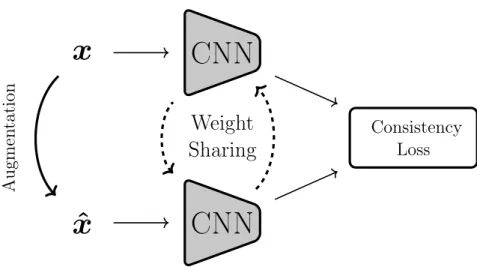
Figure 2.5: A consistency regularization training schematic for semi-supervised learning. The network is trained to produce consistent output for the original input,

x, and an augmented version of the image, xˆ. The assumption made is that the augmentation should not change the labels.

Consistency Regularization

Consistency regularization leverages ideas from data augmentation, generally used as an regularization technique during supervised learning. In data augmentation, a transformation is applied to the input image before being fed to the network. The transformation is often randomized and is designed in a way such that the original labels can be used for the augmented image. A similar approach can be used in the semi-supervised setting for the unlabelled samples. The main idea being that the network should output consistent labels for the original image, x, and an augmented image,xˆ. This is enforced by minimizing a consistency loss over the two outputs, see Fig. 2.5. In this way, the network learns to be invariant to the image changes that can be inferred by the augmentation routines used. In [85] and [86], this consistency is enforced by minimizing the L2 _{distance between the}

outputs of the network forxand xˆ, while in [87] and [88] the network outputs are viewed as probability distributions and the Kullback–Leibler divergence between them is minimized.

Another type of consistency regularization is presented in [89], here a student network is trained to produce consistent output to a "mean teacher" whose weights are an ensemble of a student network’s weights.

2.5. Learning Without Full Supervision

2.5.3

Weakly-supervised Learning

Weakly-supervised learning aims at utilizing weaker, more easily acquired, labels for training. For semantic segmentation weak labels such as image tags [90–95], object bounding boxes [91, 96, 97], points [98] or scribbles [99] have been used to alleviate the need for dense annotations. The general approach is to infer dense labels from the weak labels, the current network output and using additional information or assumptions. An example is [95] where dense labels are inferred by seeded region growing from discriminative regions in the image. The discriminative regions are found by looking for highly activated regions in intermediate feature maps of the network. In [91] both image tags and bounding boxes were utilized in a weakly- and semi-supervised setting. An expectation–maximization method was proposed for training the network using the weak labels.

Chapter 3

Summary

The topics of this thesis revolves around image segmentation, and can be divided into to main parts. The first one being development of methods to utilize 3D geometry to improve segmentation methods and the second one being development of DSMs for semantic segmentation. This chapter includes a summary of these two parts followed by short individual summaries of the papers included in this thesis.

Geometric Supervision for Segmentation

This work started as part of a project addressing the task of semantic localization, i.e. utilizing semantic cues to estimate the pose of a camera given the image taken and an 3D map. One step of the pipeline required accurate semantic segmentations for road-scenarios. What we noticed, when trying some state-of-the-art models trained on the cityscapes dataset [72], was that these performed very poorly on our images. Especially for images taken during different seasons or lighting conditions. In the same project we had created large 3D models of the same localization at different seasons and time of the day. Paper I summarizes our effort to utilize these 3D models to train a CNN that performs well for all image conditions present in the localization dataset, being more robust to seasonal changes and weather conditions. In short, we create a dataset consisting of pairs of images with 2D-2D pixel correspondences. This is done by geometrically matching the 3D models created during different seasons or time of the day. Given the 3D point matches, the pixel positions for the 2D-2D correspondences in each image can be calculated using the camera positions available in the 3D models.

With the insight that two pixels in each 2D-2D correspondence pair should depict the same object, these can be used during training. To this end, we formu-lated a loss function that encourages the output of the CNN to be consistent over

Chapter 3. Summary

every pair of pixel correspondences. This is related to the work on consistency regularization presented in Section 2.5.2, but instead of relying on augmentation methods for creating the input pairs these are created using the 3D models. In this way we can learn the network to be invariant to higher level visual changes, such as summer to winter or day to night.

Creating the dataset of 2D-2D correspondences are not completely automatic and requires some manual labours for the alignment of the different 3D models. Hence, the consistency training across the correspondences falls under weakly-supervised training. This makes the complete training routine used in Paper I both semi- and weakly-supervised. An estimated 30 hours of manual labor was required to create one of the 2D-2D correspondence dataset, which contains 28766 image pairs. This in comparison to the Cityscapes dataset [72], where each image required around 1.5 hours of annotation time.

The segmentation results in Paper I are quite convincing, by adding corre-spondence training we managed to improve upon several strong baselines, even for networks that have been trained on the Mapillary Vistas dataset [2] that is already quite diverse when it comes to variety in lighting conditions and seasons. However, we failed with one of the goals of the work, to show that the improved and more robust segmentation algorithm gave a significant performance boost for semantic visual localization algorithms. Even though there was a small improvement it was less than expected.

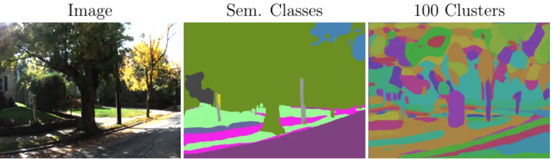
Having segmentations that are consistent across lighting conditions and sea-sonal changes is a crucial part of semantic long-term visual localization. This because the invariance of semantic meaning of the surrounding is one of the as-sumptions made when developing these localization methods. However, in many cases there are only a few classes available that is meaningful for localization. For example, the Cityscapes dataset [72] contains 19 classes, 8 of which cover dynamic objects such as cars or pedestrians that are not useful for localization. The Map-illary Vistas dataset [2] contains 66 classes, with 15 classes for dynamic objects. Hence using semantic labels for visual localization results in a loss of