MPRA
Munich Personal RePEc Archive
Conditional Determinants of Mobile
Phones Penetration and Mobile Banking
in Sub-Saharan Africa
Simplice Asongu
June 2015
Online at
https://mpra.ub.uni-muenchen.de/70235/
1
AFRICAN GOVERNANCE AND DEVELOPMENT
INSTITUTE
A G D I Working Paper
WP/15/043
Conditional Determinants of Mobile Phones Penetration and Mobile Banking in Sub-Saharan Africa
Published: Journal of the Knowledge Economy
Simplice A. Asongu
African Governance and Development Institute, Yaoundé, Cameroon.
2
2015 African Governance and Development Institute WP/15/043
AGDI Working Paper
Research Department
Conditional Determinants of Mobile Phones Penetration and Mobile Banking in Sub-Saharan Africa
Simplice A. Asongu1
October 2015
Abstract
Using twenty-five policy variables, we investigate determinants of mobile phone/banking in 49 Sub-Saharan African countries with data for the year 2011. The determinants are classified into six policy categories, notably: macroeconomic, business/bank, market-related, knowledge economy, external flows and human development. The empirical evidence is based on contemporary and non-contemporary Quantile regressions. The following implications are relevant to the findings. First, mobile phone penetration is positively correlated with: (i) education, domestic savings, regulation quality and patent applications, especially at low initial levels of mobile penetration; (ii) bank density; (iii) urban population density and (iv) internet penetration. Second, the use of the mobile to pay bills is positively linked with: (i) trade and internet penetration, especially in contemporary specifications and (ii) remittances and patent applications, especially at low initial levels of the dependent variable. Third, using the mobile to send/receive money is positively correlated with: internet penetration and human development, especially in the contemporary specifications. Fourth, mobile banking is positively linked with: (i) trade in contemporary specifications; (ii) remittances and patent applications at low initial levels of the dependent variable and (iii) internet penetration and human development, with contemporary threshold evidence. The policy implications are articulated with incremental policy syndromes.
JEL Classification: G20; L96; O11; O33; O55
Keywords: Mobile phones; Mobile banking; Development; Africa
3 1. Introduction
The Sub-Saharan African (SSA) mobile money market which was worth 655.8 million USD in 2014 is currently projected to reach 1.3 billion by 2019 (Caulderwood, 2015). This represents significant opportunities for more financial inclusion, business development and improvement of livelihoods, especially for the previously unbanked segment of the population. Relative to more advanced economies, firms in the sub-region lack proper access to credit facilities. Financing by equity markets is not a feasible alternative because stock markets are still underdeveloped2. The narrative sustains that consistent with the Global Findex Inclusion Database, only 23% of adults living under 2USD/day possess a bank account. Hence, they are more likely to recourse to informal credit alternatives like mobile phone based facilities3.
Mobile phones and mobile banking have been substantially documented to, inter alia: empower women (Maurer, 2008; Ojo et al., 2012), mitigate income-inequality (Asongu 2015ab), promote financial inclusion (Kirui et al. 2013, p. 141; Singh, 2012, p. 466), bridge the rural-urban divide (Qiang et al., 2011, pp. 14-26; Chan & Jia, 2011, pp. 3-5), improve health services for the poor (Kliner et al., 2013), eliminate agricultural wastes by mitigating demand-supply mismatches as well as demand- and supply-side constraints (Muto & Yamano, 2009; Aker & Fafchamps, 2010), enhance business opportunities (Ondiege, 2010, p. 11; Mishra & Bisht, 2013, p. 505) and efficiency in household management (Al Surikhi, 2012; Asongu, 2015c). With growing requests for more research on the development outcomes of mobile phone/banking (Mpogole et al, 2008, p. 71), partly due to cautions that the phenomenon should not be considered a silver bullet for development (Asongu & De Moor, 2015), the World Bank, in its continuous efforts towards a world free of poverty, has recently made available the first macroeconomic database on mobile banking to the research community (Mosheni-Cheraghlou, 2013).
One of the most puzzling observations from Mosheni-Cheraghlou (2013) is the substantial asymmetry between the mobile phone penetration rate and mobile banking applications (for sending/receiving money and/or payment of bills). Two cases are used to defy the mainstream perception that regulation and the availability of technology are the most crucial determinants of mobile banking. While Russia with the 7th rank has one of the highest mobile phone subscriptions rates in the world, it also has one of the lowest mobile banking
2 The interested reader can find in-depth insights into African stock market development in Allen et al. (2011). 3 The term ‘mobile phones’ is used interchangeably with ‘cell phones’ and ‘mobiles’ throughout this paper.
4
rates. Conversely, whereas Somalia represents the 4th lowest mobile penetration rate by global standards, it ranks 3rd and 1st in terms of using mobile phones to send/receive money and pay bills respectively.
The asymmetries also extend to cross-country comparisons in the SSA region which has been recently documented to be one of the principal drivers of mobile phone applications (Caulderwood, 2015). For example, while Nigeria and Kenya have approximately similar mobile penetration rates (58.6 and 64.8 per 100 people respectively), they exhibit substantially different rates in mobile banking, with corresponding mobile usage for the payment of bills and employment to receive/send money at 1.4 and 9.9 per adults for Nigeria and 13.4 and 60.5 for Kenya4.
While Mosheni-Cheraghlou (2013) has concluded that African countries are in the driver’s seat in terms of mobile banking, he has not provided any answers as to why substantial disparities among these countries exist. The present line of inquiry intends to fill this gap by assessing the conditional determinants of mobile phone penetration and mobile banking. Hence, the determinants are investigated throughout the conditional distributions of the underlying dependents variables. The intuition for this approach has a twofold justification. On the one hand, it enables a distinction among determinants in least- and best-performing countries, to tackle the shortcoming highlighted from Mosheni-Cheraghlou (2013). On the other hand, from a policy perspective, blanket policies may not be effective unless they are contingent on initial mobile phone/banking levels and hence, tailored differently across least- and best-performing nations. Ultimately, more policy resources could be devoted to least-performing countries with lessons from their best-performing counterparts.
There are at least two more reasons for positioning the inquiry on Africa. First, consistent with Penard et al. (2012), the continent has experienced an uneven development in terms of internet penetration versus mobile phones. According to the narrative, while as of 2010, internet and mobile penetrations in developed countries had reached saturation points, in Africa the asymmetric development has been characterized by a 9.6% internet penetration rate against a 41% mobile penetration rate. Second, developing markets in Africa represent substantial business opportunities because high-end markets in Europe, Asia and North America are experiencing stabilization in the growth of mobile phones.
4 The interested reader can find more information on these asymmetries on the following link:
5
Other contributions of this study to the mobile phone/banking literature are at least threefold. While these contributions are briefly highlighted in what follows, the relevant literature on which they are based is engaged substantively in Section 2. (a) (i) We employ twenty-five macroeconomic determinants, hence steering clear of existing literature which has been limited to a few factors. To the best of our knowledge, Doshi and Narwold (2014) is the only study on mobile phone determinants to have employed at least eight variables. The determinants are categorised into six dimensions, notably: market-related, bank-oriented, external flows, knowledge economy, human development and macroeconomic variables. There is a minimum of three indicators in each of the six dimensions. Moreover, the specifications are such that, concerns of multicollinearity and overparameterization are mitigated. (ii) The mobile banking literature has been based on survey data for the most part and focused on mobile banking adoption intensions (Gu et al., 2009 ; Medhi et al., 2009; Daud et al., 2011; Akturan & Tezcan, 2012 ; Kazi & Mannan, 2013; Alsheikh &Bojei, 2014 ; Cudjoe et al., 2015). We also complement this strand by using macroeconomic determinants classified into six main categories, consisting of 25 variables. (b) The modelling exercise is contemporary and non-contemporary to increase subtlety in the timing of mobile phone/banking adoption policies. (c) We increase room for policy implications by providing policy syndromes based on a sample-decomposition of characteristics that are fundamental to the development of the sub-region, notably: income levels, legal origins, religion, openness-to-sea, oil exports and political stability.
Another motivation for this line of inquiry is its timely feature in the transition from Millennium Development Goals (MDGs) to Sustainable Development Goals (SDGs). Hence, highlighting how the positioning of this study aligns with the post-2015 SDGs agenda is worthwhile. In essence, mobile phones have been established to mitigate income-inequality (Asongu, 2015b), with a higher mitigating magnitude when mobile phones are used for banking activities (Asongu, 2015a) in the African continent. The conditional assessments are aligned to the SDGs agenda because they provide policy guidance on how determinants of mobile phone penetration and mobile banking in best-performing countries can be developed in their least-performing counterparts, hence indirectly sustaining the potential equalizing-income-distribution benefits from mobile phones/banking. It should be noted that the underlying literature clearly articulates that the inclusive effect of mobile phone/banking can
6
be sustained with sound government intervention5. For examples, Maurer (2008) and Ojo et al. (2012) have emphasized the crucial role of policy in sustaining the positive externalities of mobile phones in gender inclusiveness and usage of mobile services to ameliorate the livelihoods of women in Ghana respectively.
The rest of the study is organized as follows. Section 2 provides theoretical underpinnings and reviews the relevant literature. The data and methodology are discussed in Section 3. The empirical analysis, presentation of results and policy syndromes are covered in Section 4. Concluding implications are provided in Section 5.
2. Theoretical highlights and literature review 2.1 Theoretical highlights
Motivations behind the adoption of mobile phone/banking entail multifaceted and complex processes: (a) a customer-centric approach by system developers and managers on managing the formation of belief instead of directly influencing attitudes and; (b) essential factors like combined considerations such as: customers’ behavioral, utilitarian, psychological, social and personal aspects. For brevity and lack of space, we are consistent with Yousafzai et al. (2010, p. 1172) in highlighting only three popular theories on users’ attitudes, notably: theory of reasoned action (TRA), theory of planned behavior (TPB) and technology acceptance model (TAM). Hence, in what follows, the corresponding theoretical underpinnings are substantially drawn from the underlying study.
First, the Theory of Reasoned Action (TRA) pioneered by Fishbein and Ajzen (1975), Ajzen and Fishbein (1980) and Bagozzi (1982) assumes that customers are rational in considering all possible implications of their actions before adopting a given attitude. As a well grounded model, it is parsimonious, insightful and intuitive in its ability to elucidate attitudes and focuses on factors driving consciously-intended attitudes.
Second, the Theory of Planned Behavior (TPB) developed by Ajzen (1991) extends the TRA by identifying a fundamental shortcoming or the absence of a distinction between individuals that possess conscious control from those that do not. The TPB postulates that a third factor or perceived behavioural control (PBC) also affects actual behaviour and behavioural intentions, the first-two factors being: normative and attitudinal influences.
5 There is also an interesting stream of literature on the need for good institutions in tailoring the positive
externalities of technologies (Osabuohien, 2008, 2010; Osabuohien & Efobi, 2012; Oluwatobi et al., 2014; Efobi & Osabuohien, 2015).
7
Hence, the extension of the TRA by the TPB takes into account the scenarios in which people have limited situational control. According to the theoretical underpinnings, three main considerations guide human action: (a) behavioural beliefs on the possible results of a given attitude and assessment of the corresponding results; (b) “normative beliefs about the normative expectations of others and the motivation to comply with these expectations” (Yousafzai et al., 2010, p. 1175-1176) and (c) control beliefs on possessed and unpossessed opportunities and resources by individuals as well as foreseen obstacles towards performing an anticipating attitude. From an aggregated perspective, ‘behavioural beliefs’ results in either unfavourable or favourable attitudes towards the underlying behaviour; ‘normative beliefs’ leads to perceived subjective norm or social pressure; and ‘control beliefs’ produce perceived behavioural control.
Third, the Technology Acceptance Model (TAM) is pioneered by Davis (1989). Consistent with Yousafzai et al. (2007ab), the TAM has grown to be a parsimonious and strong model. According to the authors, the TAM adapts the TRA’s framework and postulates that the adoption of a given technology by an individual is explained by his/her voluntary intention to accept and use the underlying technology. Intention within the context is defined as the individual’s perception on the usefulness of the technology or attitude towards its use.
2.2 Determinants of mobile phone/banking
The first strand of this section focuses on determinants of mobile phone penetration. As far as we have reviewed, in spite of a growing consensus on the benefits of mobile phones in economic development, very few studies have assessed factors behind mobile phone adoption. Madden and Coble-Neal (2004) have provided a global assessment of economic determinants behind the adoption of cell phones to establish that ‘price-ceilings’ on fixed-line networks slow the growth of mobile network. Madden et al. (2004) extend the previous study to conclude that mobile adoption is fundamentally driven by ‘technically advanced mobile cellular networks’. Telecom infrastructure is found to be the most significant determinant (Abu & Tsuji, 2010). Tseng and Lo (2011) examine what customer intentional antecedents motivate the decision to upgrade a mobile and conclude that most customers are not willing to adopt recent models if they are satisfied with the usefulness of the current applications. Penard et al (2012) investigate if processes of mobile adoption in Africa are different relative to those of other regions and conclude that the main impediments to the use of mobile phones are linked to the economy and age. A study with a broader scope is presented by Doshi and
8
Narwold (2014) who have recently investigated determinants of mobile penetration in Asia and Africa. They have concluded that, fixed line penetration, population density, rural rate, Gross Domestic Product (GDP) per capita and population are significant determining factors in Africa. We have discussed how the present study complements the underlying literature in the previous section.
In the second strand, to the best of our knowledge, the available literature on mobile banking determinants has employed the theories highlighted in Section 2.1 to assess factors that affect mobile banking adoption decisions. We have already engaged how this paper steers clears of the underlying literature in the introduction.
Gu et al. (2009) have assessed the determinants of behavioral intention to mobile banking by verifying the impact of perceived dynamics of usefulness, ease-of-use and trust on adoption intentions to conclude that self-efficiency is the most determining antecedent of foreseen ease-of-use, which affects behavioral intensions via the foreseen utility of mobile banking. They also find that structural assurances represent the best antecedent of trust that has the potential of increasing mobile banking behavioral intention. Medhi et al. (2009) have also assessed the adoption and usage of mobile banking by low-income and low-literate users in developing countries. They conclude that cross-country variations in mobile banking adoption are explained by several parameters: pace of uptake, ease-of-use, usage frequency, services adopted and household type.
Cudjoe et al. (2015) have recently investigated factors motivating mobile banking adoption in Ghana from 150 sampled Access Bank customers to establish that perceived financial cost and credibility are the main setbacks to the adoption of mobile banking practices offered by the underlying bank. These two factors also outweigh perceived usefulness and ease-of-use in adoption intentions. The authors suggest that: (a) more customer awareness programs intended to boost confidence and (b) review of mobile banking services cost to enhance affordability; are needed to increase mobile banking adoption.
Alsheikh and Bojei (2014) examine factors motivating customer’s intention to adopt the service in Saudi Arabian commercial banks, located in major cities for the most part. The 403 responses analysed reveal that ‘awareness of service’ and mobile phone experience are important in understanding the technology and related functionalities and benefits, whereas lack of information and knowledge increase risk perception. In addition, the findings reveal that, at the initial stage of adoption, perceived risk, effort expectancy and performance expectancy are significant adoption determinants. They conclude that innovative services
9
should be offered and differentiation should be encouraged by incorporating more benefit than sacrifice factors in order to improve future ‘perceived adoption value’ of mobile banking services.
Using the TAM, Kazi and Mannan (2013) have assessed the determinants of mobile banking adoption in the two largest cities of Pakistan (Karachi and Hyderabad) using a survey of 372 respondents, with particular emphasis on banked/unbanked population in the low-income strata. The significant factors influencing adoption include: social influence, perceived usefulness, perceived risk and perceived ease-of-use, with the first (or social influence) being the significant positive determinant. Daud et al. (2011) have also used the TAM to investigate critical factors that affect mobile banking adoption in Malaysia. The findings from 300 users show that awareness, perceived credibility and usefulness substantially influence a user’s attitude and hence, mobile banking intentions.
Akturan and Tezcan (2012) using the same TAM models on data from 435 university students assess the adoption of mobile banking in the youth market and established the following. (a) Perceived performance, perceived social risk, perceived benefit and perceived usefulness directly influence mobile banking adoption attitudes, which is a major determinant of intentions towards mobile banking. Moreover, no direct nexuses between: (a) perceived ease-of-use and attitude, (b) perceived usefulness and intention-to-use and (c) time risk, security/privacy risk, financial risk and attitude, were established. The authors recommend that banks should improve mobile banking perception benefits while at the same time decreasing performance and social risks.
2.3 Mobile phones/banking and inclusive development
We have partially motivated this line of inquiry with the potential benefits of mobile phones/banking in inclusive development. Hence, it what follows, we devote some space to briefly discuss the inclusive dimensions of mobiles. Consistent with Asongu and De Moor (2015), the mobile revolution has touched almost every fabric of African society: improving both corporate and household management by constantly upgrading interaction networks. Such include, inter alia: enhanced business-to-business interactions, better health-care monitoring mechanisms, improved payment facilities for Small and Medium Size Enterprises (SMEs), household-to-business and household-to-household interactions, women empowerment, education in terms of skills and training and mitigation of development gaps between rural and urban communities. To the best of our knowledge, the available inclusive
10
literature on mobile phone penetration can be presented in three main strands: improvement of health services, reduction of the rural/urban divide and gender-gap mitigation.
The first stream on mitigating the gender-gap documents evidence on the instrumentality of mobile phones in female empowerment through more financial inclusion mechanisms. Such channels constitute: improved coordination of household activities and female-managed SMEs (Asongu, 2015a). Other advantages like multi-tasking, education and cost reduction have also been documented as means to empowering women (see Jonathan & Camilo, 2008; Ondiege, 2010, 2013; Al Surikhi, 2012; Asongu, 2015ab). As highlighted in the introduction, the underlying literature is also consistent with the view that more government intervention is needed for women to reap more financial inclusive benefits from mobile phones. These include: Maurer (2008) on the instrumental role of policy in sustaining the gender inclusiveness of mobile services and Ojo et al. (2012) on the use of mobile phones to improve the livelihoods of Ghanaian women. Some examples of country-specific approaches/strategies are provided by Mishra and Bisht (2013, p. 505) and Ondiege (2010, p. 11).
In the second strand on health services, mobile phones are increasingly being improved for medical services and delivery of healthcare. These measures have led to more affordable health services of better quality (West, 2013). Hence, constraints of geography and income are easing with the continuous use of mobile applications to enhance health services. Mechanisms by which health services are ameliorated include: access to reference material, medical record and laboratory tests. Hence, mobile devices are increasingly being adapted for: clinical appointments (Da Costa et al., 2010), more tailored feedbacks due to enhanced self-monitoring (Bauer et al., 2010) and better observation and treatment of patients with tuberculosis (Hoffman et al., 2010). Rural communities are among the greatest beneficiaries of health-based mobile applications (Kliner et al., 2013), a stance that is consistent with the conclusions of Kirui et al. (2013) on the negative poverty externalities of mobiles in these communities: ‘We conclude that mobile phone-based money transfer services in rural areas help to resolve a market failure that farmers face; access to financial services’ (p. 141). Hence, with increased targeted expenditure, such health services are instrumental in bridging the rural-urban divide (Ssozi & Amlani, 2015).
The third strand on reducing the rural-urban gap can be articulated in three main categories, notably: mitigation of demand- and supply-side agricultural productivity related constraints; concerns over unemployment, production and food distribution in rural societies;
11
and the support of cooperative and SMEs. (i) Consistent with the underlying literature, mobile technology is increasingly improving rural livelihoods by mitigating demand- and supply-side constraints (Muto & Yamano, 2009; Fafchamps, 2010). This dampening has improved return to and economic prosperity for rural farmers. In essence, the overarching concern addressed in this strand is the employment of mobile phones to mitigate demand and supply wastes by better matching practices and networks. (ii) Challenges of employment, production and distribution of food supplies are increasingly being tackled with mobiles. A case in point is Ghana where a study has shown that better information on the market by means of mobile telephony increases revenue for traders by about 10% (E-agriculture, 2012, p. 6-9). (iii) Mobile banking and agricultural finance are supporting cooperatives and SMEs. Illustrative cases include, inter alia: the Community Credit Enterprises (CCE) that is improving the sustainability of business models and financially-sustainable groups in Costa Rica (Perez et al., 2011, p. 316).
The three points above are consistent with the World Bank’s view on the crucial role of mobile phones in rural and agricultural development (Qiang et al., 2011, pp. 14-26). A perspective broadly supported by Chan and Jia (2011) on the rewards of the mobile telephony in facilitating access to finance ‘mobile banking is an ideal choice for meeting the rural financial needs’ (p. 3) due to increasing ‘rates for bank transfers through mobile cell phones at commercial banks’ (Table 2, p. 5). The positive externalities of mobile telephony are better reaped by underprivileged citizens in rural areas (Warren, 2007) because relatively, more barriers to information acquisition and the purchase of goods are lifted. In India for example, the adoption of mobile banking is fuelling financial inclusion (Singh, 2012, p. 466) in rural communities partly because, in spite of efforts devoted by formal financial establishments ‘Telecommunication infrastructure growth especially mobile phone penetration has created an opportunity for providing financial inclusion’ (Mishra & Bisht, 2013, p. 503).
3. Data and Methodology 3.1 Data
We assess 49 African countries with data from the World Governance and Development Indicators of the World Bank and Nguena et al. (2015). The mobile phone/banking indicators are from Mosheni-Cheraghlou (2013). The data structure is cross-sectional for the year 2011 because to the best of our knowledge, macroeconomic indicators for mobile banking are only available for this year. The dependent variables include: the
12
‘mobile phone penetration (per 100 people)’, ‘mobile phone usage for the payment of bills (% of adults)’ and ‘mobile phone usage for sending/receiving of money (% of adults)’. A composite indicator of mobile banking is obtained my means of Principal Component Analysis (PCA) which we discuss in Section 3.2.1 (See Table 5).
The independent variables are classified into six categories. These include: (i) four trade policy and macroeconomic indicators (Gross Fixed Capital Formation (GFCF), trade openness, inflation and money supply); (ii) six bank/business-oriented variables to proxy for investment incentives (Bank density, Interest Rate Spread (IRS), Loan Deposit Spread (LDS), Net Interest Margin (NIM), Return on Equity(ROE) and Return on Assets (ROA)); (iii) three market-related variables for market structure, market growth and market size (GDP growth, Urban population and Population growth); (iv) five knowledge economy (KE) variables for the four components of the World Bank’s Knowledge Economy Index (KEI) (regulation quality for institutional regime, patent applications representing innovation, private domestic credit denoting economic incentives, internet penetration for information & communication technology (ICT) and secondary school enrolment representing education); (v) three external flow indicators (Foreign aid, Foreign Direct Investment (FDI) and Remittances) and (vi) three human development variables (domestic savings, the human development index (HDI) and household capital expenditure).
The trade/macroeconomic policy, bank/business and market indicators are in line with the classification of economic determinants by the United Nations Conference on Trade and Development (UNCTAD, 2002). Apkan et al. (2014), Asongu and Nwachukwu (2015) and Asongu and Kodila-Tedika (2015) have recently employed these factors in the literature on macroeconomic determinants. The KE incorporation is consistent with Wang et al. (2009) who have established that knowledge significantly influences mobile adoption. We include external flows because Ssozi and Asongu (2015) have recently shown that, foreign aid, FDI and remittances have been substantially increasing in the sub-region. The inclusion of human development variables is in accordance with the literature covered in preceding sections.
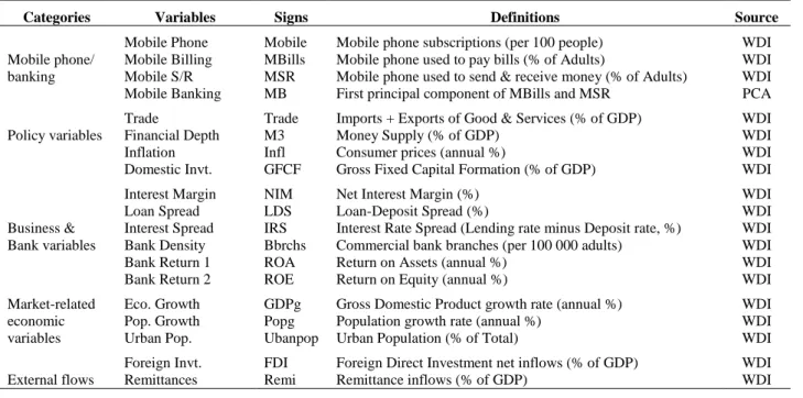
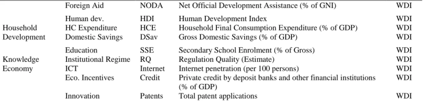
Disclosing the expected signs of the 25 independent variables is not an easy task because of the absence of prior literature that has employed the underlying determinants. Therefore for brevity, we concurrently discuss our intuition for the expected signs with the results. Table 1 and Table 2 present the categorization and definition of variables respectively.
13 Table 1: Mobile phone/banking determinants
Determining Variables Examples
Policy variables (4) Trade policy, macroeconomic policy (Trade, M3, Inflation, GFCF)
Business/Bank variables (6) Investment incentives (NIM, LSD, IRS, Bank density, ROA, ROE)
Market-related economic determinants (3) Market size, market growth, market structure (GDPg, Popg, Ubanpop)
Knowledge Economy (5)
Education (SSE), Institutional Regime (RQ), Innovation (Patents), ICT (Internet), Economic incentives (Private credit).
External Flows (3) FDI, NODA, Remi
Human development (3) HDI, HHCExp, Domestic savings
Source: Authors. M3: Money Supply. GFCF: Gross Fixed Capital Formation. NIM: Net Interest Margin. LSD: Loan Deposit Spread. IRS: Interest Rate Spread. ROA: Return on Assets. ROE: Return on Equity. GDPg: GDP growth. Popg: Population growth. SSE: Secondary School Enrolment. RQ: Regulation Quality. Ubanpop: Urban population. FDI: Foreign Direct Investment. NODA: Net Official Development Assistance. Remi: Remittances. HDI: Human Development Index. HHCExp: Household Consumption Expenditure.
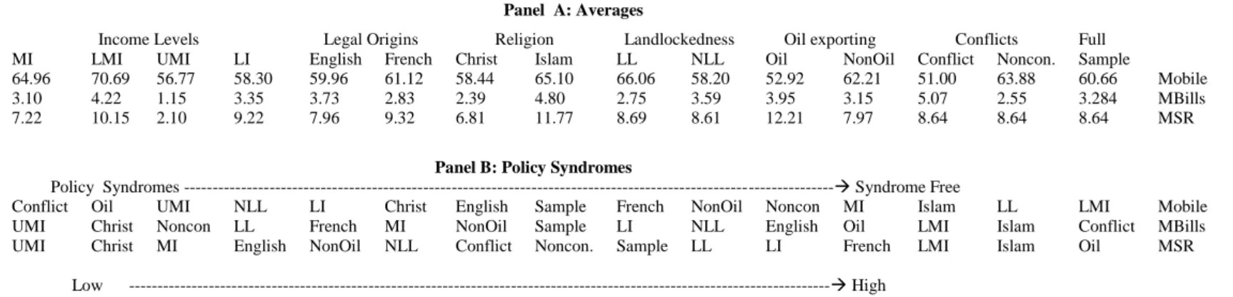
For lack of space, we do not discuss the fundamental characteristics on which the policy syndromes are derived to elaborate detail. The relevant information, which we can provide upon request, is found in a substantial bulk of recent African development literature (Asongu, 2015d). These characteristics are: legal origins (English common law & French civil law), income levels (upper-middle-income, lower-middle-income, middle-income & low-income), conflicts (conflicts & Nonconflicts), oil exports (Oil- & Nonoil-exporting), openness-to-sea (landlocked & unlandlocked) and religious domination (Christianity & Islam).
Table 2: Variable definitions
Categories Variables Signs Definitions Source
Mobile phone/ banking
Mobile Phone Mobile Mobile phone subscriptions (per 100 people) WDI Mobile Billing MBills Mobile phone used to pay bills (% of Adults) WDI Mobile S/R MSR Mobile phone used to send & receive money (% of Adults) WDI Mobile Banking MB First principal component of MBills and MSR PCA Policy variables
Trade Trade Imports + Exports of Good & Services (% of GDP) WDI Financial Depth M3 Money Supply (% of GDP) WDI Inflation Infl Consumer prices (annual %) WDI Domestic Invt. GFCF Gross Fixed Capital Formation (% of GDP) WDI Business &
Bank variables
Interest Margin NIM Net Interest Margin (%) WDI Loan Spread LDS Loan-Deposit Spread (%) WDI Interest Spread IRS Interest Rate Spread (Lending rate minus Deposit rate, %) WDI Bank Density Bbrchs Commercial bank branches (per 100 000 adults) WDI Bank Return 1 ROA Return on Assets (annual %) WDI Bank Return 2 ROE Return on Equity (annual %) WDI Market-related
economic variables
Eco. Growth GDPg Gross Domestic Product growth rate (annual %) WDI Pop. Growth Popg Population growth rate (annual %) WDI Urban Pop. Ubanpop Urban Population (% of Total) WDI External flows
Foreign Invt. FDI Foreign Direct Investment net inflows (% of GDP) WDI Remittances Remi Remittance inflows (% of GDP) WDI
14
Foreign Aid NODA Net Official Development Assistance (% of GNI) WDI Household
Development
Human dev. HDI Human Development Index WDI HC Expenditure HCE Household Final Consumption Expenditure (% of GDP) WDI Domestic Savings DSav Gross Domestic Savings (% of GDP) WDI Knowledge
Economy
Education SSE Secondary School Enrolment (% of Gross) WDI Institutional Regime RQ Regulation Quality (Estimate) WDI ICT Internet Internet penetration (per 100 persons) WDI Eco. Incentives Credit Private credit by deposit banks and other financial institutions
(% of GDP)
WDI Innovation Patents Total patent applications WDI
Eco: Economic. Pop: population. Ivt: Investment. HC: Household Consumption. PCA: Principal Component Analysis. WDI: World Development Indicators of the World Bank. GNI: Gross National Income. S/R: Sending & Receiving.
The summary statistics of the variables is presented in Table 3 below. Two points are worth noting. On the one hand, from mean values, the variables are quite comparable. On the other hand, from the standard deviations, we can be confident that reasonable estimated linkages would emerge due to substantial degrees of variations.
Table 3: Summary statistics
Cross Sectional (2011)
Mean Standard Deviation Minimum Maximum Observations
Mobile Phone 60.66 32.72 4.467 147.2 48 Mobile Billing 3.284 4.97 0.000 26.20 38 Mobile Sending/Receiving 8.644 13.03 0.100 60.50 38 Mobile Banking 0.000 1.279 -0.896 4.505 38 Trade 84.27 33.90 33.28 152.6 46 Financial depth (M3) 36.70 10.84 19.83 53.95 11 Inflation 8.75 8.816 -3.70 47.27 46 Domestic Investment 23.76 9.75 8.80 52.53 42
Net Interest Margin(NIM) 6.009 2.724 2.130 11.36 41
Loan-Deposit Spread (LDS) 11.20 8.651 1.810 41.85 25
Interest Rate Spread (IRS) 11.31 8.579 1.808 41.85 25
Commercial Bank Branches 6.42 8.653 0.626 47.02 43
Return on Assets (ROA) 2.03 0.994 0.25 4.53 41
Return on Equity (ROE) 19.22 8.70 2.85 40.69 41
GDP growth rate (GDPg) 4.585 3.605 -4.728 15.00 47
Population growth (Popg) 2.303 0.852 -0.608 4.156 49
Urban Population (Ubanpop) 38.21 17.51 -1.175 86.14 49
Foreign Direct Investment 7.961 13.26 -2.904 85.36 46
Remittances 4.012 6.018 0.000 26.76 36
Foreign Aid 9.965 10.21 0.211 53.84 47
Human Development Index 0.485 0.103 0.323 0.759 47
Household Expenditure 70.75 21.02 12.26 124.8 39
Domestic Savings 14.65 22.91 -40.15 81.89 42
Secondary School Enrolment 45.78 24.19 14.44 123.8 27
Regulation Quality -0.704 0.648 -2.37 0.849 49
Internet Penetration 10.34 10.42 1.100 43.60 46
Private Domestic Credit 23.84 24.50 5.340 141.4 40
15
Since we are employing 25 independent variables, potential concerns of multicollinearity and overparameterization are mitigated by: (i) using multiple specifications and (ii) avoiding highly correlated variables in the same specification. The substantially correlated variables are highlighted in bold colour in Table 4 or correlation matrix below.
16 Table 4: Correlation matrix
Policy Variables Business/Bank Variables Market-related External Flows Household Development
Knowledge Economy Mobile penetration/banking
Trade M3 Infl. GF CF
NIM LDS IRS Bbr
chs
ROA ROE GDPg Popg UPop FDI Aid Remi HDI HCE DSav SSE RQ Intern
et Credit Paten t Mobil e MBills MSR MB 1.00 0.64 -0.08 0.25 0.00 -0.07 -0.09 0.28 -0.08 -0.05 0.14 -0.37 0.18 0.29 0.05 0.31 0.32 -0.10 0.06 0.46 -0.07 0.20 0.00 -0.11 0.26 0.24 -0.01 0.09 Trade 1.00 -0.35 -0.7 -0.12 1.00 1.00 0.69 -0.19 -0.07 0.20 -0.73 0.85 -0.01 -0.54 0.30 0.78 0.19 -0.04 0.85 0.09 0.64 0.27 0.19 0.69 0.34 -0.03 0.22 M3 1.00 -0.1 0.27 0.29 0.26 -0.1 0.33 0.43 0.10 0.22 -0.27 0.06 0.07 -0.16 -0.16 -0.07 0.05 -0.05 -0.30 0.05 -0.04 -0.05 -0.14 0.24 0.26 0.28 Infl. 1.00 -0.06 -0.24 -0.25 0.2 -0.28 -0.10 0.17 -0.10 -0.09 0.24 0.06 0.08 0.14 -0.18 0.26 0.10 0.21 0.01 -0.05 -0.07 0.18 -0.15 -0.09 -0.12 GFCF 1.00 0.31 0.31 -0.3 0.54 0.21 0.42 0.30 -0.16 0.15 0.34 -0.06 -0.29 0.24 -0.15 -0.32 -0.21 -0.16 -0.36 -0.19 -0.26 -0.01 0.09 0.05 NIM 1.00 0.99 -0.2 -0.04 -0.13 -0.13 0.39 -0.05 0.02 0.28 -0.02 -0.42 0.09 -0.03 -0.33 -0.42 -0.39 -0.39 -0.18 -0.43 -0.25 -0.18 -0.23 LDS 1.00 -0.2 -0.04 -0.13 -0.15 0.40 -0.06 0.01 0.28 -0.02 0.43 0.08 -0.03 -0.33 -0.45 -0.40 -0.40 -0.18 -0.45 -0.27 -0.20 -0.25 IRS 1.00 -0.28 -0.25 0.09 -0.69 0.13 -0.01 -0.08 -0.00 0.67 -0.06 0.03 0.90 0.37 0.77 0.40 0.07 0.54 0.26 0.08 0.17 Bbrchs 1.00 0.73 0.17 0.10 -0.39 -0.02 0.08 -0.04 -0.22 0.33 -0.43 -0.34 -0.05 -0.16 -0.16 -0.15 -0.24 0.12 0.08 0.11 ROA 1.00 0.16 0.02 -0.18 0.07 -0.08 0.04 -0.18 0.16 -0.25 -0.30 -0.09 -0.26 -0.16 -0.06 -0.07 -0.05 -0.13 -0.10 ROE 1.00 -0.04 0.00 0.22 0.20 -0.04 0.11 0.13 -0.11 0.12 0.01 0.01 -0.02 -0.04 0.13 -0.06 -0.16 -0.13 GDPg 1.00 -0.24 0.14 0.23 -0.03 -0.61 -0.11 0.12 -0.81 -0.27 -0.55 -0.46 -0.19 -0.38 -0.03 -0.06 -0.05 Popg 1.00 0.11 -0.17 -0.03 0.39 -0.22 0.32 0.20 0.12 0.08 0.07 0.19 0.54 0.08 0.12 0.11 UPop 1.00 0.61 0.49 -0.15 0.33 -0.27 0.001 -0.13 -0.13 -0.12 -0.07 -0.09 -0.001 -0.08 -0.05 FDI 1.00 0.40 -0.45 0.55 -0.53 -0.18 -0.18 -0.29 -0.11 -0.14 -0.46 -0.12 -0.20 -0.18 Aid 1.00 -0.12 0.66 -0.73 0.04 -0.15 -0.06 -0.13 -0.10 -0.13 0.10 0.001 0.04 Remi 1.00 -0.42 0.40 0.91 0.54 0.71 0.51 0.23 0.81 0.26 0.32 0.35 HDI 1.00 -0.96 -0.04 0.00 -0.16 -0.03 -0.08 -0.48 0.00 -0.06 -0.03 HCE 1.00 -0.00 -0.01 0.12 -0.07 0.02 0.47 -0.02 0.18 0.11 DSav 1.00 0.42 0.89 0.60 0.00 0.64 0.08 0.36 0.21 SSE 1.00 0.38 0.61 0.25 0.48 -0.31 -0.07 -0.21 RQ 1.00 0.51 0.15 0.41 0.15 0.42 0.32 Internet 1.00 0.77 0.44 0.15 0.02 0.08 Credit 1.00 0.36 0.03 -0.04 -0.00 Patent 1.00 -0.08 0.15 0.03 Mobile 1.00 0.63 0.90 MBills 1.00 0.90 MSR 1.00 MB
M3: Money Supply. Infl: Inflation. GFCF: Gross Fixed Capital Formation. NIM: Net Interest Margin. LDS: Lending Deposit Spread. IRS: Interest Rate Spread. Bbrchs: Bank Branches. ROA: Return on Assets. ROE: Return on Equity. GDPg: GDP growth. Popg: Population growth. UPop: Urban population. FDI: Foreign Direct Investment. Aid: Net Official Development Assistance. Remi: Remittance. HDI: Human Development Index. HCE: Household consumption expenditure. DSav: Domestic savings. SSE: Secondary School Enrolment. RQ: Regulation Quality. Internet: internet penetration. Credit: Private Domestic Credit. Patent: Total patent applications. Mobile: Mobile phone penetration. MBills: Mobile phone used to pay bills. MSR: Mobile phone used to send and receive money. MB: Mobile Banking. Potential issues of multicollinearity highlighted in bold colour.
17 3.2 Methodology
3.2.1 Principal component analysis (PCA)
We use PCA because we aim to reduce the observed correlated variables into a smaller set of independent and/or uncorrelated composite variables. In other words, we wish to extract linear composites of observed variables. Factor analysis is inappropriate because we are not testing a theoretical model of latent factors causing observed variables. Accordingly, it is consistent with the test for a theoretical model of latent factors causing observed variables.
The interest of employing the PCA technique to obtain a composite mobile banking indicator is therefore twofold. On the one hand, the two mobile indicators for (i) paying bills and (ii) receiving/sending money are potentially highly correlated, since the same mobile phone may be used to send/receive money and pay bills. On the other hand, we need a mobile banking indicator for a conceptual justification. The PCA is a widely employed technique in econometrics that is used to reduce a set of highly correlated variables into a smaller set of uncorrelated variables called principal components (PCs).
The criteria we use to retain the common mobile banking factor is from Kaiser (1974) and Jolliffe (2002) who have recommended that we stop at PCs with eigenvalues that are greater than one (or higher than the mean). As shown in Table 5 below, the first PC (or mobile banking indicator) has an eigenvalue of 1.636 and represents more than 81% of combined information or variability in the constituent indicators.
Table 5: Principal Component Analysis for the Mobile banking composite indicator
Principal Components
Component Matrix (Loadings) Proportion Cumulative Proportion
Eigen Value MBills MSend/Rec
First PC 0.707 0.707 0.818 0.818 1.636
Second PC -0.707 0.707 0.181 1.000 0.363
PC: Principal Component. MBill: Mobile phone used to pay bills. MSendRec: Mobile phone used to Send and Receive money.
Consistent with Asongu and Nwachukwu (2016) there are concerns with factor- augmented variables or indicators obtained from underlying or first-stage regressions. Three of such issues have been raised by Pagan (1984, p. 242) in relation to estimated parameters. These include: (i) consistency, (ii) efficiency and, (iii) validity of inferences obtained from the latter-stage estimations. The author established that while estimated parameters from a two-step procedure are efficient and consistent, inferences are not always valid. These concerns have been abundantly discussed in a recent current of the literature, inter alia: Oxley and
18
McAleer (1993), Ba and Ng (2006), McKenzie and McAleer (1997) and Westerlund and Urbain (2013a).
In this study we employ a mobile banking PC. To the best of our knowledge, concerns about inferences related to PC loadings have been documented by Westerlund and Urbain (2012, 2013b). Building on previous studies (Greenaway-McGrevy et al., 2012; Bai, 2009; Pesaran, 2006; Bai, 2003; Stock & Watson, 2002), they conclude that normal inferences are feasible with augmented regressions from PC-factors as long as the estimated coefficients
converge towards their true values at the following rate: NT (with T being the number of periods in a time series and N, the number of agents or cross sections). While the authors have further postulated that N and T should be sufficiently large, they have not clearly articulated the magnitude of the largeness. We argue that our N and T do not constraint the analysis with issues of small sample bias for the following reasons. First, on the N constraint, the exposition is based on sub-Saharan African countries and all 49 countries in the underlying region are covered in the study. Second, with respect to the constraint on T, mobile banking indicators are only available for the year 2011. Moreover, Asongu and Nwachukwu (2015) have recently shown that in the presence of a high degree of correlation between the PC-augmented variable and constituent indicators, the resulting inferences are not significantly different.
3.2.2 Estimation technique
Consistent with the motivation of the study, in order to assess why some countries are more successful in mobile phone/banking activities, we employ an estimation technique that distinguishes countries in terms mobile phone/banking penetration rates. Hence, the quantile regression (QR) technique is adapted to the problem statement because it enables us to assess the determinants of mobile phone/banking penetration throughout the conditional distributions of the determinants. In this light, countries in low (high) quantiles are considered as least (best) performing in the underlying dependent variables.
Following Keonker and Hallock (2001), the QR technique is being increasingly utilized to assess multiple points in the distribution of development outcomes, inter alia in: corruption (Billger & Goel, 2009; Okada & Samreth, 2012) and financial development (Asongu, 2014a) studies. The proposed technique has also been recently applied on cross-sectional data (Asongu, 2014b).
In accordance with the empirical underpinnings, the th quantile estimator of the dependent variable is obtained by estimating Eq. (1) below.
19
i i i i i i k x y i i i x y i i i R x y x y : : ) 1 ( min (1)Where ∈ (0,1). Contrary to Ordinary Least Squares (OLS), which minimizes the sum of squared residuals, the approach in Eq. (1) consists of minimizing the weighted sum of absolute deviations. In this technique, the 10th or 90th quantiles (=0.10 or 0.90 respectively) are obtained by approximately weighing residuals.
The conditional quantile of dependent variables (yi) given the determinants (xi) is:
i i y x x
Q ( / ) (2)
where unique slope parameters are estimated for each th quantile (mobile phone penetration/ mobile banking or composite indicator). This formulation is analogous to
i
x x y
E( / ) in the slope from OLS though parameters are modeled only at the mean of conditional distributions of the mobile phone/banking variables.
4. Empirical results
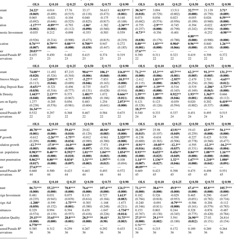
This section presents the empirical findings which are divided into two sub-sections. While Section 4.1 presents mobile phone determinants (Table 6), mobile banking determinants are covered in Section 4.2, notably for: ‘mobile for bills payment’ (Table 7), ‘mobile for receiving/sending money’ (Table 8) and the composite indicator or ‘mobile banking’ (Table 9). We present each of the tables in six different specifications to avoid issues of multicollinearity and overparameterization highlighted in Table 4. This specification strategy is consistent with the highlighted empirical underpinnings (see Billger & Goel, 2009). The Left-Hand-Side (LHS) and Right-Hand-Side (RHS) denote contemporary and non-contemporary specifications respectively.
From a general perspective, we notice that for the most part, the corresponding OLS specifications do not have valid information criteria, notably: negative adjustment coefficients and insignificant Fisher statistics used to assess the overall significance of models. We extend the OLS modelling with alternative specifications and find that, but for the modelling of ‘OLS mobile phone determinants’ in Appendix 1 for which the information criteria validates the significance of the underlying OLS models, OLS is not a good fit for modelling determinants of ‘mobile usage for paying bills’ (Appendix 2), ‘mobile usage for sending/receiving money’
20
(Appendix 3) and ‘mobile usage for banking’ (Appendix 4). In light of the above, the quantile regression estimations are preferred because baseline OLS models are not good fits. When interpreting the quantile regression estimates, it should be noted that low quantiles correspond to dependent variables with the lower mobile phone/banking penetration rates.
4.1 Conditional mobile phone determinants
Table 6 presents conditional mobile phone penetration determinants. Differences in patterns, signs and ‘magnitude of significance’ between the OLS and QR estimations justify the need for using the latter approach to provide more robust estimations. The following can be established from the findings. First, mobile phone penetration is: (1) negatively correlated with inflation with the effects more apparent in the lowest (0.10th) and highest (0.90th) quantiles; (2) negatively correlated with domestic investment in the middle (0.50th) of the non-contemporary specification and (3) positively linked to education with more significance in the bottom quantiles of the distributions.
Second: (1) the relationship with Net Interest Margin (NIM) is not clear-cut because a bottom (top) quantile is positively (negatively) linked to the dependent variables; (2) the lending-deposit-rate is negatively correlated, with the nexus most apparent in bottom and top quantiles of non-contemporary specifications; (3) bank density is significantly positively correlated throughout the distributions, but for the 0.90th (0.25th & 0.75th) quantile (s) in non-contemporary (non-contemporary) specifications and (4) Return on Equity (ROE) is positively correlated only in one (0.90th) of the top quantiles.
Third: (1) GDP is only significant in the LHS, with mixed signs or a negative nexus in bottom quantiles (0.10th & 0.25th) and a positive relationship in a top quantile (0.90th); (2) but for the 0.75th (0.50th) quantile in the LHS (RHS), population growth consistently exhibits a negative sign; (3) there is a threshold correlation with positive increasing magnitudes in the LHS (RHS) throughout the distribution (from the 0.25th to the 0.90th quantile) in urban population and (4) there is also threshold positive evidence in internet penetration from the 0.25th to the 0.75th quantile in the LHS and RHS.
Fourth: (1) the positive correlation of FDI is apparent only in the 0.90th quantile of the LHS; (2) foreign aid is negatively correlated only in bottom quantiles; (3) the negative nexus of remittances is only apparent in the 0.90th quantile of the LHS; (4) the positive relationship of regulation quality is consistently significant in the LHS and sparsely significant in the RHS (0.10th & 0.50th); (5) while the effect of human development is consistently significant across
21
specifications in the LHS and RHS; (6) domestic savings, regulation quality and patent applications are only significant in the bottom quantiles of the LHS and (7) the relationship of private credit is mixed, with negative and positive signs respectively in the 0.10th and 0.50th quantiles of the LHS and a positive sign in the RHS (0.25th quantile).
Table 6: Conditional determinants of Mobile phone penetration
Contemporary Non-contemporary OLS Q 0.10 Q 0.25 Q 0.50 Q 0.75 Q 0.90 OLS Q 0.10 Q 0.25 Q 0.50 Q 0.75 Q 0.90 Constant 24.22* 4.014 17.76 33.17 56.613 61.93*** 30.34** 3.094 13.511 32.7*** 21.139 3.71* (0.069) (0.489) (0.515) (0.118) (0.473) (0.001) (0.018) (0.729) (0.802) (0.000) (0.750) (0.089) Trade 0.065 -0.021 -0.104 0.040 -0.175 0.140 0.071 0.036 0.023 -0.055 0.026 0.59*** (0.692) (0.646) (0.525) (0.825) (0.817) (0.168) (0.682) (0.574) (0.956) (0.189) (0.960) (0.000) Inflation -1.17*** -0.89*** -0.793 -1.06* -1.382 -2.34*** -0.755 -2.9*** -0.745 -0.394 -0.022 -0.93*** (0.002) (0.001) (0.112) (0.090) (0.560) (0.000) (0.257) (0.000) (0.798) (0.242) (0.994) (0.000) Domestic Investment -0.035 0.212 -0.098 -0.353 -0.503 0.559 -0.73** -0.356 -0.401 -0.80*** -0.252 -0.98*** (0.926) (0.214) (0.900) (0.473) (0.815) (0.219) (0.038) (0.179) (0.788) (0.000) (0.900) (0.000) Education 0.76*** 0.79*** 0.88*** 0.708** 0.947 0.272 0.80*** 1.03*** 0.904* 0.96*** 0.840 1.26*** (0.007) (0.000) (0.000) (0.030) (0.447) (0.185) (0.001) (0.000) (0.066) (0.000) (0.308) (0.000) Fisher 20.03*** --- --- --- --- --- 17.6*** --- --- --- --- --- Adjusted/Pseudo R² 0.435 0.450 0.402 0.415 0.374 0.319 0.390 0.311 0.323 0.419 0.398 0.372 Observations 23 23 23 23 23 23 22 22 22 22 22 22 OLS Q 0.10 Q 0.25 Q 0.50 Q 0.75 Q 0.90 OLS Q 0.10 Q 0.25 Q 0.50 Q 0.75 Q 0.90 Constant 74.08** 11.492 87.215 90.6*** 106.1* 116.0*** 71.2*** 15.3*** 65.7*** 62.3*** 91.3*** 131.2*** (0.028) (0.324) (0.344) (0.006) (0.060) (0.000) (0.000) (0.006) (0.001) (0.005) (0.005) (0.000)
Net Interest Margin -5.445 2.091** -4.757 -5.27** -7.853 -10.5*** -2.412 1.83*** -2.957* -2.479 2.703 -4.65**
(0.113) (0.044) (0.689) (0.046) (0.163) (0.000) (0.115) (0.000) (0.067) (0.254) (0.286) (0.012)
Lending Deposit Rate -0.651** -0.321 -0.496 -0.735 -0.673 -0.037 -0.88*** -1.19*** -0.516 -0.519 -1.206* -1.73***
(0.038) (0.316) (0.777) (0.131) (0.628) (0.916) (0.001) (0.000) (0.165) (0.169) (0.063) (0.000) Bank Density 1.443** 2.13*** 0.375 1.481** 1.072 0.666** 1.59*** 1.89*** 0.922** 1.93*** 1.365** 0.666 (0.040) (0.000) (0.867) (0.015) (0.186) (0.011) (0.020) (0.000) (0.046) (0.001) (0.026) (0.112) Return on Equity 1.277 -0.205 0.056 0.483 1.254 2.073*** 0.121 0.123 -0.039 0.020 0.202 0.419*** (0.238) (0.576) (0.981) (0.604) (0.641) (0.000) (0.328) (0.126) (0.594) (0.882) (0.337) (0.000) Fisher 16.34*** --- --- --- --- --- 18.3*** --- --- --- --- --- Adjusted/Pseudo R² 0.532 0.297 0.368 0.467 0.584 0.675 0.540 0.333 0.337 0.451 0.495 0.515 Observations 22 22 22 22 22 22 24 24 24 24 24 24 OLS Q 0.10 Q 0.25 Q 0.50 Q 0.75 Q 0.90 OLS Q 0.10 Q 0.25 Q 0.50 Q 0.75 Q 0.90 Constant 48.78*** 66.3*** 59.41** 29.82 40.94* 84.80*** 31.35** 25.98 43.91** 19.43 43.9*** 56.1*** (0.001) (0.000) (0.010) (0.129) (0.085) (0.000) (0.015) (0.107) (0.049) (0.259) (0.008) (0.000) GDP growth -0.612 -2.26*** -1.75** -0.012 -0.961 2.325*** -0.238 -0.634 -0.590 -0.227 0.425 0.530 (0.209) (0.000) (0.034) (0.989) (0.380) (0.000) (0.600) (0.383) (0.506) (0.778) (0.560) (0.477) Population growth -12.7*** -17.9*** -16.0*** -8.689* -7.971 -19.8*** -8.91** -10.05** -12.3** -4.595 -12.3** -16.2*** (0.005) (0.000) (0.000) (0.097) (0.334) (0.000) (0.016) (0.021) (0.037) (0.331) (0.016) (0.004) Urban population 0.983*** 0.48*** 0.592** 1.01*** 1.04*** 1.054*** 0.93*** 0.655** 0.456** 0.84*** 1.08*** 1.16*** (0.000) (0.000) (0.018) (0.000) (0.003) (0.000) (0.000) (0.025) (0.049) (0.000) (0.000) (0.000) Internet penetration 0.862** 0.80*** 0.834* 1.31*** 1.597** 0.108 1.14*** 1.136** 1.32** 1.67*** 1.210** 1.080* (0.017) (0.000) (0.097) (0.003) (0.015) (0.694) (0.007) (0.027) (0.046) (0.000) (0.041) (0.091) Fisher 27.63*** --- --- --- --- --- 40.09*** --- --- --- --- --- Adjusted/Pseudo R² 0.660 0.500 0.423 0.463 0.493 0.572 0.669 0.423 0.398 0.475 0.498 0.551 Observations 44 44 44 44 44 44 45 45 45 45 45 45 OLS Q 0.10 Q 0.25 Q 0.50 Q 0.75 Q 0.90 OLS Q 0.10 Q 0.25 Q 0.50 Q 0.75 Q 0.90 Contant 86.71*** 55.23*** 78.8*** 76.6*** 107.6*** 124.5*** 71.1*** 38.6*** 49.9*** 67.4*** 85.8*** 105.7*** (0.000) (0.000) (0.000) (0.000) (0.000) (0.000) (0.000) (0.000) (0.000) (0.000) (0.000) (0.000) Foreign Investment 0.481 0.031 0.075 0.115 0.727 1.613* 0.182 0.326 -0.029 0.465 0.290 -0.647 (0.235) (0.943) (0.839) (0.614) (0.184) (0.083) (0.784) (0.818) (0.953) (0.651) (0.782) (0.716) Foreign Aid -1.208* -0.599 -1.75*** -0.303 -1.168 -1.673 -0.240 -0.091 -0.79*** -0.586 -0.204 -0.112 (0.050) (0.152) (0.001) (0.380) (0.248) (0.211) (0.346) (0.811) (0.000) (0.161) (0.579) (0.783) Remittances 0.329 0.994 0.394 0.439 -1.047 -1.734** 0.153 0.803 0.244 0.328 -0.876 -0.487 (0.574) (0.119) (0.557) (0.418) (0.226) (0.014) (0.767) (0.130) (0.345) (0.775) (0.420) (0.784) Regulation Quality 29.15*** 33.65*** 28.8*** 28.5*** 30.41* 31.75*** 27.5*** 29.1*** 5.591 26.90** 27.03 26.814 (0.000) (0.000) (0.001) (0.000) (0.98) (0.003) (0.000) (0.002) (0.180) (0.012) (0.151) (0.154) Fisher 6.778*** --- --- --- --- --- 6.56*** --- --- --- --- --- Adjusted/Pseudo R² 0.385 0.312 0.259 0.267 0.292 0.433 0.226 0.215 0.172 0.189 0.269 0.264 Observations 36 36 36 36 36 36 36 36 36 36 36 36
22 OLS Q 0.10 Q 0.25 Q 0.50 Q 0.75 Q 0.90 OLS Q 0.10 Q 0.25 Q 0.50 Q 0.75 Q 0.90 Constant -33.93* -34.05* -7.423 -27.27 -54.44 -27.37 -43.4*** -43.03 -20.20 -33.69 -57.03* -49.37 (0.077) (0.099) (0.719) (0.177) (0.288) (0.419) (0.007) (0.224) (0.479) (0.142) (0.058) (0.234) Human Development 203.8*** 162.2*** 122.8*** 185.7*** 263.0*** 245.9*** 206.5*** 172*** 140*** 189*** 259*** 245*** (0.000) (0.000) (0.001) (0.000) (0.008) (0.000) (0.000) (0.006) (0.007) (0.000) (0.000) (0.000) Domestic Savings 0.063 0.210** 0.214** -0.109 0.051 -0.031 0.019 -0.061 0.093 -0.074 -0.143 0.072 (0.624) (0.015) (0.033) (0.421) (0.858) (0.814) (0.861) (0.673) (0.621) (0.663) (0.440) (0.706) Regulation Quality 6.146 10.32** 14.17** 5.473 0.080 9.00 2.684 8.078 6.844 3.960 0.917 0.706 (0.355) (0.012) (0.048) (0.356) (0.996) (0.353) (0.624) (0.220) (0.510) (0.551 (0.909) (0.953) Patent Applications 0.003*** 0.006*** 0.006*** 0.004*** 0.001 -0.001 0.001* 0.005*** 0.004*** 0.002* -0.0008 -0.001 (0.003) (0.000) (0.000) (0.000) (0.514) (0.416) (0.089) (0.000) (0.002) (0.071) (0.580) (0.549) Fisher 201.4*** --- --- --- --- --- 125.2*** --- --- --- --- --- Adjusted/Pseudo R² 0.664 0.487 0.449 0.440 0.479 0.566 0.661 0.434 0.435 0.471 0.518 0.473 Observations 41 41 41 41 41 41 41 41 41 41 41 41 OLS Q 0.10 Q 0.25 Q 0.50 Q 0.75 Q 0.90 OLS Q 0.10 Q 0.25 Q 0.50 Q 0.75 Q 0.90 Constant -7.183 -27.82 -29.56 -19.73 -46.08 1.246 -43.00** -75.41** -39.44 -36.61 -43.58 -140*** (0.772) (0.256) (0.420) (0.570) (0.573) (0.976) (0.024) (0.023) (0.117) (0.124) (0.514) (0.000) Human Development 169*** 181.6*** 158.2** 162.5*** 252.5* 209*** 196.6*** 193.6*** 137*** 177*** 246** 342.2*** (0.000) (0.000) (0.012) (0.003) (0.067) (0.001) (0.000) (0.000) (0.000) (0.000) (0.025) (0.000) Household expenditure -0.110 -0.082 0.143 0.008 -0.077 -0.140 0.072 0.267** 0.100 0.078 -0.081 0.807*** (0.467) (0.373) (0.349) (0.963) (0.811) (0.586) (0.511) (0.037) (0.438) (0.488) (0.796) (0.000) Regulation Quality 10.98 10.89** 5.540 9.606 -1.303 15.984 2.357 -2.251 -6.664 4.951 2.933 -6.846 (0.199) (0.011) (0.549) (0.298) (0.959) (0.411) (0.718) (0.682) (0.266) (0.429) (0.878) (0.263) Private Credit 0.058 -0.145* -0.043 0.260** 0.103 -0.055 0.020 0.059 0.335*** 0.123 -0.064 -0.152 (0.287) (0.094) (0.775) (0.035) (0.806) (0.834) (0.875) (0.451) (0.000) (0.144) (0.717) (0.129) Fisher 9.486*** --- --- --- --- --- 14.99*** --- --- --- --- --- Adjusted/Pseudo R² 0.651 0.487 0.474 0.467 0.464 0.543 0.628 0.476 0.471 0.490 0.476 0.426 Observations 32 32 32 32 32 32 34 34 34 34 34 34
Notes. Dependent variable is Mobile Phone Penetration. *,**,***, denote significance levels of 10%, 5% and 1% respectively. Lower quantiles (e.g., Q 0.1) signify nations where the Mobile Phone Penetration is least. OLS: Ordinary Least Squares. In some specifications, non-contemporary observations may exceed contemporary-observations if there are missing observations in the latter.
4.2 Conditional Mobile Banking Determinants
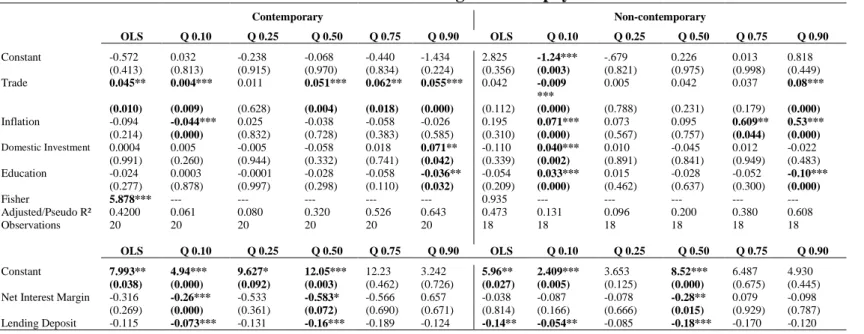
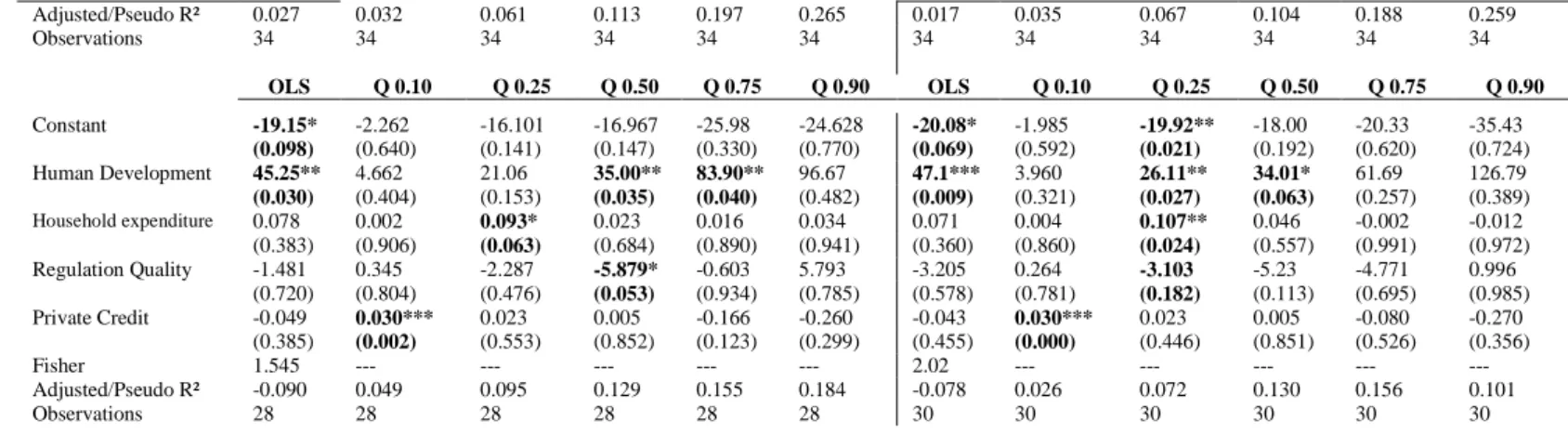
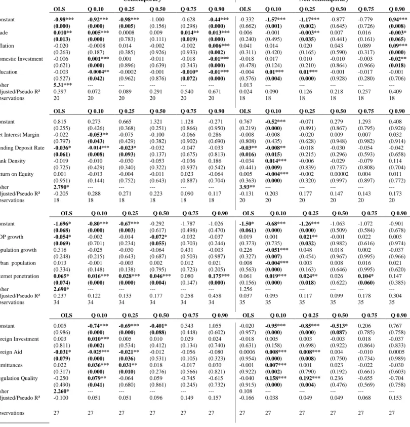
This section presents the findings of conditional determinants of mobile banking, composed of the use of mobile phones to: (i) pay bills and (ii) receive/send money. The following findings can be established for Table 7 on mobiles used to pay bills. First: (1) while the correlation with trade is mixed in the RHS with negative and positive signs in the a bottom (0.10th) and a top (0.90th) quantile, but for the 0.25th, it is consistently positive throughout the distribution on the LHS; (2) the nexus with inflation is also mixed, with positive relationships in a bottom (0.10th) quantile and top (0.75th & 0.90th) quantiles in the RHS, it is negatively linked to the dependent variable in a bottom (0.10th) quantile of the LHS; (3) the correlation with domestic investment is only in a top or 0.90th (bottom or 0.10th ) quantile of the RHS (LHS); (4) the relationship with education is mixed, with a negative sign in the 0.90th quantile of both contemporary and non-contemporary specifications and only a positive in the 0.10th quantile of the latter specification; (5) the relationships of NIM, lending-deposit-rate and bank density are consistently negative in the 0.10th and 0.50th in LHS and in the 0.50th quantile of the RHS and (6) in the RHS, the nexus with the dependent variable is negative for the lending-deposit-rate in the 0.10th quantile and positive for ROE in the 0.50th quantile.
23
Second: (1) while but for the 0.75th quantile, the relationship with internet penetration is consistently positive in the LHS, it is only positive in bottom (0.25th) and top (0.90th) on the RHS; (2) the nexus of growth is negative in a top (0.90th) quantile and positive in a bottom (0.10th) quantile in the LHS and RHS respectively; (3) the nexus with population is only significantly negative in a bottom (0.10th) of the LHS; (4) the relationship with urban population is positive in a top (0.90th) quantile in both the LHS and RHS and only significantly negative in the 0.10th quantile of the RHS.
Third: (1) the nexus with FDI is positive in bottom quantiles of the LHS and negative only in a top (0.90th) quantile of the RHS; (2) while the nexus with foreign aid is negative in a bottom (0.25th) quantile and a top (0.90th) quantile in the LHS while, in the RHS, it is positive in the bottom quantiles and a top (0.90th) quantile; (3) the relationship with remittances is positive in the bottom-half of the LHS and only in a bottom (0.10th) quantile of the RHS and; (4) regulation quality is positively significant only in the bottom quantiles, at the 0.10th quantile of the LHS and 0.10th and 0.25th quantiles of the RHS.
Fourth: (1) human development is positively significant in the bottom-halves of the distribution and only in the 0.90th quantile of the RHS; (2) domestic savings are only negatively significant in the 0.25th of the LHS and RHS; (3) ‘patent applications’ is positively significant in the bottom-halves of the distribution and only negative in the 0.90th of the RHS; (4) household expenditure (regulation quality) is negative only in the 0.10th (0.90th) quantile of the RHS (LHS), while the positive effect of private credit is only significant in the bottom quantiles of the RHS.
Table 7: Conditional determinants of Mobile usage for Bills payment
Contemporary Non-contemporary OLS Q 0.10 Q 0.25 Q 0.50 Q 0.75 Q 0.90 OLS Q 0.10 Q 0.25 Q 0.50 Q 0.75 Q 0.90 Constant -0.572 0.032 -0.238 -0.068 -0.440 -1.434 2.825 -1.24*** -.679 0.226 0.013 0.818 (0.413) (0.813) (0.915) (0.970) (0.834) (0.224) (0.356) (0.003) (0.821) (0.975) (0.998) (0.449) Trade 0.045** 0.004*** 0.011 0.051*** 0.062** 0.055*** 0.042 -0.009 *** 0.005 0.042 0.037 0.08*** (0.010) (0.009) (0.628) (0.004) (0.018) (0.000) (0.112) (0.000) (0.788) (0.231) (0.179) (0.000) Inflation -0.094 -0.044*** 0.025 -0.038 -0.058 -0.026 0.195 0.071*** 0.073 0.095 0.609** 0.53*** (0.214) (0.000) (0.832) (0.728) (0.383) (0.585) (0.310) (0.000) (0.567) (0.757) (0.044) (0.000) Domestic Investment 0.0004 0.005 -0.005 -0.058 0.018 0.071** -0.110 0.040*** 0.010 -0.045 0.012 -0.022 (0.991) (0.260) (0.944) (0.332) (0.741) (0.042) (0.339) (0.002) (0.891) (0.841) (0.949) (0.483) Education -0.024 0.0003 -0.0001 -0.028 -0.058 -0.036** -0.054 0.033*** 0.015 -0.028 -0.052 -0.10*** (0.277) (0.878) (0.997) (0.298) (0.110) (0.032) (0.209) (0.000) (0.462) (0.637) (0.300) (0.000) Fisher 5.878*** --- --- --- --- --- 0.935 --- --- --- --- --- Adjusted/Pseudo R² 0.4200 0.061 0.080 0.320 0.526 0.643 0.473 0.131 0.096 0.200 0.380 0.608 Observations 20 20 20 20 20 20 18 18 18 18 18 18 OLS Q 0.10 Q 0.25 Q 0.50 Q 0.75 Q 0.90 OLS Q 0.10 Q 0.25 Q 0.50 Q 0.75 Q 0.90 Constant 7.993** 4.94*** 9.627* 12.05*** 12.23 3.242 5.96** 2.409*** 3.653 8.52*** 6.487 4.930 (0.038) (0.000) (0.092) (0.003) (0.462) (0.726) (0.027) (0.005) (0.125) (0.000) (0.675) (0.445)
Net Interest Margin -0.316 -0.26*** -0.533 -0.583* -0.566 0.657 -0.038 -0.087 -0.078 -0.28** 0.079 -0.098
(0.269) (0.000) (0.361) (0.072) (0.690) (0.671) (0.814) (0.166) (0.666) (0.015) (0.929) (0.787)