The impact of oil price shocks on the stock market return and
volatility relationship
Wensheng Kang
a,*, Ronald A. Ratti
b, Kyung Hwan Yoon
ba
Department of Economics, Kent State University, OH, USA b
School of Business, University of Western Sydney, NSW, Australia
A R T I C L E I N F O
Article history:
Received 20 September 2014 Accepted 2 November 2014 Available online 6 November 2014
JEL classifications:
E44 G10 Q41 Q43
Keywords:
Stock return and volatility Oil price shocks Stock volatility Structural VAR
A B S T R A C T
This paper examines the impact of structural oil price shocks on the covariance of U.S. stock market return and stock market volatility. We construct from daily data on return and volatility the covariance of return and volatility at monthly frequency. The measures of daily volatility are realized-volatility at high frequency (normalized squared return), conditional-volatility recovered from a stochastic volatility model, and implied-volatility deduced from options prices. Positive shocks to aggregate demand and to oil-market specific demand are associated with negative effects on the covariance of return and volatility. Oil supply disruptions are associated with positive effects on the covariance of return and volatility. The spillover index between the structural oil price shocks and covariance of stock return and volatility is large and highly statistically significant.
ã2014 Elsevier B.V. All rights reserved.
1. Introduction
A considerable volume of work has emerged examining the connections between oil price shocks and stock returns and between oil price shocks and stock market volatility. Early papersfinding a negative relationship between oil prices and stock market returns includeJones and Kaul (1996), for Canada and the U.S.,Sadorsky (1999)for the U.S., andPapapetrou (2001)for Greece.Nandha and Faff (2008)report a negative connection between oil prices and global industry indices,Chen (2010)establishes that an increase in oil prices leads to a higher probability of a declining S&P index, andMiller and Ratti (2009)find that stock market indices in 6 OECD countries respond negatively to increases in the oil price in the long run, particularly before 2000.1In an important contribution,Kilian and Park (2009)emphasize that in analyzing the influence of oil prices on the stock market, it is essential to identify the underlying source of the oil price shocks.Kilian and Park (2009)
* Corresponding author. Tel.: +1 330 308 7414.
E-mail address:wkang3@kent.edu(W. Kang).
1
A negative effect of positive oil price shocks on stock market return has been confirmed by a number of authors for oil importing countries.
Jimenez-Rodriguez and Sanchez (2005)argue that the negative effects for oil importing countries are reinforced because of intensive trade connections.
Arouri and Rault (2011)find that large oil price changes have a positive impact on stock returns in oil-exporting countries.
http://dx.doi.org/10.1016/j.intfin.2014.11.002
1042-4431/ã2014 Elsevier B.V. All rights reserved.
Int. Fin. Markets, Inst. and Money 34 (2015) 41–54
Contents lists available atScienceDirect
Journal of International Financial
Markets, Institutions & Money
j o u r n a l h o m e p a g e : w w w . e l s e v i e r . c o m / l o c a t e / i n t fi nshow that oil price increases driven by aggregate demand cause U.S. stock markets to rise and that those driven by oil-market specific demand shocks cause stock markets to fall.2
With regard to the effect of oil price shocks on stock market volatility,Malik and Ewing (2009)find evidence of significant transmission of volatility between oil and some sectors in the US stock market,Vo (2011)shows that there is inter-market dependence in volatility between U.S. stock and oil markets, and Arouri et al. (2012) report that there is volatility transmission from oil to European stock markets.Degiannakis et al. (2014)show that a rise in price of oil associated with increased aggregate demand significantly raises stock market volatility in Europe, and that supply-side shocks and oil specific demand shocks do not affect volatility.
The objective in this paper is to investigate how structural oil price shocks drive the contemporaneous stock market return and volatility relationship. In recent years, there has been considerable volatility in the U.S. stock market and dramatic fluctuation in the global price for crude oil. The relationship between stock market return and volatility is of central importance infinance. Under the capital asset pricing model ofMerton (1980), return and volatility of the aggregate stock market portfolio are positively related, although empricial confirmation of the nature of relationship has been controversial.3 Bollerslev and Zhou (2006) put much of the diversity of findings about the stock market return and volatility relationship down to different methods of measuring volatility. The measures of volatility used in empirical examination of the links between stock return and volatility have included realized-volatility, based on using high frequency data to compute measures of volatility at a lower frequency, conditional-volatility, recovered from a stochastic volatility model, and implied-volatility, deduced from options prices.
In this paper, we will construct from daily data of return and volatility the covariance of return and volatility at monthly frequency. The measures of daily volatility are realized-volatility at high frequency (normalized squared return), conditional-volatility recovered from a stochastic conditional-volatility model, and implied-conditional-volatility deduced from options prices. The latter variable provides a forward looking measure of the contemporaneous stock market return and volatility relationship.
It is found that a positive shock to aggregate demand is associated with negative effects on the covariances of return and volatility with the statistical significance of the effect extending for a longer period for implied-covariance. Positive shocks to oil-market specific demand have a statistically significant negative effect on the return and volatility covariance relationships over thefirst four tofive months of the shock. In contrast to thefindings for realized or conditional-covariance, an unanticipated reduction in crude oil production is associated with a statistically significant increase in implied-covariance of return and volatility that extends for 24 months. In the long-term, shocks to global oil supply, innovations in aggregate demand, and oil-market specific demand disturbances forecast 14.7%,13.7%, and 33% of the variation in the stock market implied-covariance of return and volatility.
To investigate the changes in the dynamics of oil price shocks and the covariance in U.S. stock market return and volatility over time, we estimate a structural vector autoregression (SVAR) model using rolling samples. The fraction of the variation of implied-covariance of return and volatility explained by oil-market specific demand shocks increased dramatically in 2008:09 to around 43%, and has averaged over 40% since that time. Global oil production predicts 8.4% of the variance of implied-covariance of return and volatility over 2005–2006 before rising to an average of 21.3% from March to September in 2008, and averaging 18.6% over 2011:07–2013:12. This contrasts with the contribution of global aggregate demand to forecasting the implied-covariance of return and volatility which is greater over 2005–2006 (about 30.0%) than subsequently, (11.5% over 2011:01–2013:12).
The paper is organized as follows. Section2describes the data source. Section3presents the stock covariance of return and volatility measures and the structural VAR model. Section4discusses empirical results on the dynamics of global oil price shocks and stock market. Section5concludes.
2. Data source
In this study, stock market variables at monthly frequency will be constructed from daily data. The stock market return for the U.S. is from daily returns of aggregate U.S. stock market indices drawn from CRSP that represent a value-weighted market portfolio including NYSE, AMEX, and Nasdaq stocks from January 1973 to December 2013. This high frequency data will then be used to construct measures of covariance of returns and volatility at monthly frequency in line with construction in the literature of use of high frequency data to construct measures of implied and conditional-volatility.
2
Hamilton (2009)argues that oil price shocks in recent years are mainly due to growth in developing markets, and not associated with the negative
consequences of supply-side disruption.Filis et al. (2011)find oil price increases occasioned by demand-side influence have a positive impact on stock
market returns.Apergis and Miller (2009)find small effects of structural oil price shocks on stock market returns in a number of developed countries,
whereasAbhyankar et al. (2013)argue that the effects are significant in Japan.
3 Although, the asset pricing model suggests a positive and proportional relationship between excess return and market volatility, empirical results have
varied. For example,French et al. (1987)find that U.S. stock market returns and the conditional variance are significantly positively correlated.Theodossiou
and Lee (1995)andLee et al. (2001)show there is a positive relationship between stock market returns and the conditional variance in the international
markets.Ghysels et al. (2005)find a significant positive relation between risk and return in the stock market using a mixed data sampling approach to
measure volatility. In contrast,Glosten et al. (1993)andHibbert et al. (2008)report a significantly negative relationship between expected returns and the
conditional variance in the U.S. stock market. Li et al. (2005) analyze 12 largest international stock markets and show a significant negative
contemporaneous relationship between stock market returns and stock market volatility.
The daily implied-volatility data are the Chicago Board of Options Exchange (CBOE) VIX fear index, available in the CRSP database or at Yahoofinance. For the analysis of the U.S. stock market’s implied-covariance of return and volatility, the sample period is given by the availability of the VIX index from January 1990 to December 2013. This high frequency data are then used to construct a measure of implied-covariance of returns and volatility at monthly frequency.
The monthly world production of crude oil is a proxy for oil supply. The percent change in the oil supply is 100 multiplied by the log difference of the world crude oil production in millions of barrels per day averaged monthly. The real price of oil is the refiner’s acquisition cost of imported crude oil, from the U.S. Department of Energy, and deflated by the U.S. CPI, from the Bureau of Labor Statistics. The refiner’s acquisition cost of imported crude oil is available from January 1974. Following Barsky and Kilian (2002), we use the U.S. producer price index for oil (DRI code: PW561) and the composite index for refiner’s acquisition cost of imported crude oil to extend the oil price data back to January 1973.
Global economic activity is given byKilian (2009)real aggregate demand index.4This index is based on equal-weighted dry cargo freight rates. A rise in the index indicates higher demand for shipping services driven by increased global economic activity. An advantage of the measure is that it is global and it reflects activity in developing and emerging economies. 3. Methodology
3.1. Covariance specifications
We construct from daily data measures of the covariance between return and volatility that will be at monthly frequency. The measures of covariance of return and volatility will be for realized-covariance, conditional-covariance, and implied-covariance. The construction of these covariance variables is inspired by the measure of realized-volatility based onMerton (1980).Merton (1980)andAndersen and Bollerslev (1998)sum the higher frequency squared log-returns to generate a lower frequency volatility measure. We follow a similar procedure to obtain a measure of the covariance of return and volatility at monthly frequency based on daily data on return and daily data on volatility (realized, conditional, and implied, in turn).
3.1.1. Daily volatility
We examine three main volatility estimates in the literature: realized-volatility, conditional-volatility, and implied-volatility (e.g.,Engle (2002)). The realized-volatility is based onMerton (1980)methodology that assumes the stock returns are generated by a diffusion process.5Wefirst compute the ratio of thefirst difference of daily returnsð
D
rtÞto the square root of the numer of trading-days intervening ffiffiffiffiffiffiffiffiffiffiD
’
tq
. The daily stock volatility realized
s
dt
is the square of the ratio,
D
rt=qffiffiffiffiffiffiffiffiffiffiD
’
t2
, that denotes daily contribution to monthly/annual stock volatility (e.g.,Baum et al. (2008)).6 The daily conditional-volatility conditional
s
dt
is the conditional variance of daily returns that is generated by the GARCH (1,1) model.7It is generally used and based on the notion that investors know the most recently available information when they make their investment decisions. The conditional-volatility and realized-volatility measures are both current-looking volatility in the sense that the two measures estimate the stock market volatility at the current time.Ghysels et al. (2005) forecast monthly variance with past daily squared returns (a method referred to as mixed data sampling or MIDAS) and report that the forecast variance process is highly correlated with both the GARCH and the rolling windows estimates(French et al., 1987).
The implied-volatility is Chicago Board of Options Exchange (CBOE) volatility index VIX that is considered as an important tool for measuring investors’sentiment inferred from option prices.8The forward-looking implied-volatility represents a measure of the expectation of stock market volatility over the next 30 day period. The one-day implied-volatilityðimplied
s
dtÞis the difference of daily VIX between
t
1 andtð
i:e:;s
t1s
tÞin order to keep the daily return and volatility over the identical time horizon (e.g.,Connolly et al. (2005); Bollerslev and Zhou (2006)).3.1.2. Monthly covariance of return and volatility
The monthly return and volatility covarianceðcovmÞare the mean of the product of daily returnðrdtÞand volatilityðsdtÞ
minus the product of the mean of daily returnðrd
tÞ, and the mean of daily volatilityðsdtÞwithin a month:
4The data are available athttp://www-personal.umich.edu/lkilian/paperlinks.html.
5
The use of higher frequency stock return data on a monthly basis is valuable to obtain a more powerful test, since the homoscedastic diffusion process
suggests that the evidence of the sample variance is inversely related to the sample frequency (e.g.,Merton, 1980). The low sample variance reflects the
underlying stock return movement rather than extreme draws that mitigates possible estimation inefficiency.
6
In the literature the realized stock volatility utilizing higher frequency data to compute measures of volatility at a lower frequency is assumed to provide
more accurate estimates of volatility (e.g.,Andersen and Bollerslev (1998),Ebens (1999)).
7Inference in the model using the GARCH conditional-volatility is complicated by the problem of generated regressors analyzed byPagan (1984), in that
in a standard regression model the asymptotic variance of the OLS estimator changes when we replace unobserved regressors by generated regressors.
8
VIX is a measure of expected volatility over the next 30 calendar days (22 calendar days) in the S&P 500 based on prices of options to buy or sell stocks, and thus, is forward looking. VIX captures both uncertainty about the fundamental values of assets and uncertainty about the behavior of other investors.
The computation of VIX takes into account advances infinancial theory.Kanas (2012)provides a detailed description of the index.Blair et al. (2001)note
that implied volatilities may contain misspecification problems. However,Fleming et al. (1995)argue that indices of implied volatilities alleviate these
measurement errors.
c ovk m rdt;k
s
dt ¼Em rdtEm rdt ks
d tEm ks
dt h i (1) wherek= realized, conditional, implied, andEmdenotes the expectation within a month. Thus,Emks
dtis the monthly meanof the daily volatility andEm rdt is the monthly mean of the daily returns.
The monthly stock volatility may be given by variance or standard deviation.Degiannakis et al. (2014)and many other authors favor standard deviation as indicator of volatility, and define monthly stock volatility as the square root of the sum of the daily volatility contributions:
volkm k
s
d t ¼ ffiffiffiffiffiffiffiffiffiffi Xm r¼1 k v u u ts
dt;k¼realized;conditional;implied: (2)
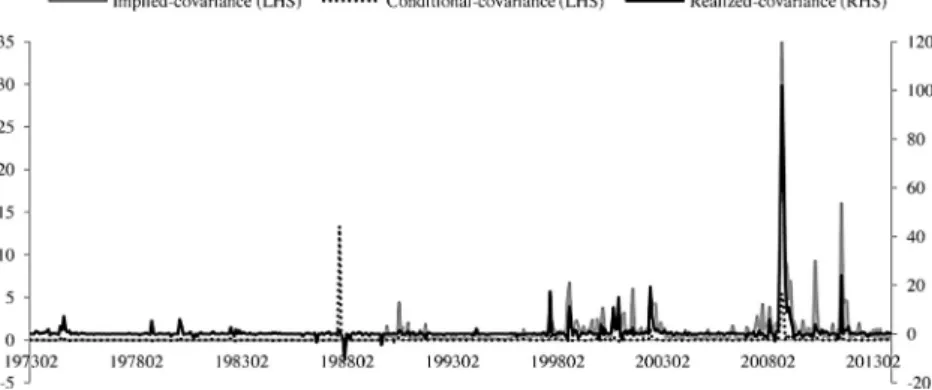
The covariance of return and volatility and the stock return volatility, defined in Eqs. (1) and (2), for k= realized, conditional and implied, are reported inFigs. 1 and 2, respectively. Realized-covariance shows more extreme values than the corresponding conditional and implied measures, and realized-covariance also includes many negative values. Values for realized and implied measures of covk
mare highest immediately after the globalfinancial crisis, with peak months being
October and November 2008. The implication is that, return for given volatility is highest during these months. Following the globalfinancial crisis, local peaks in realized and implied measures of covk
moccur in May 2010, when world stock markets fell
sharply during aflare up of the Eurozone crisis, and in August 2011, a month during which Standard and Poor downgraded U.S. sovereign debt and the U.S. and other global stock markets crashed. The peak value for conditional measure of the covariance of return and volatility, covconditional
m , is during October 1987, a month that includes‘Black Monday’, October 19,
1987, when the DJIA dropped by over 22%. 3.2. Structural VAR model
We utilize a structural vector autoregression (SVAR) model to examine the effects of oil price shocks identified and differentiated according to their supply and demand-side sources and their relation to the U.S. stock market return, volatility, and covariance, respectively. Oil price shocks can affect stock price return and volatility by effects on expected corporate cash flow and on the discount rate applied to future earnings (through expected inflation and expected real interest rate).
The structural vector autoregression model of orderjis in the following: B0Xt¼c0þ
Xj i¼1
BiXtiþ
e
t (3)whereXtis a 41 vector of endogenous variables,B0denotes a 44 contemporaneous coefficient matrix,c0represents a 41 vector of constant terms,Birefers to the 44 autoregressive coefficient matrices, and
e
tstands for a 41 vector ofstructural disturbances. The block of the endogenous variablesXt includes the percent change in world oil production
ð
D
prodtÞ, global real aggregate demand reað tÞ, and the real price of oilðrpotÞ.Kilian (2009)notes that this block captures thesupply and demand conditions in the world oil market and attributes thefluctuation of oil prices to oil supply-side shocks, shocks to the aggregate demand, and the oil-market specific demand shocks. The second block includes the U.S. stock market real return, volatility or covariance.
To construct the structural VAR representation (3), wefirst need to consistently estimate its reduced-form using the least-squares method. The reduced-form VAR model is obtained by multiplying both sides of Eq. (3) withB1
0 which is
[(Fig._1)TD$FIG]
Fig. 1.Monthly covariance of stock market return and volatility.
Note: The monthly covariance of stock market return and volatility is constructed from daily data on stock market return and daily volatility and defined in
Eq. (1). The measures of daily volatility are realized-volatility at high frequency (normalized squared return), conditional-volatility recovered from a
stochastic volatility model, and implied-volatility deduced from options prices. Realized-covariance and conditional-covariance are over 1973:01–2013:12
and implied-covariance is over 1990:01–2013:12.
postulated to have a recursive structure such that the reduced form errorsetare linear combinations of the structural errors
e
tin the following: et¼ eDtprod erea t erpot ecov t 0 B B @ 1 C C A¼ b11 0 0 0 b21 b22 0 0 b31 b32 b33 0 b41 b42 b43 b44 0 B B @ 1 C C Ae
Dprod te
rea te
rpo te
cov t 0 B B @ 1 C C A (4) wheree
Dprodt reflects oil supply shocks,
e
reat captures aggregate demand shocks,e
rpo
t denotes oil market-specific demand
shocks, and
e
covt is the return and volatility covariance shocks.
FollowingKilian (2009), we takej¼24, because the long lag of 24 allows for a potentially long delay in the shock effects of oil prices and for a sufficient number of lags to remove serial correlation.9The previous literature has shown that long lags are important in structural models of the world oil market to account for the low frequency co-movement between the real price of oil and global economic activity.Hamilton and Herrera (2004)argue that a lag length of 24 months is sufficient to capture the dynamics in the data in modeling business cycles in commodity markets. Ciner (2013) also emphasizes importance of the use of long lags in that oil price shocks that persist more (less) than a year have a positive (negative) impact on stock returns.
The exclusion restrictions onB01in the structural VAR model are based on the assumption inKilian and Park (2009). The supply of crude oil is inelastic in the short run, in the sense that the oil supply does not respond to contemporaneous changes in oil demand within a given month because of the high adjustment cost of oil production. Thefluctuation of real prices of oil does not lower global real economic activity within a given month because of slow global real reaction. In line with the standard approach of treating innovations to the price of oil as predetermined with respect to the economy (e.g.,Lee and Ni (2002)), we rule out instananeous responses from shocks to oil prices in the world oil market to the U.S. stock market. A recent study byKilian and Vega (2011)finds that there is no significant evidence of feedback within a given month from U.S. aggregates to the price of crude oil.
Notice that in Eq. (4)etN0;
S
in the reduced-form VAR model and the partial correlation coefficients quantify thecontemporaneous correlation between two components of the error terms,
r
ij¼ sij=ffiffiffiffiffiffiffiffiffiffi
d
iid
jjp
; where
s
ij denotes theelements of the precision matrix
S
1;and is given by:re a r po cov
D
prod 0:049 0:050 0:089 ð0:53Þ ð0:45Þ ð0:93Þ r ea 0:147 0:220 ð1:46Þ ð2:20Þ r p o 0:250 ð2:11Þ 2 6 6 6 6 6 6 6 6 4 3 7 7 7 7 7 7 7 7 5 : (5)The values in the parenthesis of the matrix in(5)are absolutet-statistic to the standard error generated by recursive-design wild bootstrap with 2000 replications proposed byGonçalves and Kilian (2004). The covariance refers to implied-covariance. When realized/conditional-covariance is used, we obtain similar results. This provides us with supporting evidence on the
[(Fig._2)TD$FIG]
Fig. 2.Monthly volatility of stock market return.
Note: The monthly variance of stock market return is constructed from daily data on stock market return and daily volatility and defined in Eq.(2).
The measures of daily volatility are realized-volatility at high frequency (normalized squared return), conditional-volatility recovered from a
stochastic volatility model, and implied-volatility deduced from options prices. Realized variance and conditional variance are over 1973:01–2013:12 and
implied-variance is over 1990:01–2013:12.
9
Sims (1998)andSims et al. (1990)argue that even a variable that displays no inertia does not necessarily show absence of long lags in regressions on other variables.
exclusion restrictions (shocks to oil prices predetermined to the economy), because the contemporaneous correlations between oil price shocks, and stock market return and volatility covariance are small and statistically insignificant within a given month.10As a consequence, the exclusion restrictions onB1
0 in the structural VAR model are appropriate. The stationarity of the variables in the model is investigated by conducting Augmented Dicky–Fuller (ADF), Phillips–Perron (PP), and Kwiatkowski–Phillips–Schmidt–Shin (KPSS) tests for each of the series, thefirst difference of the natural logarithm of oil production, aggregate demand, real oil price, and stock market return and volatility covariance. Table 1shows that we can reject the null hypothesis, based on the ADF, PP, and KPSS tests, that
D
prodt;reat;and covtcontaina unit root at the 1% significant level. We alsofind that the three tests suggest that real price of oilðrpotÞcontains a unit root.
The nonstationarity of real oil prices may lead to a loss of a symptotic efficiency as reflected in wider error bands in the estimation. However, taking thefirst difference may result in removal of the slow moving component in the series, and incorrectly differencing can cause the estimates to be inconsistent given the nature of standard unit root tests (e.g.,Kilian and Murphy (2014)). Since the estimated impulse response is robust, even if the stationary assumption is violated, we use the level of the real price of oil in common with prior oil literature (e.g.,Kilian and Park (2009)).
4. Empirical results
4.1. Impulse responses to oil market structural shocks
We report the impulse response functions (IRFs) of the covariance of stock return and volatility and of volatility over 24 months to one-standard deviation structural oil market shocks (global oil production, global real economic activity and real price of oil). One-standard error and two-standard error bands, indicated by dashed and dotted lines, respectively, are computed by conducting recursive-design wild bootrap with 2000 replications proposed byGonçalves and Kilian (2004). The analysis of the IRFs presents the short-run dynamic response of dependent variables (i.e., vertical axis labels) to the structural shocks.
4.1.1. Responses of covariance of return and volatility
The cumulative impulse responses to the structural oil market shocks for the covariance of stock return and realized-volatility (realized-covariance) are shown inFig. 3A, for the covariance of stock return and conditional-volatility (conditional-covariance) is shown in Fig. 3B, and for the covariance of stock return and implied-volatility (implied-covariance) is shown inFig. 3C. In eachfigure the responses arefirst to shocks to a reduction in global oil production, second to a positive innovation in global real economic activity, and third to a positive shock to the real price of oil.
A positive shock to global aggregate demand is associated with negative effects on the covariances of return and volatility in Figs. 3A–3C . The negative effect is statistically significant in the 4th month for realized-covariance, in the 1st, 4th, and 5th months for conditional-covariance, and in the 4–6th, 10th and 11th months for implied-covariance. Positive shocks to oil-market specific demand have a statistically significant negative effect on the return and volatility covariance relationships in Figs. 3A–3C over thefirst four tofive months of the shock, with the largest impact being achieved in the 3rd month.
InFigs. 3A and 3B, unanticipated disruptions of crude oil supply do not have a statistically significantly effect on realized or conditional-covariance. In contrast, inFig. 3C, an unanticipated reduction in crude oil production is associated with a statistically significant increase in implied-covariance of return and volatility, with the effect building up over several months, before starting to futher rise between the 13th and 24th months. Ourfindings suggest that the forward-looking Table 1
Results of stationarity test.
Variables ADF test PP test KPSS test
Without trend With trend Without trend With trend Without trend With trend
Dprod 10.994*** 11.004*** 25.182*** 25.161*** 0.041 0.030 rea 4.010*** 4.035*** 3.456*** 3.450*** 0.409*** 0.407*** rpo 1.621 1.686 2.068 2.129 1.250*** 1.209*** covrealized 7.144*** 7.334*** 9.546*** 9.623*** 0.407* 0.068 covimplied 5.777*** 6.620*** 9.594*** 10.238*** 1.681*** 0.081 covconditional 8.024*** 8.100*** 18.406*** 18.430*** 0.166 0.040
Notes: The null hypotheses for ADF and PP are: the series has a unit root I(1), whereas the null hypothesis of the KPSS test is: the series is stationary I(0). *, **,
and *** denote the significant level at 1%, 5%, and 10% level, respectively. The prod is thefirst difference of the natural logarithm of oil production, rea is real
aggregate demand, rpo is the natural logarithm of real price of oil, cov is the stock market return and volatility covariance, andDis thefirst difference
operator.
10
Swanson and Granger (1997)suggest using the value of partial correlation coefficients to determine the variable ordering and relevant t-statistics for identifying restriction on the VAR models.
implied-volatility may provide additional information compared to the current-looking conditional- and realized-measures as prior studies have concluded (e.g.,Andersen et al. (2005)).
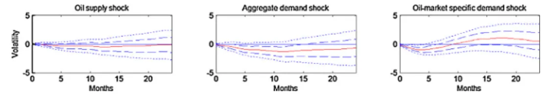
4.1.2. Responses of volatility
We now briefly examine the effect of oil supply and demand side shocks on U.S. stock market volatility. In the Eq. (3), stock market volatility is ordered last instead of covariance. Thus, the block of the endogenous variablesXtincludes the percent
change in world oil production
D
prodt
, global real aggregate demand reað tÞ, the real price of oil rpoð tÞ, and stock market
return volatility (volkm;k¼realized;conditional;implied). The cumulative impulse responses to the structural oil market
shocks for realized-volatility, conditional-volatility, and implied-volatility are shown in Figs. 4A–4C, respectively.11 A positive shock to global aggregate demand is associated with negative effects on volatility in Figs. 4A–4C. The negative effect is statistically significant between the 4th and 12th months for implied-variance. Positive shocks to oil-market specific demand have a statistically significant negative effect on each of the measures of volatility over thefirst three to four months
[(Fig._3A)TD$FIG]
Fig. 3A. Cumulative impulse responses of realized-covariance.
Note:Fig. 3Ashows cumulative responses of covariance using realized-volatility to structural oil shocks based on the structural VAR Eq. (3) in the text.
[(Fig._3B)TD$FIG]
Fig. 3B.Cumulative impulse responses of conditional-covariance.
Note:Fig. 3Bshows cumulative responses of covariance using conditional-volatility to structural oil shocks based on the structural VAR Eq. (3) in the text.
[(Fig._3C)TD$FIG]
Fig. 3C.Cumulative impulse responses of implied-covariance.
Note: Fig. 3C shows cumulative responses of covariance using implied-volatility to structural oil shocks based on the structural VAR Eq. (3) in the text.
[(Fig._4A)TD$FIG]
Fig. 4A. Cumulative impulse responses of realized-volatility.
Note: Fig. 4A shows cumulative responses of realized-volatility to structural oil shocks based on the structural VAR Eq. (3) in the text.
11
With regard to real stock returns, an unexpected expansion in the global real aggregate demand causes a significant increase in real stock return from
the 1st to the 10th month. Shocks to oil-market specific demand causes a persistent decrease in stock return after the 8th month. Unanticipated disruptions
of oil supply do not have a significant effect on the real stock return. These results are consistent with thefinding inKilian and Park (2009)who argue that
the impact of oil price shocks on U.S. real stock returns are predominantly by oil demand side shocks.
of the shock. This result is slightly different from thefinding byDegiannakis et al. (2014)using European stock market data that show oil-market specific demand has a negative effect on volatility that is only statistically significant at impact.
In Figs. 4A and 4B, unanticipated disruptions of crude oil supply do not have a statistically significantly effect on realized or conditional-volatility. This result is the same as thefinding byDegiannakis et al. (2014) that realized and conditional-volatility for European stock market data are not significantly impacted by oil supply surprises. InFig. 4C, an unanticipated reduction in crude oil production is associated with a statistically significant increase in implied-volatility over 5–9th and 18–24th months. This latter result contrasts with that byDegiannakis et al. (2014)(for implied-volatility for European stock market data) whofind that oil supply distruptions are associated with increases in implied-volatility for only thefirst two months, and these effects are not statistically significant.12
4.2. Variance decompositions and spillovers of return/volatility relationship
We now examine the forecast error variance decomposition (FEVD) showing the percent contribution of structural shocks in the crude oil market to the overall variation of the covariance of stock return and stock return volatility. The FEVDs quantify how important the three structural oil price shocks have been on average for the return and volatility covariance in the stock market. In addition, to provide greater understanding of interdependence of the oil market and the stock market, we follow Diebold and Yilmaz (2009, 2013) and report the spillover from the variance decomposition associated with the variables in the SVAR model in Eq. (3).
4.2.1. Variance decompositions
InTable 2, panels A1, B1, and C1 report FEVD results for realized, conditional, and implied-covariances, respectively. The values in parentheses inTable 2represent the absolutet-statistics when coefficients’standard errors were generated using a recursive-design wild bootstrap. Shocks to crude oil production explain a statistically significant 14.7% of the variation in the implied-covariance of return and volatility at the 60 month horizon. Shocks to crude oil supply do not explain a statistically significantly amount of variation in realized or conditional-covariance. In thefirst few months the effects of aggregate demand shocks on the covariances of return and volatlity are negligible and not statistically significant. Over time, the explanatory power of aggregate demand shocks on the covariances of return and volatility increase in size and statistical significance. At the 60 month horizon, aggregate demand shock explains 9.2% of realized-covariance, 7.9% of conditional-covariance, and 13.7% of implied-covariance of return and volatility.
Oil-market specific demand shocks explain a statistically significant 28.1% of variation in realized-covariance, a marginally statistically significant 10.2% of conditional-covariance at the 60 month horizon, and a statistically significant 33% of the variation in the implied-covariance of return and volatility. Overall, the largest percent contribution of structural shocks in the crude oil market to covariance of stock return and stock return volatility is when volatility is based on implied-volatility. Over a 60-month period shocks to oil supply disruptions, shocks to aggregate demand, and oil-market specific demand disturbances explain statistically significant 14.7%, 13.7%, and 33% of the variation in the implied-covariance of return and volatility, respectively, (in Panel C1 ofTable 2).
[(Fig._4B)TD$FIG]
Fig. 4B.Cumulative impulse responses of conditional-volatility.
Note: Fig. 4B shows cumulative responses of conditional-volatility to structural oil shocks based on the structural VAR Eq. (3) in the text.
[(Fig._4C)TD$FIG]
Fig. 4C.Cumulative impulse responses of implied-volatility.
Note: Fig. 4C shows cumulative responses of implied-volatility to structural oil shocks based on the structural VAR Eq. (3) in the text.
12
The data period forDegiannakis et al. (2014)also differs from that in this study. The data inDegiannakis et al. (2014)are for Eurostoxx 50 index from
January 1999-December 2010.
4.2.2. Spillover of oil market and the stock market
In Panel A2 (B2 and C2) ofTable 2, the off-diagonal elements give the 24-step ahead forecast error variance of a variable coming from shocks arising in the other variable using realized (conditional and implied) covariance. The value 1=4sum of off-diagonal elements provides us with the spillover index measuring the degree of connectedness for the oil market and the stock market. The spillover index 0.256 (0.207 and 0.359) for realized-covariance (conditional-covariance and implied-covariance) is highly statistically significant and reinforces thefinding that oil price shocks and the connection between stock market return and volatility are interrelated.
Table 2
Forecast error variance decomposition (FEVD) of stock return and volatility covariance.
Horizon Oil supply shock Aggregate demand shock Oil-market specific demand shock Other shocks
Panel A1. Realized-covariance
1 0.002 (0.37) 0.042 (1.21) 0.060 (1.44) 0.896 (13.37) 3 0.002 (0.34) 0.047 (1.29) 0.184 (2.43) 0.766 (9.14) 12 0.013 (0.77) 0.051 (1.50) 0.283 (3.43) 0.653 (8.01) 24 0.018 (0.90) 0.082 (2.10) 0.286 (3.85) 0.614 (8.07) 60 0.020 (0.95) 0.092 (2.35) 0.281 (4.03) 0.607 (8.27) Spillover index: 0.256 (6.38)
Panel A2. Spillover table when forecast horizon H = 24 for realized-covariance Contributions from
Contributions to (1) Oil supply shock (2) Aggregate demand shock (3) Oil-market specific demand shock (4) Other shocks
(1) 0.921 (31.32) 0.039 (2.09) 0.027 (1.57) 0.014 (1.08) (2) 0.021 (0.43) 0.845 (8.27) 0.030 (0.68) 0.105 (1.21) (3) 0.006 (0.19) 0.316 (2.49) 0.634 (4.93) 0.045 (0.76) (4) 0.018 (0.91) 0.082 (2.10) 0.286 (3.82) 0.614 (8.06) Spillover index: 0.256 (6.38) Panel B1. Conditional-covariance
Horizon Oil supply shock Aggregate demand shock Oil-market specific demand shock Other shocks
1 0.000 (0.08) 0.020 (0.54) 0.007 (0.27) 0.973 (17.12)
3 0.002 (0.21) 0.032 (0.77) 0.042 (0.76) 0.925 (11.06)
12 0.021 (0.70) 0.052 (1.21) 0.074 (1.08) 0.853 (8.13)
24 0.043 (1.02) 0.075 (1.64) 0.097 (1.38) 0.785 (7.02)
60 0.050 (1.19) 0.079 (1.73) 0.102 (1.46) 0.770 (6.79)
Panel B2. Spillover table when forecast horizon H = 24 for conditional-covariance Contributions from
Contributions to (1) Oil supply shock (2) Aggregate demand shock (3) Oil-market specific demand shock (4) Other shocks
(1) 0.901 (27.69) 0.040 (2.18) 0.027 (1.53) 0.032 (1.44) (2) 0.014 (0.30) 0.877 (8.57) 0.034 (0.61) 0.075 (0.89) (3) 0.006 (0.17) 0.382 (2.78) 0.610 (4.48) 0.002 (0.07) (4) 0.043 (1.03) 0.075 (1.64) 0.097 (1.38) 0.785 (7.05) Spillover index: 0.207 (4.73) Panel C1. Implied-covariance
Horizon Oil supply shock Aggregate demand shock Oil-market specific Demand shock Other shocks
1 0.005 (0.27) 0.072 (1.25) 0.058 (1.17) 0.866 (9.87)
3 0.045 (1.04) 0.046 (1.02) 0.249 (2.79) 0.661 (6.64)
12 0.079 (1.54) 0.073 (1.61) 0.395 (4.83) 0.454 (5.69)
24 0.144 (2.44) 0.094 (2.02) 0.361 (5.15) 0.401 (5.98)
60 0.147 (2.67) 0.137 (2.69) 0.330 (5.19) 0.386 (6.24)
Panel C2. Spillover table when forecast horizon H = 24 for implied covariance Contributions from
Contributions to (1) Oil supply shock (2) Aggregate demand shock (3) Oil-market specific demand shock (4) Other shocks
(1) 0.825 (17.47) 0.100 (2.89) 0.048 (1.77) 0.027 (1.13)
(2) 0.048 (0.55) 0.770 (5.84) 0.165 (1.49) 0.016 (0.31)
(3) 0.057 (0.79) 0.292 (2.32) 0.569 (4.34) 0.082 (1.03)
(4) 0.144 (2.44) 0.094 (1.99) 0.361 (5.24) 0.401 (5.95)
Spillover index: 0.359 (7.97)
Notes:Table 2shows percent contributions of demand and supply shocks in the crude oil market to the variability of stock return and volatility covariance. The forecast error variance decomposition is based on the structural VAR model described in the text. The values in parentheses represent the absolute
t-statistics when coefficients’standard errors were generated using a recursive-design wild bootstrap.
4.3. Variance decompositions of stock return volatility
Table 3reports the contributions of structural oil shocks to the variation of stock return volatility. InTable 3shocks to crude oil production and to aggregate demand do not explain a statistically significantly amount of variation in realized or conditional-volatility. Shocks to crude oil production explain a statistically significant 12.4% of the variation in the implied-volatility of return at the 60 month horizon. At the 60 month horizon, aggregate demand shocks explain a statistically significant 12.9% of implied-volatility.
Table 3
Forecast error variance decomposition (FEVD) of stock volatility.
Horizon Oil supply shock Aggregate demand shock Oil-market specific demand shock Other shocks
Panel A1. Realized-volatility
1 0.001 (0.14) 0.008 (0.30) 0.011 (0.55) 0.980 (24.15)
3 0.002 (0.26) 0.019 (0.57) 0.037 (1.02) 0.942 (16.62)
12 0.010 (0.50) 0.042 (1.01) 0.115 (2.04) 0.834 (11.95)
24 0.015 (0.59) 0.047 (1.20) 0.127 (2.18) 0.812 (11.54)
60 0.016 (0.63) 0.067 (1.34) 0.124 (2.22) 0.792 (10.49)
Panel A2. Spillover table when forecast horizonH= 24 for realized-volatility
Contributions from
Contributions to (1) Oil supply Shock (2) Aggregate demand shock (3) Oil-market specific demand shock (4) Other ocks
(1) 0.901 (29.25) 0.039 (2.20) 0.027 (1.57) 0.033 (1.87) (2) 0.013 (0.29) 0.898 (9.53) 0.034 (0.62) 0.054 (0.76) (3) 0.006 (0.17) 0.400 (2.94) 0.590 (4.45) 0.004 (0.11) (4) 0.015 (0.58) 0.047 (1.22) 0.127 (2.15) 0.812 (11.49) Spillover index: 0.200 (4.80) Panel B1. Conditional-volatility
Horizon Oil supply shock Aggregate demand shock Oil-market specific demand shock Other shocks
1 0.000 (0.00) 0.006 (0.21) 0.026 (0.92) 0.969 (20.14)
3 0.002 (0.26) 0.016 (0.46) 0.058 (1.30) 0.924 (14.08)
12 0.008 (0.40) 0.042 (0.90) 0.117 (2.00) 0.834 (11.25)
24 0.013 (0.45) 0.044 (1.05) 0.131 (2.12) 0.813 (11.01)
60 0.014 (0.49) 0.068 (1.30) 0.129 (2.16) 0.790 (10.16)
Panel B2. Spillover table when forecast horizonH= 24 for conditional-volatility
Contributions from
Contributions to (1) Oil supply shock (2) Aggregate demand shock (3) Oil-Market Specific demand shock (4) Other shocks
(1) 0.895 (28.38) 0.039 (2.22) 0.027 (1.56) 0.040 (1.97) (2) 0.013 (0.29) 0.912 (9.94) 0.033 (0.58) 0.042 (0.65) (3) 0.006 (0.20) 0.411 (3.03) 0.579 (4.40) 0.004 (0.13) (4) 0.013 (0.45) 0.044 (1.06) 0.131 (2.11) 0.813 (11.03) Spillover index: 0.200 (4.76) Panel C1. Implied-volatility
Horizon Oil supply shock Aggregate demand shock Oil-market specific demand Shock Other shocks
1 0.003 (0.18) 0.046 (1.08) 0.014 (0.50) 0.937 (16.53)
3 0.014 (0.55) 0.037 (0.99) 0.078 (1.25) 0.871 (11.53)
12 0.072 (1.51) 0.089 (1.75) 0.214 (2.96) 0.625 (7.67)
24 0.118 (2.11) 0.104 (2.23) 0.201 (3.28) 0.577 (7.92)
60 0.124 (2.31) 0.129 (2.34) 0.204 (3.46) 0.544 (7.71)
Panel C2. Spillover table when forecast horizonH= 24 for implied-volatility
Contributions from
Contributions to (1) Oil supply shock (2) Aggregate demand Sshock (3) Oil-Market specific demand shock (4) Other shocks
(1) 0.832 (17.69) 0.095 (2.82) 0.047 (1.77) 0.026 (1.09)
(2) 0.059 (0.66) 0.760 (5.87) 0.152 (1.36) 0.029 (0.51)
(3) 0.057 (0.77) 0.298 (2.27) 0.609 (4.59) 0.035 (0.56)
(4) 0.118 (2.13) 0.104 (2.32) 0.201 (3.28) 0.577 (7.93)
Spillover index: 0.305 (6.53)
Notes:Table 3shows percent contributions of demand and supply shocks in the crude oil market to the variability of stock volatility. The forecast error
variance decomposition is based on the structural VAR model described in the text. The values in parentheses represent the absolutet-statistics when
coefficients’standard errors were generated using a recursive-design wild bootstrap.
Oil-market specific demand shocks explain statistically significant fractions of the variation in all three measures of stock return volatility at the 12 month, 24 month, and 60 month horizons. At the 60 month horizon oil-market specific demand shocks forecast 12.4%, 12.9%, and 20.4% of variation in realized-volatility, conditional-volatility, implied-volatility of return, respectively. The largest percent contribution of structural shocks in the crude oil market to volatility of stock return is when volatility is based on implied-volatility. Over a 60-month period, the structural oil shocks forecast 45.7% of the variation in implied-volatility, in constrast to 20.8% of the variation in realized-volatility and 21% of the variation in conditional-volatility.
InTable 3, the spillover index for oil price shocks and the volatility of stock return is 0.200 (0.200 and 0.305) for realized (conditional and implied) volatility, and is highly statistically significant. Comparison of results inTables 2 and 3shows that for realized and implied-volatility, the spillover between oil price shocks and covariance of return and volatility is higher than the spillover between oil price shocks and volatility.
4.4. Rolling sample analysis
We now examine the effect of the structural oil market shocks on the return and volatility relationship overtime. In recent years, there have been dramatic pricefluctuations in the price for crude oil as well as majorfluctuation in the stock market. To investigate changes in the dynamics of the interaction of the global oil market and U.S. stock market, we estimate the structural VAR model with 180-month rolling samples starting in January 2005.13For each rolling SVAR estimation the spillover index is obtained.
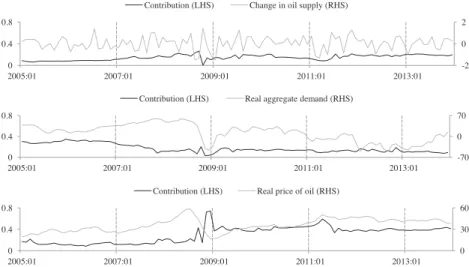
Fig. 5displays the evolution of the contribution of oil supply and demand side shocks to the forecast error variance of the implied-covariance of return and volatility after 24 months, along with the actual time series relative to its baseline forecast. InFig. 5, the top panel shows the contribution of global oil supply disturbances, the middle panel the contribution of global aggregate demand, and the bottom panel the contribution of oil-market specific demand.
Global oil production predicts 14.7% of the variation of implied-covariance of return and volatility overall (inTable 2), but the forecast amount was 8.4% over 2005–2006 before rising to an average of 21.3% from March to September in 2008, and averaging values 18.6% over 2011:07–2013:12. In juxtaposition the contribution of global aggregate demand to forecasting the implied-covariance of return and volatility is greater over 2005–2006 (about 30.0%), than subsequently. Over 2011:01–2013:12, global aggregate demand forecastes 11.5% of the implied-covariance of return and volatility. The decline in the relative contribution of oil production shocks, and the increase over time in the relative contribution of global aggregate demand shocks to forecasting the implied-covariance of stock return and volatility seems to occur gradually over 2007, and thus, predates the full onset of the globalfinancial crisis (on 15 September 2008 with Lehman Brothersfiling for bankruptcy).
Change in the ability of oil-market specific demand shocks to forecast the implied-covariance of stock return and volatility is different from that of the other two structural oil shocks. There is a sharp increase in fraction of volatility in
[(Fig._5)TD$FIG]
Fig. 5.Dynamic contributions to the variation of implied-covariance of stock market return and volatility, 2005:01–2013:12.
Note: Variance decomposition contributions to the variation of implied-covariance of stock market return and volatility after 24 months described in the text and estimated using 180-month rolling windows.
13
The time-varying relationship between the covariance of stock return and volatility and oil price movement could also be examined in terms of changes
in the correlations between these variables along the lines of the time-varying multivariate heteroskedastic framework inDegiannakis et al. (2013).
implied-covariance of stock return and volatility explained from 17.63% in August 2008 to 43.09% in September 2008. Following the globalfinancial crisis, oil-market specific demand shocks (oil price movement not explained by shocks to global oil production and global aggregate demand) forecast a much larger fraction of implied-covariance of stock return, and volatility than in the years immediately preceeding the globalfinancial crisis. Oil-market specific demand shocks forecast 14% of variation in implied-covariance of stock return and volatility before August/September 2008, and 41.6% after these dates.
5. Robustness check
We now perform some variations on our basic analysis of the effects of oil shocks on the covariance of stock return and volatility to check the robustness of results with respect to the lag length of the structural VAR model, the forecast horizon, and results for a normalization of the covariance of stock returns with volatility. When the forecast error variance decomposition is based on the structural VAR model by taking shorter 12 lags and shorter 12 forecast horizon for the spillover table, results are similar to those already obtained inTable 2. In particular, the largest percent contribution of structural shocks in the crude oil market to covariance of stock return and stock return volatility is when covariance is based on implied-volatility. Over a 60-month period shocks to oil supply disruptions, shocks to aggregate demand, and oil-market specific demand disturbances explain statistically significant 7.7%, 15.0%, and 30.6% of the variation in the implied-covariance of return and volatility, respectively.14Outcomes slightly smaller than those noted for the model with longer lag lengths inTable 2.
Given the large values occasionally assumed by inFig. 1, we examine the response of the covariance of return and volatility normalized by volatility to structural oil shocks to determine if similar results hold for a smoother measure of covariance. Normalized covariance is defined as:
l
km¼covk m rdt;k
s
dt
volkm k
s
dt;k¼realized;conditional;implied; (6)
where covk m rdt;k
s
dt
and volkm k
s
dt
are given in Eqs.(1)and(2).
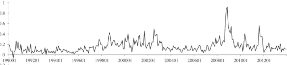
The ratio of implied-covariance of return and volatility to implied-volatility is shown inFig. 6. The range of values for
l
kminFig. 6is much narrower than that for either covariance of return and volatility inFig. 1. InFig. 6, the peak value for
l
kmis 0.885 in October 2008 and the only negative values ofl
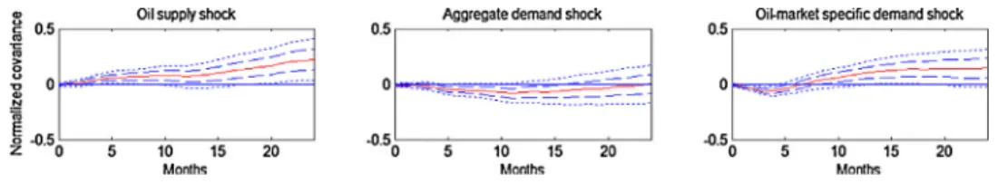
kmoccur in 1990:05 (0.068) and 1993:03 (0.007).The cumulative impulse responses to the structural oil shocks for the normalized covariance of stock return and implied-volatility are shown inFig. 7. A positive shock to global aggregate demand is associated with negative effects on the normalized covariance of return and volatility that are marginally significant over 5–10 months. Positive shocks to oil-market specific demand have a statistically significant negative effect on normalized covariance inFig. 7over thefirst four months of the shock. An unanticipated reduction in crude oil production is associated with an increase in normalized covariance, that is statistically significant over a number of months. Thus, impulse response result to structural oil price shocks is similar for normalized covariance of stock return and volatility and for covariance of stock return and volatility. 6. Conclusions
The study examines the effects of global oil price shocks on the stock market return and volatility contemporaneous relation using a structural VAR model. We construct from daily data measures of return and volatility the covariance of
[(Fig._6)TD$FIG]
Fig. 6.Normalized covariance of return and volatility.
Note:Fig. 6shows normalized implied-covariance of return and volatility, covk
m rdt;ksdt
,volk
m ksdr
defined in Eq. (6) over 1990:01–2013:12. The
monthly implied normalized covariance is constructed from monthly data on the implied-covariance of stock return and volatility and on implied-volatility, derived from daily data on stock market return and daily volatility. The measure of daily volatility is implied-volatility deduced from options prices.
14 Results are available upon request.
return and volatility at monthly frequency. The measures of daily volatility are realized-volatility at high frequency (normalized squared return), conditional-volatility recovered from a stochastic volatility model, and implied-volatility deduced from options prices. It is found that oil price shocks contain information for forecasting the contemporaneous relationship between stock return and stock volatility.
Positive shock to global aggregate demand is associated with negative effects on the covariances of return and volatility with the statistical significance of the effect extending for a longer period for implied-covariance. Positive shocks to oil-market specific demand have a statistically significant negative effect on the return and volatility covariance relationships for several months. An unanticipated reduction in crude oil production is associated with a statistically significant increase implied-covariance of return and volatility that extends for 24 months. The spillover index between the structural oil price shocks and covariance of stock return and volatility is highly statistically significant and is 35.9% for the covariance of return and implied-volatility.
The dynamic contributions of oil supply and demand side shocks to the covariance of stock return and volatility are calculated from a rolling SVAR model. Global oil production predicts 8.4% of the variance of implied-covariance of return and volatility over 2005–2006, before rising to an average of 21.3% from March to September in 2008 and averaging values 18.6% over 2011:07–2013:12. This contrasts with the contribution of global aggregate demand to forecasting the implied-covariance of return and volatility which is greater over 2005–2006 (about 30.0%), than subsequently (11.5% over 2011:01–2013:12). These changes occur gradually over 2007 and predate the full onset of the global financial crisis. Oil-market specific demand shocks forecast 14% of variation in implied-covariance of stock return and volatility before August/September 2008, and 41.6% after these dates.
There is a sharp increase in fraction of volatility in implied-covariance of stock return and volatility explained by oil-market specific demand shocks from 17.63% in August 2008 to 43.09% in September 2008. Following the globalfinancial crisis, oil-market specific demand shocks forecast a much larger fraction of implied-covariance of stock return and volatility than in the years immediately preceeding the globalfinancial crisis. These results might aid investors, researchers, or regulators interested in the determinants of the joint behavior, and risk-return trade-off of stock return and volatility. References
Abhyankar, A., Xu, B., Wang, J., 2013. Oil price shocks and the stock market: evidence from Japan. Energy J. 34, 199–222.
Andersen, T., Bollerslev, T., 1998. Answering the skeptics: yes standard volatility models do provide accurate forecasts. Int. Econ. Rev. 39, 885–905.
Andersen, T.G., Bollerslev, T., Meddahi, N., 2005. Correcting the errors: volatility forecast evaluation using high frequency data and realized volatilities. Econometrica 73, 279–296.
Apergis, N., Miller, S.M., 2009. Do structural oil-market shocks affect stock prices? Energy Econ. 31, 569–575.
Arouri, M.E.H., Rault, C., 2011. On the influence of oil prices on stock markets: evidence from panel analysis in GCC countries. Int. J. Financ. Econ. 3, 242–253.
Arouri, M.E.H., Jouini, J., Nguyen, D.K., 2012. On the impacts of oil pricefluctuations on European equity markets: volatility spillover and hedging effectiveness. Energy Econ. 34, 611–617.
R.B. Barsky, L. Kilian, Do we really know that oil caused the great stagflation? A monetary alternative, In NBER Macroeconomics Annual 2001, 2002, 16,
137–198.
Baum, C.F., Caglayan, M., Talavera, O., 2008. Uncertainty determinants offirm investment. Econ. Lett. 98, 282–287.
Blair, B.J., Poon, S.-H., Taylor, S.J., 2001. Forecasting S&P100 volatility: the incremental information content of implied volatilities and high-frequency index returns. J. Econometrics 105, 5–26.
Bollerslev, T., Zhou, H., 2006. Volatility puzzles: a simple framework for gauging return-volatility regressions. J. Econometrics 131, 123–150.
Chen, S.S., 2010. Do higher oil prices push the stock market into bear territory? Energy Econ. 32 (2), 490–495.
Ciner, C., 2013. Oil and stock returns: frequency domain evidence. J. Int. Financ. Markets Inst. Money 23, 1–11.
Connolly, R., Stivers, C., Sun, L., 2005. Stock market uncertainty and the stock-bond return relation. J. Financ. Quant. Anal. 40, 161–194.
Degiannakis, S., Filis, G., Floros, C., 2013. Oil and stock returns: evidence from European industrial sector indices in a time-varying environment. J. Int. Financ. Markets Inst. Money 26, 175–191.
Degiannakis, S., Filis, G., Kizys, R., 2014. The effects of oil price shocks on stock market volatility: evidence from European data. Energy J. 35, 35–56.
Ebens, H., 1999. Realized Stock Volatility. Johns Hopkins University, Department of Economics Working Paper 420.
Engle, R.F., 2002. New frontiers for ARCH models. J. Appl. Econometrics 17, 425–446.
Filis, G., Degiannakis, S., Floros, C., 2011. Dynamic correlation between stock market and oil prices: the case of oil-importing and oil-exporting countries. Int. Rev. Financ. Anal. 20, 152–164.
Fleming, J., Ostdiek, B., Whaley, R.E., 1995. Predicting stock market volatility: a new measure. J. Futures Markets 15, 265–302.
French, K.R., Schwert, G.W., Stambaugh, R.F., 1987. Expected stock returns and volatility. J. Financ. Econ. 19, 3–30.
Ghysels, E., Santa-Clara, P., Valkanov, R., 2005. There is risk-return trade-off after all. J. Financ. Econ. 76, 509–548.
Glosten, L.R., Jagannathan, R., Runkle, D.E., 1993. On the relation between the expected value and the volatility of nominal excess return on stocks. J. Financ. 48, 1779–1801.
[(Fig._7)TD$FIG]
Fig. 7.Normalized covariance of return and volatility.
Note:Fig. 7shows cumulative responses of normalized covariance of return and implied-volatility to structural oil shocks based on the structural VAR in the
text.
Gonçalves, S., kilian, L., 2004. Bootstrapping autoregressions with conditional heteroskedasticity of unknown form. J. Econometrics 123, 89–120.
Hamilton, J.D., 2009. Causes and consequences of the oil shock of 2007–08. Brookings Papers on Economics Activity. Spring, pp. 215–261.
Hamilton, J.D., Herrera, M., 2004. Oil shocks and aggregate macroeconomic behavior: the role of monetary policy: comment. J. Money Credit Banking 36, 265–286.
Hibbert, A.M., Daigler, R.T., Dupoyet, B., 2008. A behavioral explanation for the negative asymmetric return–volatility relation. J. Banking Financ. 32, 2254–2266.
Jimenez-Rodriguez, R., Sanchez, M., 2005. Oil price shocks and real GDP growth, empirical evidence for some OECD countries. Appl. Econ. 37, 201–228.
Jones, C.M., Kaul, G., 1996. Oil and the stock markets. J. Financ. 51, 463–491.
Kanas, 2012. Modelling the risk-return relation for the S&P 100: the role of VIX. Econ. Model. 29, 795–809.
Kilian, L.C., 2009. Not all oil price shocks are alike: disentangling demand and supply shocks in the crude oil market. Am. Econ. Rev. 99, 1053–1069.
Kilian, L., Park, C., 2009. The impact of oil price shocks on the U. S. stock market. Int. Econ. Rev. 50, 1267–1287.
Kilian, L., Murphy, D.P., 2014. The role of inventories and speculative trading in the global market for crude oil. J. Appl. Econ. 29 (3), 454–478.
Kilian, L., Vega, C., 2011. Do energy prices respond to U. S. macroeconomic news? A test of the hypothesis of predetermined energy prices. Rev. Econ. Stat. 93, 660–671.
Lee, C.F., Chen, G., Rui, O., 2001. Stock returns and volatility on China’s stock markets. J. Financ. Res. 26, 523–543.
Lee, K., Ni, S., 2002. On the dynamic effects of oil price shocks: a study using industry level data. J. Monetary Econ. 49, 823–852.
Li, Q., Yang, J., Hsiao, C., Chang, Y.-J., 2005. The relationship between stock returns and volatility in international stock markets. J. Empirical Financ. 12, 650–665.
Malik, F., Ewing, B.T., 2009. Volatility transmission between oil prices and equity sector returns. Int. Rev. Financ. Anal. 18, 95–100.
Merton, R.C., 1980. On estimating the expected return on the market: an exploratory investigation. J. Financ. Econ. 8, 323–361.
Miller, J.I., Ratti, R.A., 2009. Crude oil and stock markets: stability, instability, and bubbles. Energy Econ. 31 (4), 559–568.
Nandha, M., Faff, R., 2008.‘Does oil move equity prices? A global view’. Energy Econ. 30, 986–997.
Pagan, A., 1984. Econometric issues in the analysis of regressions with generated regressors. Int. Econ. Rev. 25, 221–247.
Papapetrou, E., 2001. Oil price shocks, stock market, economic activity and employment in Greece. Energy Econ. 23, 511–532.
Sadorsky, P., 1999. Oil price shocks and stock market activity. Energy Econ. 21, 449–469.
Sims, C.A., 1998. Econometric implications of the government budget constraint. J. Econometrics 83, 9–19.
Sims, C.A., Stock, J.H., Watson, M.W., 1990. Inference in linear time-series models with some unit roots. Econometrica 58, 113–144.
Swanson, N.R., Granger, C.W.J., 1997. Impulse response functions based on a causal approach to residual orthogonalization in vector autoregressions. J. Am. Stat. Assoc. 92, 357–367.
Theodossiou, P., Lee, U., 1995. Relationship between volatility and expected returns across international stock markets. J. Bus. Financ. Accoun. 22, 289–300.
Vo, M., 2011. Oil and stock market volatility: a multivariate stochastic volatility perspective. Energy Econ. 33, 956–965. 54 W. Kang et al. / Int. Fin. Markets, Inst. and Money 34 (2015) 41–54