Page 1 of 1
FedUni ResearchOnline
https://researchonline.federation.edu.au
Copyright NoticeThis is the peer-reviewed version of the following article:
Pang, M., Ting, K., Zhao, P., Zhou, Z. (2018) Improving deep forest by confidence
screening. 2018 IEEE International Conference on Data Mining; Singapore, Singapore; 17th-20th November 2018 p. 1194-1199.
Which has been published in final form at: https://doi.org/10.1109/ICDM.2018.00158
Copyright © 2018 IEEE. Personal use of this material is permitted. Permission from IEEE must be obtained for all other uses, in any current or future media, including reprinting/republishing this material for advertising or promotional purposes, creating new collective works, for resale or redistribution to servers or lists, or reuse of any copyrighted component of this work in other works.
Improving Deep Forest by Confidence Screening
Ming Pang
1,2, Kai-Ming Ting
3, Peng Zhao
1,2, Zhi-Hua Zhou
1,21National Key Laboratory for Novel Software Technology, Nanjing University, Nanjing 210023, China
2Collaborative Innovation Center of Novel Software Technology and Industrialization, Nanjing 210023, China
3School of Engineering and Information Technology, Federation University, Australia
Email:1,2{pangm, zhaop, zhouzh}@lamda.nju.edu.cn 3[email protected]
Abstract—Most studies about deep learning are based on
neural network models, where many layers of parameterized nonlinear differentiable modules are trained by backpropagation. Recently, it has been shown that deep learning can also be realized by non-differentiable modules without backpropagation training called deep forest. The developed representation learning process is based on a cascade of cascades of decision tree forests, where the high memory requirement and the high time cost inhibit the training of large models. In this paper, we propose a simple yet effective approach to improve the efficiency of deep forest. The key idea is to pass the instances with high confidence directly to the final stage rather than passing through all the levels. We also provide a theoretical analysis suggesting a means to vary the model complexity from low to high as the level increases in the cascade, which further reduces the memory requirement and time cost. Our experiments show that the proposed approach achieves highly competitive predictive performance with significantly reduced time cost and memory requirement by up to one order of magnitude.
I. INTRODUCTION
Deep learning has achieved great success in various applica-tions, particularly with visual and speech information [1], [2]. Most studies about deep learning are based on neural network models, or more accurately, many layers of parameterized non-linear differentiable modules that can be trained by backpropa-gation. By recognizing that the keys of deep learning may lie in the layer-by-layer processing, in-model feature transformation and sufficient model complexity, Zhou and Feng [3] proposed a deep learning method named gcForest, which is realized by non-differentiable modules without backpropagation training. Essentially, gcForest is a novel decision tree ensemble method with predictive accuracy highly competitive to deep neural networks in a broad range of tasks. Besides, gcForest is much easier to train because it has fewer hyper-parameters. It has been shown that gcForest can achieve high predictive accuracy on datasets across different domains by using almost the same settings of hyper-parameters. Another advantage is that the model complexity of gcForest can be determined automatically for different training datasets, enabling gcForest to perform well even on small-scale datasets. In contrast, deep neural networks usually require a huge amount of training data which prevent them from being applied to small-scale datasets. A deep forest ensemble with a cascade structure enables gc-Forest to do representation learning. In this cascade structure, each level consists of an ensemble of decision tree forests [4], [5], i.e., an ensemble of ensembles [6]. Each level receives a new set of features as input which is the output of its preceding
level. For textual or structural data, gcForest further enhances its representational learning ability by a technique called multi-grained scanning.
Although the results in [7] suggest that larger models might tend to offer better accuracy, Zhou and Feng [3] have not tried larger models with more grains and larger number of forests and trees (in each forest) which is limited by the high memory requirement and time cost.
We identify that the main cause of this limitation owes much to two aspects. Firstly, gcForest passes all instances through all levels of the cascade, leading to a linear increase of time complexity w.r.t. the number of levels. Secondly, multi-grained scanning usually converts one (original) instance into hundreds or even thousands of new instances which significantly in-creases the number of training instances and also produces a high-dimensional input for the following cascade procedure.
To address these issues, we introduce aconfidence screening
mechanism in the general framework of deep forest, with the aim to reduce memory requirement and time cost. Specifically, the confidence screening categorizes instances at every level of the cascade into two subsets: one is easy to predict; and the other is hard. If an instance is easy to predict, its final prediction is produced at the current level; only if an instance is hard to predict, it needs to go through the next level (and potentially all levels in the cascade).
In addition, we provide a theoretical analysis which suggests a means to vary the model complexity from low to high as the level increases in the cascade. This design further reduces the memory requirement and time cost at the first few levels. Furthermore, we adopt a subsampling regime to significantly reduce the number of instances generated in the multi-grained scanning process.
In a nutshell, we propose an improved deep forest called gcForestcswhich is based on the confidence screening mecha-nism, coupled with a method to vary model complexity and the subsampling multi-grained scanning. Our experiments show that gcForestcs achieves predictive accuracy comparable to or better than gcForest. This is achieved with up to an order of magnitude lower memory requirement and faster runtime.
The rest of this paper is organized as follows. Section II pro-poses our method gcForestcs. Section III gives an analysis for the confidence screening mechanism. Section IV provides the discussion. Section V reports the empirical results. Section VI studies the influence of confidence screening. Section VII concludes this paper.
In pu t Fe at ur e Ve ct or Forest Forest Forest Forest Forest Forest Forest Forest Forest Forest Forest Forest
Level 1 Level 2 Level T
Ave. Max Fi na lPr ed ic tio n concatenate Y N N Y N Y Gate Gate Gate
(a) Cascade forest with confidence screening
Ra w In pu t F ea tu re s 400 -di m 100 -di m Sl id in g Forest A Forest B 30 3-di m 3-di m Concatenate 90 -dim 90 -dim Sl id in g Sliding 20×20 input 10-dim 10 10 10 3-di m 3-di m Concatenate 30 -dim 30 -dim Forest A Forest B
For sequence data
For image-style data
100 -di m 301 instances 100 -di m 30 instances 10 10 su bsa m pl in g su bsa m pl in g
(b) Feature re-representation using sliding window scanning withsubsampling
Fig. 1: gcForestcs: illustration of the cascade forest structure with confidence screeningand feature re-representation using sliding window
scanning withsubsampling regime. (a) Suppose there are two random forests (black) and two completely-random forests (blue) at each level
of the cascade. For a three-class problem, each forest outputs a three-dimensional class vector, which is concatenated for re-representation
of the original input. Instances with high prediction confidence (Y) at leveliare predicted directly—they do not go through all the levels.
Only instances with low prediction confidence (N) traverse to the next level. (b) Suppose there are three classes. Raw features are 400-dim,
sliding window is 100-dim and subsampling size is 30 for the sequence data; raw features are 20×20-dim, sliding window is 10×10-dim
and subsampling size is 10 for the image-style data.
II. THEPROPOSEDAPPROACH GCFORESTCS
The new deep forest approach gcForestcs has the key confidence screeningmechanism coupled with variable model complexity and subsampling multi-grained scanning to reduce the memory requirement and time cost of deep forest.
Rather than requiring all instances to go through all levels of cascade, we reduce the computation by requiring selective instances to go through the next level. The selection criterion
is based on the prediction confidencewhich is the maximum
value of the estimated class vector of one instance. For exam-ple, in a 3-class classification problem, as shown in Figure 2,
the estimated class vector of an instance is[0.7,0.2,0.1], then
its prediction confidence is 0.7.
The basic idea is that an instance is pushed to the next level only if it is determined to require a higher level of learning; otherwise, it is predicted using the model at the current level. Based on this idea, we propose the deep forest structure with gates for confidence screening as shown in Figure 1(a).
A deep forest model with confidence screening can be for-malized as follows. Consider the supervised learning problem
of learning a mapping from the feature space X to the label
space Y, where Y = {1,2, . . . , C}. Let Z = [0,1]C and
training setS= ((x1, y1), . . . ,(xm, ym))be drawn i.i.d. from
Forest … … 0.7 0.2 0.1 [ [ 0.8 0.0 0.2 [ [ 0.6 0.4 0.0 [ [ Ave. 0.7 0.2 0.1
[
[
𝑥 VectorClassFig. 2: Illustration of class vector generation from [3]. Each compo-nent of the final class vector is an average of the outputs of individual trees. Different shapes in leaf nodes denote different classes.
distributionD. A deep forest model with confidence screening
can be defined by a triplet(h,f,κ)where
• h= (h1, . . . , hT), wherehtis the ensemble of forests at
level t, andht is a member of hypothesis classHt.
• f = (f1, . . . , fT), where ft is the cascade of ensembles
of forests up to levelt.
• κ = (κ1, . . . , κT), where κt is a screener function:
κt(x) = 1if xis predicted byft,κt(x) = 0 otherwise.
At levelt∈ {1, . . . , T},ft: X → Z is defined as follows:
ft(x) = { h1(x) t= 1, ht ( [x, ft−1(x)] ) t >1. (1)
At every level t, ht(·) and ft(·) output a class vector
[pt1, . . . , ptC], where pi is the prediction confidence of class
i. The input ofht is[x, ft−1(x)]except at levelt= 1, where
its input isx.
Screener κt(·) at level t is defined based on prediction
confidence and confidence threshold ηt.
κt(x) =
{
1 maxc∈{1,...,C}[ft(x)]c > ηt,
0 otherwise. (2)
Let κ−t1(1) denote the set of instances such that κt(x) = 1,
which is the set of instances with high confidence at levelt.
κ−t1(0)is similarly defined for those with low confidence.
At level t, if the prediction confidence of one instance is
larger than threshold ηt, then its final prediction is produced
at the current level; otherwise it needs to go through the next level (and potentially all levels in the cascade).
Each triplet (h,f,κ) defines a deep forest model with
confidence screeningg:X → Y as follows:
g(x) = arg max c∈{1,...,C}
[
ft′(x)]c, (3)
wheret′= argt∈{1,...,T}κt(x) = 1.
The key issue here is how to set the confidence threshold at each level. In principle, one can define an optimization
Algorithm 1 gcForestcs
Input:Training setS, validation setSv, learning algorithmA
and the maximal number of cascade levels T.
Output: The gcForestcs model g.
Initialize: S1=S,ℓ0= 1andt= 1
Process:
1: whilet≤T do 2: ht=A(St).
3: Getftaccording to Eq. (1).
4: Getκt according to Eq. (2).
5: Getgtaccording to Eq. (3).
6: Compute the validation errorℓt=LSv(gt)
7: ifℓt> ℓt−1 then 8: return g. 9: end if 10: g=gt. 11: St+1 =St\κ−t1(1). 12: t=t+ 1. 13: end while 14: return g.
framework in which the confidence threshold at each level is set to trade off between minimizing the expected number of instances to be passed to the next level and maximizing the expected number of instances that can be corrected at the next level (which are misclassified at the current level.) Unfortunately, finding this optimum is a difficult problem.
Instead, we use a simple rule to produce an effective cascade forest which is highly efficient. The prediction confidence
threshold ηt at level t is determined automatically based on
the cross-validated error rate ϵt of all the training instances.
Let hyper-parametera <1be a fraction ofϵt. All the training
instances are sorted in descending order of their prediction
confidences, whereci is the prediction confidence ofxi.ηtis
set according to the following formulation:
ηt= min{ck|L(x1, . . . ,xk)< aϵt, k∈[1, m]}, (4)
where L(x1, . . . ,xk) = 1k
∑k
i=11[gt(xi) ̸= yi] is the error
rate of thekinstances with the largest prediction confidences.
Note that a is the only additional hyper-parameter for
confi-dence screening, compared with gcForest.
Variable model complexity. Because the remaining stances become increasingly hard-to-predict as the level in-creases, gcForestcs uses increasingly complex forests at high levels, i.e., gcForestcs increases the number of trees in each forest linearly as the number of training instances decreases.
The above strategy follows the result of the theoretical analysis in Section III. It suggests that varying the model complexity from low to high as the level increases in the cascade can lead to better generalization performance. This design further reduces memory requirement and time cost; and the model complexity only increases as the level increases when it is most needed to produce an accurate model for hard-to-predict instances. SN T S2Y SN2 S S1Y S1N S3Y … level 1 level 2 level 3 level T … h1 h2 h3 hT
Fig. 3: The structure of the cascade forest with confidence screening.
There is a total ofTlevels, where the instances are split into two parts
at each level: the left part contains instances with high confidence, and the right part contains those with low confidence and thus needs to be further processed at higher levels.
Subsampling multi-grained scanning.Multi-grained scan-ning in gcForest [3] increases the memory consumption and runtime heavily. To address this issue, as suggested in [3],
we use subsampling in multi-grained scanning. Specifically,
we randomly sample from the set of the converted instances produced in multi-grained scanning. As Figure 1(b) illustrates, subsampling not only reduces the number of converted in-stances, but also reduces the number of dimensions of the transformed features by an order of magnitude from 903 to 90 dimensions. At each level, subsampling multi-grained scanning generates new transformed features, and the features from the recent three levels are concatenated to classify the remaining instances which are fewer and “harder”.
Algorithm 1 summarizes the proposed gcForestcs.1
III. ANALYSIS
In this section, we provide an analysis for both the confi-dence screening and variable model complexity. In particular, we are interested in the effect of splitting all instances into two parts according to the prediction confidences, and thus, we ignore the effect of concatenation of previous label predictions in the analysis.
LetS ={(xi, yi)}mi=1 be the training set of sizemdrawn
according to the underlying distribution D, where xi ∈ Rd
andyi ∈ Y = {1,2, . . . C} is the associated class label. Let
the loss function beℓ:Y × Y →R+. For a given hypothesis
h, its riskR(h)and empirical risk RˆS(h)are:
R(h) =E(x,y)∼D[ℓ(h(x), y)], RˆS(h) = 1 m m ∑ i=1 ℓ(h(xi), yi).
An illustration of the cascade structure is given in Figure 3.
Suppose the cascade has T levels, and hash= (h1, . . . , hT)
with the classifier at level t ht: X →[−1,+1]; andht is a
member of the hypothesis set Ht. Note that we consider the
two-class problem only here for ease of analysis. Furthermore,
we denote Ht = {x → κt(x)ht(x) : κt ∈ Kt, ht ∈ Ht}
as the family of the products of the screener function and 1Note that subsampling multi-grained scanning can be used to provide a
the classifier at level t. Then we have the following results regarding the generalization bound of the learned model.
Theorem 1. Assume that the function in Ht takes values in
[−1,+1] for allt∈ {1, . . . , T}, and the training sampleS is
of size m drawn i.i.d. from underlying distribution D. Then,
for any δ > 0, with probability at least 1−δ, the following
holds for all hwithT levels cascade forest:
R(h)≤RˆS(h) + T ∑ t=1 min ( 4 ˆRS(Ht), mt m ) + ˜O ( T √ logT m ) ,
whereRˆSis the empirical Rademacher complexity, andmt=
|StY|is the number of screened instances at level t.
Proof. First, we introduce the convex ensembles with multiple
hypothesis setgα. For any α∈∆T, denotegα as follows,
gα(x) =
T
∑
t=1
αtκt(x)ht(x),
where ∆T is the simplex in RT. Fix ρ > 0, since gα is a
convex combination of the mappings x → κt(x)ht(x), and
note that h(x) = ∑Tt=1κt(x)ht(x), using Theorem 1 in [8],
we can obtain R(h)≤ inf α∈∆T [ ˆ RS,ρ(gα) + 4 ρ T ∑ t=1 αtRˆS(Ht) ] +C(m, p) + √ log(4/δ) 2m , (5) where C(m, ρ) = 2ρ √ logT m + √ logT ρ2m log ( ρ2m logT ) , and ˆ RS,ρ(gα) = m1 ∑T t=1 ∑ κ(xi,k)=1I[yiαtht(xi)< ρ].I[e(·)]is
the indicator function taking 1 ife(·)is true; and 0 otherwise.
The second step is to provide the upper bound for the first term in r.h.s. of Eq. (5). Following the analysis in [9],
inf α∈∆T [ ˆ RS,ρ(gα) + 4 ρ T ∑ t=1 αtRˆS(Ht) ] ≤Rˆ S(h) + T ∑ t=1 min ( 4 ˆRS(Ht), mt m ) + min I⊆T, |I|≥|T |−1/ρ ∑ t∈I (m t m −4 ˆRS(Ht) ) (6)
Hence, we complete the proof by combining (5) and (6),
R(h)≤RˆS(h) + T ∑ t=1 min ( 4 ˆRS(Ht), mt m ) +C(m, ρ) + min I⊆T, |I|≥|T |−1/ρ ∑ k∈I (m t m −4 ˆRS(Ht) ) + √ log(4/δ) 2m , where C(m, ρ) = 2ρ √ logT m + √ logT ρ2m log ( ρ2m logT ) ; and T =
{k:mt/m >4 ˆRS(Ht)}, the set of levelt whose screening
ratio is greater than 4 ˆRS(Ht).
To simplify the presentation, we ignore the non-leading
terms and only keep the terms regarding cascade level T,
instance number m and Rademacher complexity terms, and
obtain the simpler form as specified in Theorem 1.
Remark. The generalization error bound in Theorem 1 sheds light on the cascade structure design. Note that the second term
is the minimization of screening ratiomt/mand complexity
term4 ˆRS(Ht). Because most of the instances will be screened
in the first few levels, the screening ratio is large. Hence, one should reduce the corresponding complexity term in these few levels in order to make the generalization error bound tighter. This is the theoretical basis in which we vary the model complexity at a level in the cascade from low to high (by
increasing the ensemble size) as the levelt increases.
IV. DISCUSSION
The high memory requirement and time cost of gcForest can be tackled by exploiting distributed implementation [10] or hardware facilitation. We believe, however, there is demand to tackle them via algorithmic improvement.
The cascade procedure with confidence screening has some connection with two lines of research. First, confidence screen-ing is related to boosted cascade [11] which aims to reject many negative instances and has achieved success in visual object detection problems. Although the cascade structure appears to be similar on the surface, the boosted cascade procedure is not suitable for classification tasks because the nature of the object detection tasks is different.
Second, there are some studies which add the output of one classifier as an additional input for another classifier in a series of multiple classifiers to improve the accuracy of a single classifier [12], [13]. Like gcForest, these methods pass all the instances through all the classifiers which is inefficient. The subsampling strategy is related to sampling strategies for bag-of-features image classification [14], [15]. By treating an image as a collection of independent patches, random sampling gives equal or better representative selection than the sophisticated multiscale interest operators. In this paper, we use a simple random sampling strategy and show that it works in the context of deep forest. It is interesting to explore other sampling strategies [16], [17].
In addition, using more features for the low-confidence instances is related to the time-efficient feature extraction approach [18]. For test instances, this approach only extracts cheap and sufficient features, and when the classification confidence is high enough, the test instance will be classified. There are two main differences between this work and our approach. First, their goal is to reduce test time cost, while our goal is to reduce both train and test time cost of gcForest. Second, features are given with known feature extraction time costs in their setting, while the transformed features in deep forest are unknown before multi-grained scanning.
Recently, Utkin and Ryabinin [19] modified gcForest and proposed a Siamese deep forest as an alternative to the Siamese neural networks to solve the metric learning tasks. Because our target is to improve the efficiency of deep forest, our method can help to improve the efficiency of Siamese deep forest and other modified applications of gcForest as well.
V. EXPERIMENTS
The goal is to validate that gcForestcs can achieve predictive accuracy comparable to or better than gcForest with much less space and time cost.
Parameter Settings.In all experiments, both gcForest and
gcForestcs use thesamecascade structure. Every level consists
of v random forests and v completely-random forests [5] in
the experiments, wherev= 4with multi-grained scanning and
v= 1without. The class vector of each forest is generated by
three-fold cross validation.
For gcForest, every forest has 500 trees as recommended in
[3]. For gcForestcs, each forest at the first level has w trees
and the number of trees increases linearly as the number of instances decreases at the subsequent levels. In the experiments
without multi-grained scanning, w= 20, 50, 100 to examine
their effects; and w = 100 in the experiments with
multi-grained scanning.
The number of cascade levels stops increasing when the current level does not improve the accuracy of the previous level for both gcForestcs and gcForest.
For gcForestcs, the prediction confidence thresholdηat each
level is determined automatically according to Equation 4.
Hyper-parameterais set according to a simple rule as follows.
If subsampling multi-grained scanning is used, a = 1/20.
Otherwise, a is set according to the training accuracy of the
first level ϵ1. If ϵ1>90%,a= 1/10; otherwise, a= 1/3.
In (subsampling) multi-grained scanning, gcForest uses
three window sizes with sizes of ⌊d/16⌋, ⌊d/8⌋, ⌊d/4⌋;
gcForestcs uses one window size with size ⌊d/16⌋for draw
features. Note that gcForestcs could adopt multiple window sizes which might produce a better accuracy as suggested by Zhou and Feng [3]. Nevertheless, it is sufficient to use only one window size for gcForestcs to achieve a satisfactory accuracy.
Datasets. Experiments are performed on all the datasets used by gcForest (except three small datasets which have little to do with our purpose of improving the efficiency), i.e., LETTER, ADULT, IMDB, MNIST, sEMG, CIFAR-10.
Evaluation metrics. We adopt the predictive accuracy as the classification performance measurement which is suitable for these balanced datasets. Training time, test time and memory usage are used to evaluate the efficiency.
Hardware.In the experiments without multi-grained
scan-ning, we use a machine with4×2.10GHz CPUs and 32GB
main memory. In the experiments with multi-grained scanning,
we use a machine with28×2.40GHz CPUs and 756GB main
memory. This is because 32GB main memory is not enough for the multi-grained scanning procedure of gcForest (although gcForestcs has no barriers).
The experiments are divided into two categories: with and without multi-grained scanning, described in the following two subsections.
A. Results with Multi-Grained Scanning
The datasets sEMG, MNIST and CIFAR10 are used here because they hold spatial or sequential relationships among the raw features; and the other datasets do not.
TABLE I: Comparison results (with multi-grained scanning) between gcForestcs and gcForest on accuracy, training time, test time (in CPU seconds) and memory usage (in megabytes), with given test sets.
Datasets Method Accuracy Training time Test time Memory
sEMG gcForestcs 72.59 1547.62 77.48 4348 gcForest 71.30 34323.78 2288.29 41789 MNIST gcForestcs 99.26 1060.65 9.64 4997 gcForest 99.26 27840.39 464.27 50518 CIFAR10 gcForestcs 62.62 13341.68 667.08 6875 gcForest 61.78 63068.32 2102.71 73826
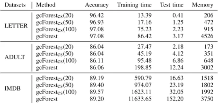
TABLE II: Comparison results (without multi-grained scanning) between gcForestcs and gcForest on accuracy (%), training time, test time (in CPU seconds) and memory usage (in megabytes). 10 test runs were conducted and the average accuracies are presented.
Datasets Method Accuracy Training time Test time Memory
LETTER gcForestcs(20) 96.42 13.39 0.41 206 gcForestcs(50) 96.93 17.16 1.25 472 gcForestcs(100) 97.08 75.23 2.23 915 gcForest 97.08 86.42 3.17 4526 ADULT gcForestcs(20) 86.04 27.47 2.18 173 gcForestcs(50) 86.04 45.19 4.12 351 gcForestcs(100) 86.11 95.48 6.86 648 gcForest 86.06 198.85 12.24 3002 IMDB gcForestcs(20) 89.19 590.79 16.63 1518 gcForestcs(50) 89.40 974.07 23.19 1802 gcForestcs(100) 89.57 1623.11 32.05 1992 gcForest 89.20 11633.65 152.20 3750
Table I shows that gcForestcs achieves comparable or even better predictive accuracy than gcForest with about an order of magnitude less memory and faster runtime. The only exception is the CIFAR-10 dataset, where the training and testing times are still 4 and 3 times faster, respectively.
Interestingly, if gcForest adopts subsampling multi-grained scanning at each level (the same as gcForestcs) instead of multi-grained scanning, its predictive accuracy will degrade heavily, e.g., it achieves 67.78% on sEMG which is much lower than the original gcForest and gcForestcs. Thus we report the results of the original gcForest only. This outcome further verifies the effectiveness of confidence screening.
B. Results without Multi-Grained Scanning
Here we conduct experiments without multi-grained scan-ning on the datasets that do not hold spatial or sequential relationships among the raw features. gcForestcs uses different numbers of trees of each forest at the first level, i.e., 20, 50 and 100 to examine their rates of improvements.
As shown in Table II, gcForestcs improves its accuracy as window size increases; but the maximal gap among them is less than 0.7%. In contrast, gcForest has a large accuracy gap, e.g., gcForest(20) achieves 88.21% on IMDB which is much lower than 89.20% achieved by gcForest(500). Because the accuracy of gcForest with fewer trees is not competitive, we report its accuracy in which each forest has 500 trees only.
Table II shows that gcForestcs(100) achieves accuracies comparable to or better than gcForest on all three datasets.
1 2 3 4 5 6 7 8 Level 9250 9500 9750 10000 10250 10500 10750
# instances Screened instances Correctly classified screened instances
(a) Screened instances
1 2 3 4 5 6 7 8 Level 3000 3500 4000 4500 5000 5500 # instances Remaining instances Correctly classified remaining instances at the current level Correctly classified remaining instances at the next level
(b) Remaining instances Fig. 4: IMDB: Screened instances and remaining instances at each level of gcForestcs. (a) The accumulated numbers of screened in-stances and correctly classified screened inin-stances up to a certain level of gcForestcs; (b) The number of remaining instances at each level of gcForestcs. At each level, the remaining instances are passed to the next level. The number of correctly classified remaining instances increases from the current level to the next level.
VI. INFLUENCE OFCONFIDENCESCREENING
In this section, we aim to study the influence of confidence screening that links the decreasing number of instances with the improvement at each level in terms of accuracy, memory and runtime. The examples are based on IMDB, and the results are similar on other datasets.
As shown in Figure 4(a), gcForestcs screens 64% of the test instances of IMDB at the first level. At the last level, only 28% test instances are passed through all the levels. In contrast, all the test instances are passed through all the levels in gcForest. The results are similar on training. This leads directly to the high reduction in memory and runtime.
We further demonstrate how confidence screening influ-ences the classification result. As Figure 4(a) shows, the accumulated number of screened instances increases as the number of levels increases. Because instances are screened if their predictions have high confidence, the accuracy of the screened instances is about 95% which is much higher than
the overall accuracy (< 90%). Interestingly, gcForestcs and
gcForest have the same predictions on the screened instances except two of them.
The result of the remaining instances is shown in Fig-ure 4(b): the blue line plots the number of remaining instances which are correctly classified at the current level; and the orange line represents the number of those correctly classified at the next level. Figure 4(b) shows that the accuracy of remaining instances increases when they are passed from the current level to the next level—due to the model used in the next level. At the final level, the number of correctly clas-sified instances of gcForestcs is 80 instances more than that of gcForest. This outcome shows that confidence screening encourages models at each level to better focus on the hard-to-predict instances that leads directly to their better hard-to-predictions.
VII. CONCLUSIONS
We propose a more efficient Deep Forest approach called gcForestcs which has significantly smaller memory require-ment and runs faster than gcForest [3]. We first identify two deficiencies of gcForest and then introduce a confidence screening mechanism to address these issues. The confidence
screening splits the instances into easy-to-predict and hard-to-predict subsets at each level of cascade, which reduces the number of instances passed to the next level. This significantly reduces the training and testing times of forests at each level. Our theoretical analysis suggests to vary the model complexity from low to high as the level increases in the cascade. This design further reduces memory requirement and time cost at the first few levels; the model complexity increases as the level increases to cope with hard-to-predict instances.
The effectiveness of the approach is validated in our eval-uation that it achieves more with less, i.e., gcForestcs has predictive accuracy comparable to or better than gcForest, with up to one order of magnitude smaller time and memory costs.
Acknowledgment: This research was supported by NSFC (61751306) and the 111 Program (B14020).
REFERENCES
[1] A. Krizhevsky, I. Sutskever, and G. E. Hinton, “Imagenet classification with deep convolutional neural networks,” in NIPS, 2012, pp. 1097– 1105.
[2] G. Hinton, L. Deng, D. Yu, G. E. Dahl, A.-r. Mohamed, N. Jaitly, A. Senior, V. Vanhoucke, P. Nguyen, T. N. Sainathet al., “Deep neural networks for acoustic modeling in speech recognition: The shared views of four research groups,”IEEE Signal Processing Magazine, vol. 29, no. 6, pp. 82–97, 2012.
[3] Z.-H. Zhou and J. Feng, “Deep forest: Towards an alternative to deep neural networks,” inIJCAI, 2017, pp. 3553–3559.
[4] L. Breiman, “Random forests,”Machine Learning, vol. 45, no. 1, pp. 5–32, 2001.
[5] F. T. Liu, K. M. Ting, Y. Yu, and Z.-H. Zhou, “Spectrum of variable-random trees,”Journal of Artificial Intelligence Research, vol. 32, pp. 355–384, 2008.
[6] Z.-H. Zhou,Ensemble Methods: Foundations and Algorithms. Boca Raton, FL: CRC, 2012.
[7] Z.-H. Zhou and J. Feng, “Deep forest: Towards an alternative to deep neural networks,”CoRR, vol. abs/1702.08835, 2017.
[8] C. Cortes, M. Mohri, and U. Syed, “Deep boosting,” inICML, 2014, pp. 1179–1187.
[9] G. DeSalvo, M. Mohri, and U. Syed, “Learning with deep cascades,” in
ALT, 2015, pp. 254–269.
[10] Y.-L. Zhang, J. Zhou, W. Zheng, J. Feng, L. Li, Z. Liu, M. Li, Z. Zhang, C. Chen, X. Li, and Z.-H. Zhou, “Distributed deep forest and its application to automatic detection of cash-out fraud,” CoRR, vol. abs/1805.04234, 2018.
[11] P. Viola and M. Jones, “Rapid object detection using a boosted cascade of simple features,” inCVPR, 2001, pp. 511–518.
[12] J. Gama and P. Brazdil, “Cascade generalization,”Machine Learning, vol. 41, no. 3, pp. 315–343, 2000.
[13] H. Zhao and S. Ram, “Constrained cascade generalization of decision trees,”IEEE Transactions on Knowledge and Data Engineering, vol. 16, no. 6, pp. 727–739, 2004.
[14] E. Nowak, F. Jurie, and B. Triggs, “Sampling strategies for bag-of-features image classification,” inECCV, 2006, pp. 490–503.
[15] F. Shi, E. Petriu, and R. Laganiere, “Sampling strategies for real-time action recognition,” inCVPR, 2013, pp. 2595–2602.
[16] K. Weinberger, A. Dasgupta, J. Langford, A. Smola, and J. Attenberg, “Feature hashing for large scale multitask learning,” inICML, 2009, pp. 1113–1120.
[17] A. Kleiner, A. Talwalkar, P. Sarkar, and M. I. Jordan, “The big data bootstrap,” inICML, 2012.
[18] L.-P. Liu, Y. Yu, Y. Jiang, and Z.-H. Zhou, “TEFE: a time-efficient approach to feature extraction,” inICDM, 2008, pp. 423–432. [19] L. V. Utkin and M. A. Ryabinin, “A siamese deep forest,”
![Fig. 2: Illustration of class vector generation from [3]. Each compo- compo-nent of the final class vector is an average of the outputs of individual trees](https://thumb-us.123doks.com/thumbv2/123dok_us/10012514.2493616/3.918.85.828.80.262/illustration-class-vector-generation-vector-average-outputs-individual.webp)