Efficient Market Making via Convex Optimization, and a
Connection to Online Learning
∗Jacob Abernethy EECS Department
University of California, Berkeley [email protected]
Yiling Chen
School of Engineering and Applied Sciences Harvard University
[email protected] Jennifer Wortman Vaughan
Computer Science Department University of California, Los Angeles
Working Draft, January 19, 2012
1Abstract
We propose a general framework for the design of securities markets over combinatorial or infinite state or outcome spaces. The framework enables the design of computationally efficient markets tai-lored to an arbitrary, yet relatively small, space of securities with bounded payoff. We prove that any market satisfying a set of intuitive conditions must price securities via a convex cost function, which is constructed via conjugate duality. Rather than deal with an exponentially large or infinite outcome space directly, our framework only requires optimization over a convex hull. By reducing the problem of automated market making to convex optimization, where many efficient algorithms exist, we arrive at a range of new polynomial-time pricing mechanisms for various problems. We demonstrate the ad-vantages of this framework with the design of some particular markets. We also show that by relaxing the convex hull we can gain computational tractability without compromising the market institution’s bounded budget. Although our framework was designed with the goal of deriving efficient automated market makers for markets with very large outcome spaces, this framework also provides new insights into the relationship between market design and machine learning, and into the complete market setting. Using our framework, we illustrate the mathematical parallels between cost function based markets and online learning and establish a correspondence between cost function based markets and market scoring rules for complete markets.
1
Introduction
Securities marketsplay a fundamental role in economics and finance. A securities market offers a set of contingent securitieswhose payoffs depend on the future state of the world. For example, an Arrow-Debreu
∗
Some of the results and text in this paper initially appeared in Chen and Vaughan [15] and Abernethy et al. [2].
1
security pays $1 if a particular state of the world is reached and $0 otherwise [5, 6]. Consider an Arrow-Debreu security that will pay off in the event that a category 4 or higher hurricane passes through Florida in 2012. A Florida resident who worries about his home being damaged might buy this security as a form of insurance to hedge his risk; if there is a hurricane powerful enough to damage his home, he will be compensated. Additionally, a risk-neutral trader who has reason to believe that the probability of a category 4 or higher hurricane landing in Florida in 2012 ispshould be willing to buy this security at any price below
por (short) sell it at any price abovepto capitalize his information. For this reason, the market price of the security can be viewed as the traders’ collective estimate of how likely it is that a powerful hurricane will occur. Securities markets thus have dual functions: risk allocationandinformation aggregation.
Insurance contracts, options, futures, and many other financial derivatives are examples of contingent se-curities. A securities market primarily focused on information aggregation is often referred to as aprediction market. The forecasts of prediction markets have proved to be accurate in a variety of domains [8, 42, 60]. While our work builds on ideas from prediction market design [4, 15, 49], our framework can be applied to any contingent securities.
A securities market is said to becompleteif it offers at least|O| −1linearly independent securities over a setOof mutually exclusive and exhaustive states of the world, which we refer to asoutcomes[5, 6, 45]. For example, a prediction market withnArrow-Debreu securities fornoutcomes is complete. In a complete securities market without transaction fees, a trader may bet on any combination of the securities, allowing him to hedge any possible risk he may have. It is generally assumed that the trader mayshort sella security, betting against the given outcome; in a market with short selling, thenth security is not strictly necessary, as a trader can substitute the purchase of this security by short selling all others. Furthermore, traders can change the market prices to reflect any valid probability distribution over the outcome space, allowing them to reveal any belief. Completeness therefore provides expressiveness for both risk allocation and information aggregation.
Unfortunately, completeness is not always achievable. In many real-world settings, the outcome space is exponentially large or even infinite. For instance, a competitive race betweennathletes results in an outcome space ofn!rank orders, while the future price of a stock has an infinite outcome space, namelyR≥0. In such
situations operating a complete securities market is not practical for two reasons: (a) humans are notoriously bad at estimating small probabilities and (b) it is computationally intractable to manage such a large set of securities. Instead, it is natural to offer a smaller set of structured securities. For example, rather than offer a security corresponding to each rank ordering, inpair bettinga market institution offers securities of the form “$1 if candidate A beats candidate B” [17, 18]. There has been a surge of recent research examining the tractability of running standard prediction market mechanisms (such as the popular Logarithmic Market Scoring Rule (LMSR) market maker [32]) over combinatorial outcome spaces by limiting the space of available securities [51]. While this line of research has led to a few positive results [3, 16, 19, 31], it has led more often to hardness results [16, 18] or to markets with undesirable properties such as unbounded loss of the market institution [24].
In this paper, we propose a general framework to designautomated market makersfor securities markets. An automated market maker is a market institution that adaptively sets prices for each security and is always willing to accept trades at these prices. Unlike previous research aimed at finding a space of securities that can be efficiently priced using an existing market maker like LMSR, we start with an arbitrary space of securities and design anewmarket maker tailored to this space. Our framework is therefore very general and includes existing market makers for complete markets, such as the LMSR and Quad-SCPM [4], as special cases.
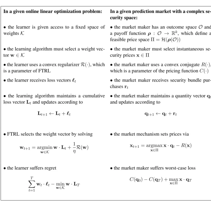
define a set of intuitive conditions that a reasonable market maker should satisfy. We prove that a market maker satisfying these conditions must price securities via a convex potential function (thecost function), and that the space of reachable security prices must be precisely the convex hull of the payoff vectors for each outcome (that is, the set of vectors, one per outcome, denoting the payoff for each security if that outcome occurs). We then incorporate ideas from online convex optimization [34, 54] to define a convex cost function in terms of an optimization over this convex hull; the vector of prices is chosen as the optimizer of this convex objective. With this framework, instead of dealing with the exponentially large or infinite outcome space, we only need to deal with the lower-dimensional convex hull. The problem of automated market making is reduced to the problem of convex optimization, for which we have many efficient techniques to leverage.
To demonstrate the advantages of our framework, we provide two new computationally efficient markets. The first market can efficiently pricesubset betson permutations, which are known to be #P-hard to price using LMSR [18]. The second market can be used to price bets on the landing location of an object on a sphere. For situations where the convex hull cannot be efficiently represented, we show that we can relax the convex hull to gain computational tractability without compromising the market maker’s bounded budget. This allows us to provide a computationally efficient market maker for the aforementioned pair betting, which is also known to be #P-hard to price using LMSR [18].
Although our framework was designed with the goal of deriving novel, efficient automated market mak-ers for markets with very large outcome spaces, this framework also provides new insights into the relation-ship between market design and machine learning, and into the complete market setting. With our frame-work, we illustrate the mathematical parallels between cost function based markets and online learning, and establish a correspondence between cost function based markets and market scoring rules for complete markets.
Roadmap of the paper The rest of the paper is organized as follows. We begin in Section 2 with a review of the relevant literature on automated market makers and prediction market design. In Section 3 we describe the problem of market design for large outcome spaces, discuss the difficulties inherent to this problem, and introduce our axiomatic approach. In Section 4 we give a detailed framework for constructing pricing mechanisms based on convex optimization and conjugate duality. We give a couple of examples of efficient duality-based cost function market makers in Section 5. In Section 6 we consider the computational issues associated with our framework, and show how the proposed convex optimization problem can be relaxed to gain tractability without increasing the worst-case loss of the market maker. We illustrate the mathematical parallels between our framework and online learning in Section 7. Finally, in Section 8, we describe how our framework can be used to establish a correspondence between cost function based markets and market scoring rules for complete markets.
2
Background and Related Work
Automated market makers for complete markets are well studied in both economics and finance. Our work builds on the literature on cost function based markets [14, 32, 33]. A simple cost function based market maker offers|O|Arrow-Debreu securities, each corresponding to a potential outcome. The market maker determines how much each security should cost using a differentiablecost function,C :R|O| →R, which is simply a potential function specifying the amount of money currently wagered in the market as a function of the number of shares of each security that have been purchased. Ifqois the number of shares of security ocurrently held by traders, and a trader would like to purchase a bundle ofroshares for each securityo∈ O (where eachro could be positive, representing a purchase, zero, or even negative, representing a sale), the
trader must payC(q+r)−C(q)to the market maker. The instantaneous price of securityo(that is, the price per share of an infinitesimal portion of a security) is then∂C(q)/∂qo, and is denotedpo(q).
One example of a cost function based market that has received considerable attention is Hanson’s Log-arithmic Market Scoring Rule (LMSR) [14, 32, 33]. The cost function of the LMSR is
C(q) =blogX o∈O
eqo/b, (1)
whereb > 0is a parameter of the market controlling the rate at which prices change. The corresponding price function for each securityois
po(q) = ∂C(q) ∂qo = e qo/b P o0∈Oeqo0/b . (2)
It is well known that the monetary loss of an automated market maker using LMSR is upperbounded by
blog|O|. Additionally, the LMSR satisfies several other desirable properties, which are discussed in more detail in Section 3.1.
When|O|is large or infinite, calculating the cost of a purchase becomes intractable in general. Recent research on automated market makers for large outcome spaces has focused on restricting the allowable securities over a combinatorial outcome space and examining whether LMSR prices can be computed effi-ciently in the restricted space. If the outcome space containsn!rank orders ofncompeting candidates, it is #P-hard to pricepair bets(securities of the form “$1 if and only if candidate A beats candidate B”) orsubset bets(for example, “$1 if one of the candidates in subsetC finishes at positionk”) using LMSR on the full set of permutations [18]. If the outcome space contains2nBoolean values ofnbinary base events, it is #P-hard to price securities on conjunctions of any two base events (for example, “$1 if and only if a Democrat wins Florida and Ohio”) using LMSR [18]. This line of research has led to some positive results when the uncertain event enforces particular structure on the outcome space. In particular, for a single-elimination tournament ofnteams, securities such as “$1 if and only if team A wins akth round game” and “$1 if and only if team A beats team B given they face off” can be priced efficiently using LMSR [19]. The tractability of these securities is due to a structure-preserving property — the market probability can be represented by a Bayesian network and price updating does not change the structure of the network. Pennock and Xia [52] significantly generalized this result and characterize all structure-preserving securities. For a taxonomy tree on some statistic where the value of the statistic of a parent node is the sum of those of its children, securities such as “$1 if and only if the value of the statistic at node A belongs to[x, y]” can be priced efficiently using LMSR [31].
One approach to combat the computational intractability of pricing over combinatorial spaces is to ap-proximate the market prices using sampling techniques. Yahoo!’s Predictalot2, a play-money combinatorial prediction market for the NCAA Men’s Basketball playoff, allows traders to bet on almost any combina-tion of the263outcomes of the tournament. Predictalot is based on LMSR. Instead of calculating the exact prices for securities, it uses importance sampling to approximate the prices. Xia and Pennock [61] devised a Monte-Carlo algorithm that can efficiently compute the price of any security in disjunctive or conjunctive normal form with guaranteed error bounds. However, using sampling techniques brings a new problem to pricing. The sampling algorithm in general won’t give the same prices if quoted twice, even if the market status remains the same. Because of this, traders can exploit the market to make a profit, which increases the loss of the market maker.
2
In this paper, we take a drastically different approach to combinatorial market design. Instead of search-ing for supportable spaces of securities for existsearch-ing market makers, we design new market makers tailored to any security space of interest and with desirable theoretical properties. Additionally, rather than requiring that securities have a fixed (e.g., $1) payoff when the underlying event happens, we allow more general contingent securities with arbitrary, efficiently computable and bounded payoffs.
Our approach makes use of powerful techniques from convex optimization. Agrawal et al. [4] and Peters et al. [53] also use convex optimization for automated market making. One major difference is that they only consider complete markets, while we consider markets with an arbitrary set of securities. They consider the setting in which traders submit limit orders, and formulate a convex optimization problem that can be solved by the market institution in order to decide what quantity of orders to accept. While formulating the problem in terms of limit orders leads to a syntactically different problem, their mechanisms can be turned into equivalent cost function based market makers. Agrawal et al. [4] show that their mechanisms can be formulated as a risk minimization problem with an associated penalty function. Mathematically the penalty function plays a similar role as the conjugate functionRin our framework, but they do not explicitly make a connection with conjugate duality.
This paper focuses on cost function based market makers. It is worth noting that there are other market mechanisms, with different properties, designed for securities markets. For complete markets, Dynamic Parimutuel Markets [44, 50] also use a cost function to price securities, however the securities are parimutuel bets whose future payoff is not fixed a priori, but depends on the market activities. Brahma et al. [10] and Das and Magdon-Ismail [21] design Bayesian learning market makers that maintain a belief distribution and update it based on the traders’ behavior. Call markets have been studied to trade securities over combinatorial spaces. In a call market, participants submit limit orders and the market institution determines what orders to accept or reject. Researchers have studied the computational complexity of operating call markets for both permutation [3, 16, 26] and Boolean [22] combinatorics.
Related work on online learning and related work on market scoring rules are discussed in Sections 7 and 8 respectively.
3
An Axiomatic Approach to Market Design
In this work, we are primarily interested in a market-design scenario in which the outcome space O is exponentially large, or even infinite, making it infeasible to run a complete market; not only is it generally intractable for the market maker to price an exponential number of securities, but it is notoriously difficult for human traders to reason about the probabilities of so many individually unlikely outcomes. To address both of these problems, we restrict the market maker to offer a menu of onlyK securities for some reasonably-sized K. These securities will be designed by the market maker and one can interpret each security as corresponding to some “interesting” or “useful” query that we might like to make about the future outcome. For example, if a set of players compete in a tournament, the market maker can offer a security for every question of the form “does playerXsurvive beyond roundY?”
We assume that the payoff of each security, clearly depending on the future outcomeo, can be described by an arbitrary but efficiently-computable functionρ:O →Rn
≥0; if a trader purchases a share of securityi
and the true outcome iso, then the trader is paidρi(o). We call such a security spacecomplex. The complete security space is a special case of a complex security space in whichK =|O|and for eachi∈ {1,· · ·, K},
ρi(o)equals 1 ifois theith outcome and0 otherwise. The markets we design enable traders to purchase arbitrarysecurity bundlesr∈RK. A negative element ofrencodes a sale of such a security. The payoff for
o. Let us defineρ(O) :={ρ(o)|o∈ O}.
The first step in the design of automated market makers for complex security spaces is to determine an appropriate set of properties that we would like such market makers to satisfy. To build intuition about which properties might be desirable, we first step back and consider what it is that makes a market maker like LMSR a good choice for complete markets.
3.1 What Makes A Market Maker Reasonable?
Consider the cost function associated with the Logarithmic Market Scoring Rule (Equation 1) and the cor-responding instantaneous price functions (Equation 2). This cost function and the resulting market satisfy several natural properties that make LMSR a “reasonable” choice.
1. The cost function is differentiable everywhere. As a result, an instantaneous price po(q) =
∂C(q)/∂qo can always be obtained for the security associated with any outcome o, regardless of the current quantity vectorq.
2. The market incorporates information from the traders, in the sense that the purchase of a security corresponding to outcomeocausespoto increase.
3. The market does not provide explicit opportunities for arbitrage. Since instantaneous prices are never negative, traders are never paid to obtain securities. Additionally, the sum of the instantaneous prices of the securities is always 1. If the prices summed to something less than (respectively, greater than) 1, a trader could purchase (respectively, short sell) small equal quantities of each security for a guar-anteed profit. This is prevented.
In addition to preventing arbitrage, these properties also ensure that prices can be interpreted naturally as probabilities, representing the market’s current estimate of the distribution over outcomes.
4. The market isexpressivein the sense that a trader with sufficient funds is always able to set the market prices to reflect his beliefs about the probability of each outcome.3
As described in Section 2, previous research on cost function based markets for combinatorial outcome spaces has focused on developing algorithms to efficiently implement or approximate LMSR pricing [18, 19, 31]. Because of this, there has been no need to explicitly extend these properties to complex markets; the properties hold automatically for any implementation of LMSR. This is no longer the case when our goal is to design new markets tailored to custom sets of securities.
To gain intuition about what makes an arbitrary complex market “reasonable,” let us begin by consid-ering the example ofpair betting[17, 18]. Suppose our outcome space consists of rankings of a set ofn
competitors, such asnhorses in a race. The outcome of such a race is a permutationπ : [n]→[n], where [n] denotes the set {1,· · · , n}, and π(i) is the final position of i, withπ(i) = 1 being best. A typical market for this setting might offernArrow-Debreu securities, with theith security paying off if and only ifπ(i) = 1. Additionally, there might be separate, independentmarkets allowing bets on horses to place (come in first or second) or show (come in first, second, or third). However, running independent markets for sets of outcomes with clear correlations is wasteful in that information revealed in one market does not automatically propagate to the others. Instead, suppose that we would like to define a set of securities that allow traders to make arbitrarypair bets; that is, for everyi, j, a trader can purchase a security which pays out $1 wheneverπ(i)< π(j). What properties would make a market for pair bets reasonable?
3
The first two properties described above have straight-forward interpretations in this setting. We would still like the instantaneous price of each security to be well-defined at all times; intuitively, the instantaneous price of the security for π(i) < π(j) should represent the traders’ collective belief about the probability that horseifinishes ahead of horse j. Call this price pi,j. We would still like the market to incorporate information, in the sense that buying the security corresponding toπ(i)< π(j)should never cause the price
pi,j to drop.
The remaining two properties are more tricky to quantify. Intuitively, these properties require us to define a set of constraints over the prices achievable in the market (to prevent arbitrage), and to ensure that any prices reflecting consistent beliefs about the distribution over outcomes can be achieved (for expressiveness). One can come up with various logical constraints that prices should satisfy. For example, pi,j must be nonnegative at all times for all iandj, andpi,j +pj,i must always equal 1 since exactly one of the two securities corresponding toπ(i) < π(j) andπ(j) < π(i)respectively will pay out $1. Similar reasoning gives us the additional constraint that for alli,j, andk,pi,j+pj,k+pk,imust be at least 1 and no more than 2. But are these constraints enough to prevent arbitrage? Are they too strong to allow the expression of arbitrary consistent beliefs?
In general, this type of ad hoc reasoning can lead us to many apparently reasonable constraints, but does not yield an algorithm to determine whether or not we have generated the full set of constraints necessary to prevent arbitrage, and cannot be applied easily to more complicated security spaces. We address this problem in the next section. We start by formalizing the desirable market properties described above in the context of complex markets. We then provide a precise mathematical characterization of all cost functions that satisfy these properties.
3.2 An Axiomatic Characterization of Complex Markets
We are now ready to formalize a set of conditions or axioms that one might expect a market to satisfy, and show that these conditions lead to some natural mathematical restrictions on the costs of security bundles. (We consider relaxations of these conditions in Section 6.) We do not presuppose a cost function based market. However, we show that the use of a convex cost function isnecessarygiven the assumption of path independence on the security purchases.
3.2.1 Path Independence and the Use of Cost Functions
Imagine a sequence of traders entering the marketplace and purchasing security bundles. Letr1,r2,r3, . . .
be the sequence of security bundles purchased. Aftert−1such purchases, thet-th trader should be able to enter the marketplace and query the market maker for the cost of arbitrary bundles. The market maker must be able to furnish a cost, denotedCost(r|r1, . . . ,rt−1), for any bundlergiven a previous trade sequence
r1, . . . ,rt−1. If the trader chooses to purchasertat a cost ofCost(rt|r1, . . . ,rt−1), the market maker may
update the costs of each bundle accordingly. Our first condition requires that the cost of acquiring a bundle
rmust be the same regardless of how the trader splits up the purchase.
Condition 1(Path Independence). For anyr,r0, andr00such thatr=r0+r00, for anyr1, . . . ,rt,
Cost(r|r1, . . . ,rt) =Cost(r0|r1, . . . ,rt) +Cost(r00|r1, . . . ,rt,r0).
Path independence helps to reduce both arbitrage opportunities and the strategic play of traders, as traders need not reason about the optimal path leading to some target position. However, it is worth pointing out that there are interesting markets that do not satisfy this condition, such as the continuous double auction
and the market maker for continuous double auctions considered by Brahma et al. [10] and Das and Magdon-Ismail [21]. These markets do not fall into our framework and deserve separate treatment.
It turns out that the path independence alone implies that prices can be represented by a cost functionC, as illustrated in the following theorem.
Theorem 1. Under Condition 1, there exists a cost functionC:RK →Rsuch that we may always write
Cost(rt|r1, . . . ,rt−1) =C(r1+. . .+rt−1+rt)−C(r1+. . .+rt−1).
Proof. LetC(q) :=Cost(q|∅). ClearlyC(0) =Cost(0|∅) = 0.We will show, via induction ont, that for anytand any bundle sequencer1, . . . ,rt,
Cost(rt|r1, . . . ,rt−1) =C(r1+. . .+rt−1+rt)−C(r1+. . .+rt−1). (3)
Whent = 1, this holds trivially. Assume that Equation 3 holds for all bundle sequences of any length
t≤T. By Condition 1, Cost(rT+1|r1, . . . ,rT) = Cost(rT+1+rT|r1, . . . ,rT−1)−Cost(rT|r1, . . . ,rT−1) = C rT+1+rT + T−1 X t=1 rt ! −C T−1 X t=1 rt ! − C rT + T−1 X t=1 rt ! −C T−1 X t=1 rt !! = C T+1 X t=1 rt ! −C T X t=1 rt ! ,
and we see that Equation 3 holds fort=T + 1too.
With this theorem in mind, we drop the cumbersome Cost(r|r1, . . . ,rt) notation from now on, and write the cost of a bundlerasC(q+r)−C(q), whereq=r1+. . .+rtis the vector of previous purchases.
3.2.2 Formalizing the Properties of a Reasonable Market
Recall that one of the functions of a securities market is to aggregate traders’ beliefs into an accurate predic-tion. Each trader may have his own (potentially secret) information about the future, which we represent as a distributionp∈∆|O|over the outcome space, where∆n={x∈Rn≥0 :
Pn
i=1xi = 1}, then-simplex. The pricing mechanism should therefore incentivize the traders to revealp, but simultaneously avoid providing arbitrage opportunities. Towards this goal, we now revisit the relevant properties of LMSR discussed in Section 3.2, and show how the ideas behind each of these properties can be extended to the complex market setting, yielding four additional conditions on our pricing mechanism.
The first condition ensures that the gradient of C is always well-defined. If we imagine that a trader can buy or sell an arbitrarily small bundle, we would like the cost of buying and selling an infinitesimal quantity of any particular bundle to be the same. If∇C(q)is well-defined, it can be interpreted as a vector of instantaneous prices for each security, with∂C(q)/∂qirepresenting the price per share of an infinitesimal amount of securityi. Additionally, we can interpret∇C(q)as the traders’ current estimates of the expected payoff of each security, in the same way that∂C(q)/∂qo was interpreted as the probability of outcomeo when considering the complete security space.
Condition 2(Existence of Instantaneous Prices). Cis continuous and differentiable everywhere onRK. The next condition encompasses the idea that the market should react to trades in a sensible way in order to incorporate the private information of the traders. In particular, it says that the purchase of a security bundlershould never cause the market to lower the price ofr. This condition is closely related to incentive compatibility for a myopic trader. It is equivalent to requiring that a trader with a distributionp∈∆|O|can never find it simultaneously profitable (in expectation) to buy a bundleror to buy the bundle−r. In other words, there can not be more than one way to express one’s information.
Condition 3(Information Incorporation). For anyqandr∈RK,C(q+2r)−C(q+r)≥C(q+r)−C(q). The no arbitrage condition states that it is never possible for a trader to purchase a security bundle r
and receive a positive profit regardless of the outcome. Without this property, the market maker would occasionally offer traders a chance to obtain a guaranteed profit, which is clearly suboptimal in terms of the market maker’s loss. However, we do consider the relaxation of this property in Section 6.
Condition 4(No Arbitrage). For allq,r∈RK, there exists ano∈ Osuch thatC(q+r)−C(q)≥r·ρ(o). Finally, the expressiveness condition specifies that any trader can set the market prices to reflect his beliefs, within anyerror, about the expected payoffs of each security if arbitrarily small portions of shares may be purchased. The approximation factor is necessary because the trader’s beliefs may only be ex-pressible in the limit.
Condition 5(Expressiveness). For anyp∈∆|O| we writexp :=Eo∼p[ρ(o)]. Then for anyp ∈∆|O|and any >0there is someq∈RKfor whichk∇C(q)−xpk< .
Having formalized our set of conditions, we must now address the question of how to determine whether or not these conditions are satisfied for a particular cost function C. The following theorem precisely characterizes the set of all cost functions that satisfy these conditions. The statement and proof require the use of a few pieces of terminology; for more on why this is necessary, see the note in Section 4. In particular, therelative boundaryof a convex setSis its boundary in the “ambient” dimension ofS. For example, if we consider then-dimensional probability simplex∆n:= {x∈Rn:Pixj = 1, xi ≥0∀i}, then the relative boundary of∆nis the set{x∈∆n:xi= 0for somei}. We use relint(S)to refer to therelative interiorof a convex setS, which is the setSminus all of the points on the relative boundary. The interior of a square in 3-dimensional space is empty, but the relative interior is not. We will use closure(S)to refer to the closure ofS, the smallest closed set containing all of the limit points ofS. For any subsetSofRd, letH(S)denote the convex hull ofS. Recall thatρ(O) :={ρ(o)|o∈ O}. Note that closure(H(ρ(O)))may not be equal to H(ρ(O))if we consider infinite spaces of outcomes or contracts.
Theorem 2. Under Conditions 2-5,Cmust be convex with
closure({∇C(q) :q∈RK}) =closure(H(ρ(O))).
Proof. We first prove convexity. AssumeCis non-convex somewhere. Then there must exist someqandr
such thatC(q)>(1/2)C(q+r) + (1/2)C(q−r). This meansC(q+r)−C(q) < C(q)−C(q−r), which contradicts Condition 3, soCmust be convex.
To prove the equality, we will establish the following two containments:
We now prove the second⊆statement. Notice that Condition 2 trivially guarantees that ∇C(q) is well-defined for anyq. To see that{∇C(q) :q∈RK} ⊆closure(H(ρ(O))), let us assume there exists someq0 for which∇C(q0)∈/ closure(H(ρ(O))). This can be reformulated in the following way: There must exists some halfspace, defined by a normal vectorr, that separates∇C(q0)from every member ofρ(O). More precisely
∇C(q0)∈/ closure(H(ρ(O))) ⇐⇒ ∃r∀o∈ O:∇C(q0)·r<ρ(o)·r.
On the other hand, lettingq := q0 −r, we see by convexity of C thatC(q+r)−C(q) ≤ ∇C(q0)·
r. Combining these last two inequalities, we see that the price of bundle r purchased with historyq is always smaller than the payoff foranyoutcome. This implies that there exists some arbitrage opportunity, contradicting Condition 4.
We finish by proving the first⊆statement. Notice thatH(ρ(O)) = {Eo∼p[ρ(o)]|p ∈ ∆|O|}which is convex, and recall that the set of derivatives{∇C(q) : q ∈ RK} of any convex functionC must form a convex set. The statement of Condition 5 is equivalent to the statement that every elementxp∈ H(ρ(O)) is a limit point of the set{∇C(q) : q ∈ RK}. But we have just established that{∇C(q) : q ∈ RK} ⊆ closure(H(ρ(O)))and thus the only case wherexpdoes not equal∇C(q)for someqis whenxplies on the relative boundary ofH(ρ(O)).
What we have arrived at from the set of proposed conditions is that (a) a pricing mechanism can always be described precisely in terms of a convex cost functionCand (b) the set of reachable prices of a mecha-nism, that is the set{∇C(q) :q∈RK}, must beidenticallythe convex hull of the payoff vectors for each outcomeH(ρ(O))except possibly differing at the relative boundary ofH(ρ(O)). For complete markets, this would imply that the set of achievable prices should be the convex hull of thenstandard basis vectors. Indeed, this comports exactly with the natural assumption that the vector of security prices in complete markets should represent a probability distribution, or equivalently that it should lie in then-simplex [4].
4
Designing the Cost Function via Conjugate Duality
The natural conditions we introduced above imply that to design a market for a set of K securities with payoffs specified by an arbitrary payoff functionρ:O →RK
≥0, we should use a cost function based market
with a convex, differentiable cost function such that closure({∇C(q) : q ∈ RK}) = closure(H(ρ(O))). We now provide a general technique that can be used to design and compare properties of cost functions that satisfy these criteria. In order to accomplish this, we make use of tools from convex analysis, and in particular, the notion ofconjugate duality. We begin by stating a precise definition of this notion of duality, as well as some useful results. We use the notation dom(f)to refer to the domain of a functionf, i.e., where it is defined and finite valued.
Definition 1(Rockafellar [56], Section 7). A convex functionf :RK →[−∞,∞]is said to beclosedwhen the epigraph off is a closed set, or equivalently, the set{x:f(x)≤α}is closed for allα∈R.
For the remainder of the paper, we will only consider closed functions.
Definition 2 (Rockafellar [56], Section 12). For any convex function f : RK → [−∞,∞], the convex conjugatef∗ off is defined as
f∗(z) := sup
x∈RK
The curious reader can find good discussions of conjugate functions in, e.g., Boyd and Vandenberghe [9] as well as Hiriart-Urruty and Lemar´echal [38]. We will cite two useful results from Rockafellar [56].
Theorem 3 (Rockafellar [56], Theorem 12.2 and Corollary 12.2.2). For any closed convex functionf : RK →[−∞,∞], the conjugatef∗is also closed and convex, andf∗∗=f. Furthermore, we can write
f∗(y) = sup
x∈relint(dom(f))
y·x−f(x).
This theorem tells us two things. First, when taking thesup, we don’t have to worry about what happens on the boundary. Second, it effectively tells us that there is a one-to-one correspondence between every closed convex function and its dual. How do various properties of the function translate when we go to the dual? We give one useful result, showing thatdifferentiabilityis a dual property tostrict convexity.
Theorem 4(Rockafellar [56], Theorem 26.3). Given a proper4closed convex functionf :RK →[−∞,∞],
f is finite and differentiable everywhere onRKif and only if its conjugatef∗is strictly convex ondom(f∗). We will use this notion of conjugate duality to aid in constructing cost functions C which satisfy our desired properties. Clearly, for any cost functionC, we can construct its conjugate, which we will henceforth refer to asR. A more interesting and useful question to examine is under what conditions we obtain a valid cost function if we constructRfirst and setC:=R∗.
Theorem 5. Assume we have an outcome spaceO and a payoff functionρsuch that ρ(O)is a bounded subset ofRK. Then for any cost functionC : RK → Rsatisfying Conditions 2-5 and whereCis closed, there exists a functionR:RK →[−∞,∞]such that
C(q) = sup
x∈relint(H(ρ(O)))
x·q−R(x). (4)
Furthermore, for any proper closed convex functionR defined onrelint(H(ρ(O))), if Ris strictly convex on its domain then the cost function defined by the conjugate,C :=R∗, satisfies Conditions 2-5.
This theorem is the key result that will guide us in designing a market pricing mechanism. This mecha-nism relies on constructing a cost functionC :RK →Rthat satisfies Conditions 2-5, and we are now given ingredients to achieve this: pickanyclosed strictly convex functionR with domain containingH(ρ(O)), and we can setC:=R∗.
Duality-based cost function market maker
Input: security spaceRKand a bounded payoff functionρ:O →RK Input: convex compact price spaceΠ(typically assumed to beH(ρ(O))) Input: closed strictly convex and differentiableRwith relint(Π)⊆dom(R)
Output: cost functionC:RK →Rdefined byC(q) := supx∈relint(Π)x·q−R(x)
Notice that in this definition, we introduce the concept of a “price space” denoted byΠ. Indeed, we will typically set the price spaceΠ =H(ρ(O)), as it is this case for which Theorem 5 holds. We give the more
4
general definition because, as we will discuss, there can be computational benefits to allowing a Πto be larger. We also require thatRbe differentiable which, while not strictly necessary, is a reasonable condition and eases the notation as we can now discuss the gradient∇R(x).
This duality based approach to designing the market mechanism is convenient for several reasons. First, it leads to markets that are efficient to implement wheneverH(ρ(O))can be described by a polynomial number of simple constraints5. The difficulty with combinatorial outcome spaces is that actually enumerat-ing the set of outcomes can be challengenumerat-ing or impossible. In our proposed framework we need only work with the convex hull of the payoff vectors for each outcome when represented by a low-dimensional payoff functionρ(·). This has significant benefits, as one often encounters convex sets which contain exponentially many vertices yet can be described by polynomially many constraints. Moreover, as the construction ofC
is based entirely on convex programming, we reduce the problem of automated market making to the prob-lem of optimization for which we have a wealth of efficient algorithms. Second, this method yields simple formulas for properties of markets that help us choose the best market to run. Two of these properties, worst-case monetary loss and worst-case information loss, are analyzed below.
A note on relative interiors and boundaries. In order to establish precise statements, our discussions about certain convex sets – e.g.{∇C},H(ρ(O)), andΠ– have required precise definitions like the relative boundary and interior, and the closure of a set. One might ask whether this is necessary, as we might be focusing too heavily on “boundary cases.” While these details are occasionally cumbersome, they are important and do arise for very simple markets. For example, for the case of a complete market on n
outcomes using the LMSR cost functionC(q) =blogP
iexp(qi/b), we have that{∇C(q) : q∈Rn}= relint(∆n); prices of 0 and 1 can be reached only in the limit.
A note on the Legendre Transformation. Given an arbitrary smooth convex functionf, we can define the Legendre Transformationwhich maps a point x ∈ dom(f) via the rule x 7→ ∇f(x). Indeed, under certain circumstances we get that this map is theinverseof the Legendre transformation of the conjugatef∗, i.e.,∇f∗(∇f(x)) =xand∇f(∇f∗(y)) =yfor everyx∈dom(f)andy∈dom(f∗). Unfortunately the latter only holds whenf is strictly convex and the interior of dom(f)is non-empty (see Rockafellar, chapter 26 [56]). So while we would like to argue that∇C is the inverse of the map∇Rfor our framework, this will generally not be true. We may still state the following useful result [56]:
C(q) =q· ∇C(q)−R(∇C(q)) for allq∈RK.
This fact is quite helpful when we recall that C(q) is defined as the supremum over x ∈ relint(Π) of
q·x−R(x). As long as∇C(q)is contained inΠ, it follows immediately that the supremum is achieved at
x=∇C(q), and by the strict convexity ofRthis solution must be unique.
4.1 Bounding Market Maker Loss and Loss of Information
We now discuss two key properties of our proposed market framework. We will make use of the notion of a Bregman divergence. TheBregman divergencewith respect to a convex functionf is given by
Df(x,y) :=f(x)−f(y)− ∇f(y)(x−y). It is clear by convexity thatDf(x,y)≥0for allxandy.
5
A convex program can be solved with arbitrarily small errorin time polynomial of1/and the size of the problem input using standard techniques such as the interior-point method. In this paper, we do not worry about finding the exact solution to the convex programs.
4.1.1 Bounding the Market Maker’s Monetary Loss
When comparing market mechanisms, it is useful to consider the market maker’s worst-case monetary loss, sup q∈RK sup o∈O (ρ(o)·q)−C(q) +C(0) .
This quantity is simply the worst-case difference between the maximum amount that the market maker might have to pay the traders (supo∈Oρ(o)·q) and the amount of money collected by the market maker (C(q)−C(0)). The following theorem provides a bound on this loss in terms of the conjugate function.
Theorem 6. Consider any duality-based cost function market maker withΠ =H(ρ(O)). The worst-case monetary loss of the market maker is no more than
sup
x∈ρ(O)
R(x)− min
x∈H(ρ(O))R(x). (5)
Furthermore, the above bound is tight, as the supremum of the market maker loss, over all quantity vectors
qand outcomeso, is exactly the value in Equation 5.
Proof. Let q denote the final vector of quantities sold, ∇C(q) denote the final vector of instantaneous prices, andodenote the true outcome. From Equation 4, we have thatC(q) =∇C(q)·q−R(∇C(q))and
C(0) =−minx∈H(ρ(O))R(x). The difference between the amount that the market maker must pay out and
the amount that the market maker has previously collected is then
ρ(o)·q−C(q) +C(0) = ρ(o)·q−(∇C(q)·q−R(∇C(q)))− min x∈H(ρ(O))R(x) = q·(ρ(o)− ∇C(q)) +R(∇C(q))− min x∈H(ρ(O))R(x) +R(ρ(o))−R(ρ(o)) = R(ρ(o))− min x∈H(ρ(O))R(x) −(R(ρ(o))−R(∇C(q))−q·(ρ(o)− ∇C(q))) (6) ≤ R(ρ(o))− min x∈H(ρ(O))R(x) −(R(ρ(o))−R(∇C(q)) −∇R(∇C(q))·(ρ(o)− ∇C(q))) = R(ρ(o))− min x∈H(ρ(O))R(x)−DR(ρ(o),∇C(q)),
whereDRis the Bregman divergence with respect toR, as defined above. The inequality follows from the first-order optimality condition for convex optimization, which says that for any convex and differentiablef
defined on the domainΠ, iffis minimized atx, then
∇f(x)·(y−x)≤0 for anyy∈Π.
Consider f(x) = R(x) −q·x. The minimum of this function occurs at x = ∇C(q) via the duality assumption. Plugging iny=ρ(o)yields the inequality.
Since the divergence is always nonnegative, this is upperbounded byR(ρ(o))−minx∈H(ρ(O))R(x),
which is in turn upperbounded bysupx∈ρ(O)R(x)−minx∈H(ρ(O))R(x).
Finally, we show that this loss bound is tight. First, select any > 0. Choose an outcomeoso that supo0∈OR(ρ(o0))−R(ρ(o)) < /2. Next, choose some q0 so that DR(ρ(o),∇C(q0)) < /2. This is
achievable because the space of gradients ofC is assumed to span relint(H(ρ(O)))via Theorem 2, and so we can ensure that∇C(q0)is arbitrarily close toρ(o). Finally, letq:=∇R(∇C(q0)), and observe that by
construction we have∇C(q) =∇C(q0). To compute the market maker’s loss for this particular choice of
qando, we apply Equation 6 to obtain:
R(ρ(o))− min x∈H(ρ(O))R(x) −(R(ρ(o))−R(∇C(q))−q·(ρ(o)− ∇C(q))) = R(ρ(o))− min x∈H(ρ(O))R(x)−DR(ρ(o),∇C(q)) > sup o0∈O R(ρ(o0))− min x∈H(ρ(O))R(x)−
where the first equality holds by the definition of the Bregman divergence, becauseq=∇R(∇C(q)).
This theorem tells us that as long as the conjugate function is bounded onH(ρ(O)), the market maker’s worst-case loss is also bounded6. It says further that this loss is actually realized, for a particular outcomeo, at least when the price vector approacheso. This suggests that loss to the market maker is worst when the traders are the most certain about the outcome.
4.1.2 Bounding Information Loss
Information loss can occur when securities are sold in discrete quantities (for example, single units), as they are in most real-world markets. Without the ability to purchase arbitrarily small bundles, traders may not be able to change the market prices to reflect their true beliefs about the expected payoff of each security, even if expressiveness is satisfied. We will argue that the amount of information loss is captured by the market’s bid-ask spread for the smallest trading unit. Given someq, the current bid-ask spread of security bundleris defined to be(C(q+r)−C(q))−(C(q)−C(q−r)). This is simply the difference between the current cost of buying the bundlerand the current price at whichrcould be sold.
To see how the bid-ask spread relates to information loss, suppose that the current vector of quantities sold isq. If securities must be sold in unit chunks, a rational, risk-neutral trader will not buy securityiunless she believes the expected payoff of this security is at leastC(q+ei)−C(q), whereeiis the vector that has value 1 at itsith element and 0 everywhere else. Similarly, she will not sell securityiunless she believes the expected payoff is at mostC(q)−C(q−ei). If her estimate of the expected payoff of the security is between these two values, she has no incentive to buy or sell the security. In this case, it is only possible to infer that the trader believes the true expected payoff lies somewhere in the range[C(q)−C(q−ei), C(q+ei)−C(q)]. The bid-ask spread is precisely the size of this range.
The bid-ask spread depends on how fast instantaneous prices change as securities are bought or sold. Intuitively, the bid-ask spread relates to the depth of the market. When the bid-ask spread is large, new purchases or sales can change the prices of the securities dramatically; essentially, the market is shallow. When the bid-ask spread is small, purchases or sales may only move the prices slightly; the market is deep. Based on this intuition, for complete markets, Chen and Pennock [14] use the inverse of∂2C(q)/∂qi2 to capture the notion of market depth for each securityiindependently. In a similar spirit, we define amarket depth parameter, β, for our complex securities markets with twice-differentiable C. Larger values of β
correspond to deeper markets. We will bound the bid-ask spread in terms of this parameter, and use this parameter to show that there exists a clear tradeoff between worst-case monetary loss and information loss; this will be formalized in Theorem 7 below.
6
In Section 6, we will state a more general, stronger bound on market maker loss capturing the intuitive notion that the market maker’s profits should be higher when the distance between the final vector of prices and the payoff vectorρ(o)of the true outcome
Definition 3. For any duality-based cost function market maker, if C is twice-differentiable, the market depth parameter β(q) for a quantity vector qis defined as β(q) = 1/Vc(q), where Vc(q) is the largest eigenvalue of∇2C(q), the Hessian ofCatq. The worst-case market depth isβ = inf
q∈RKβ(q).
Let relint(Π)be the relative interior ofΠ. IfCis twice-differentiable, then for anyqsuch that∇C(q)∈ relint(Π), we have a correspondence between the Hessian ofCatqand the Hessian ofRat∇C(q). More precisely, we have thatu>∇2C(q)u=u>∇−2R(∇C(q))ufor anyu=x−x0 withx,x0 ∈Π. (See, for example, Gorni [29] for more.) This means thatβ(q)is equivalently defined as the smallest eigenvalue of ∇2R(∇C(q))|
Π; that is, where we consider the second derivative only within the price regionΠ.
The definition of worst-case market depth implies that1/β is an upper bound on the curvature of C, which implies thatCis locally bounded by a quadratic with HessianI/β. We can derive the following.
Lemma 1. Consider a duality-based cost function market maker with worst-case market depthβ. IfC is twice differentiable, then for anyqandrwe have
DC(q+r,q)≤
krk2
2β .
Proof. Letf(t) :=DC(q+tr/krk,q). Notice thatf(0) = 0, andf0(0) = 0sinceCis differentiable and
DC(x,q)is minimized atx=qor, equivalently,f(t)is minimized att= 0. It follows thatDC(q+r,q) = Rkrk
0
Rs
0 f
00(t)dt ds by standard calculus arguments. However, f00(t) is always smaller than the largest eigenvalue of∇2C(q+tr/krk)which, by definition, is always smaller than1/β. It follows that
DC(q+r,q) = Z krk 0 Z s 0 f00(t)dt ds≤ Z krk 0 Z s 0 1 β dt ds= Z krk 0 s β ds= krk2 2β as desired.
It is easy to verify that the bid-ask spread can be written in terms of Bregman divergences. In particular,
C(q+r)−C(q)−(C(q)−C(q−r)) =DC(q+r,q) +DC(q−r,q). This implies that the worst-case bid-ask spread of a market with market depthβcan be upperbounded by a constant times1/β. That is, as the market depth parameter increases, the bid-ask spread must decrease. The following theorem shows that this leads to an inherent tension between worst-case monetary loss and information loss. Here diam(H(ρ(O))) denotes the diameter of the hull of the payoff vectors for each outcome.
Theorem 7. For any duality-based cost function market maker with worst-case market depthβ, for anyr,
qmeeting the conditions in Lemma 1, the bid-ask spread for bundlerwith previous purchasesqis no more thankrk2/β. The worst-case monetary loss of the market maker is at leastβ·diam2(H(ρ(O)))/8.
Proof. The bound on the bid-ask spread follows immediately from Lemma 1 and the argument above. The valueβlower-bounds the eigenvalues ofReverywhere onΠ. Hence, if we do a quadratic lower-bound of
Rfrom the pointx0 = arg minx∈ΠR(x)with Hessian defined byβI, then we see thatR(x)−R(x0) ≥
DR(x,x0)≥ β2kx−x0k2. In the worst-case,kx−x0k=diam(H(ρ(O)))/2, which finishes the proof.
We can see that there is a direct tradeoff between the upper bound7of the bid-ask spread, which shrinks asβgrows, and the lower bound of the worst-case loss of the market maker, which grows linearly inβ. This
7
Strictly speaking, as we are emphasizing the necessary tradeoff between bid-ask spread and worst-case loss, we should have a
lower boundon the bid-ask spread. On the other hand, if the worst-case market depth parameter isβthen there is someqandr
such thatDC(q+r,q)/krk2≈1/(2β)and this approximation can be made arbitrarily tight for small enoughrwhenCis twice
tradeoff is very intuitive. When the market is shallow (smallβ), small trades have a large impact on market prices, and traders cannot purchase too many shares of the same security without paying a lot. When the market is deep (largeβ), prices change slowly, allowing the market maker to gain more precise information, but simultaneously forcing the market maker to take on more risk since many shares of a security can be purchased at prices that are potentially too low. This tradeoff can be adjusted by scalingR, which scalesβ. This is analogous to adjusting the “liquidity parameter”bof the LMSR.
4.2 Selecting a Conjugate Function
We have seen that the choice of the conjugate functionRimpacts market properties such as worst-case loss and information loss. We now explore this choice in more detail.
In many situations, the ideal choice of the conjugate is a function of the form
R(x) := λ
2kx−x0k
2. (7)
Here R(x) is simply the squared Euclidean distance between x and an initial price vector x0 ∈ Π,
scaled by λ/2. By utilizing this quadratic conjugate function, we achieve a market depth that is uni-formly λ over the entire security space. Furthermore, if x0 is chosen as the “center” of Π, namely
x0 = arg minx∈Πmaxy∈Πkx−yk, then the worst-case loss of the market maker is maxx∈ΠR(x) =
(λ/8)diam2(Π). While the market maker can tune λappropriately according to the desired tradeoff be-tween worst-case market depth and worst-case loss, the tradeoff is tightest when R has a Hessian that is uniformly a scaled identity matrix, or more precisely whereRtakes the form in Equation 7.
Unfortunately, by selecting a conjugate of this form, or any R with bounded derivative, the market maker does inherit one potentially undesirable property: security prices may become constant when∇C(q) reaches a point at relbnd(Π), the relative boundary of Π(see Section 4.1). That is, if we arrive at a total demandqwhere∇C(q) = ρ(o)for some outcomeo, our mechanism begins offering securities at a price equal to the best-case payoff, akin to asking someone to bet a dollar for the chance to possibly win a dollar. The Quad-SCPM for complete markets is known to exhibit this behavior [4].
To avoid these undesirable pricing scenarios, it is sufficient to require that our conjugate function satisfies one condition. We say that a convex functionRdefined onΠis apseudo-barrier8forΠifk∇R(xt)k → ∞ for any sequence of points x1,x2, . . . ∈ Π which tends towards relbnd(Π). If we require our conjugate
functionRto be a pseudo-barrier, we are guaranteed that the instantaneous price vector∇C(q)always lies in relint(Π), and does not become constant near the boundary.
It is important to note that, while it is desirable that k∇R(xt)k → ∞asxt approaches relbnd(Π), it is generally not desirable thatR(xt) → ∞. Recall that the market maker’s worst-case loss grows with the maximum value of R onΠ and thus we should hope for a conjugate function that is bounded on the domain. A perfect example of convex function that is simultaneously bounded and a pseudo-barrier is the negative entropy functionH(x) =P
ixilogxi, defined on then-simplex∆n. It is perhaps no surprise that LMSR, the most common market mechanism for complete security spaces, can be described by the choice
R(x) :=bH(x)where the price spaceΠ = ∆n[4, 15].
8
We use the term pseudo-barrier to distinguish this from the typical definition of a barrier function on a setΠ, which is a function that grows without bound towards the boundary ofΠ. The termLegendrewas introduced by Cesa-Bianchi and Lugosi [13] for a similar notion, yet their definition requires the stronger condition thatΠcontain a nonempty interior.
5
Examples of Computationally Efficient Markets
In the previous section, we provided a general framework for designing markets on combinatorial or infinite outcome spaces. We now provide some examples of markets that can be operated efficiently using this framework.
5.1 Subset Betting
Recall the scenario described in Section 3.1 in which the outcome is a ranking of a set of ncompetitors, such asnhorses in a race, represented as a permutationπ : [n]→ [n]. Chen et al. [17] proposed a betting language,subset bettingin which traders can place bets(i, j), for any candidateiand any slotj, that pay out $1 in the event thatπ(i) =jand $0 otherwise.9 Chen et al. [18] showed that pricing bets of this form using LMSR is #P-hard and provided an algorithm for approximating the prices by exploiting the structure of the market. Using our framework, it is simple to design a computationally efficient market for securities of this form.
In order to set up such a combinatorial market within our framework, we must be able to efficiently work with the convex hull of the payoff vectors for each outcome. Notice that, for an outcomeπ, the associated payoff can be described by a matrixMπ, withMπ(i, j) =I[π(i) =j], whereI[·]is the indicator function. Taking this one step further, it is easy to verify that the convex hull of the set of permutation matrices is precisely the set ofdoubly stochastic matrices, that is the set
Π = X ∈Rn≥×0n : n X i0=1 X(i0, j) = n X j0=1 X(i, j0) = 1 ∀i, j ,
whereX(i, j)represents the element at theith row andjth column of the matrixX. Notice, importantly, that this set is described by onlyn2variables andO(n)constraints.
To fully specify the market maker, we must also select a conjugate function R for our price space. While the quadratic conjugate function is an option, there is a natural extension of the entropy function, whose desirable properties were discussed in the previous section, for the space of stochastic matrices. For anyX ∈Π, let us set
R(X) =λX
i,j
X(i, j) logX(i, j).
The worst-case market depth is computed as the minimum of the smallest eigenvalue of the Hessian ofR
within the relint(Π). This occurs at the matrix with all values1/n, hence the worst-case depth isnλ. The worst-case loss, on the other hand, is easily computed asλnlogn.
5.2 Sphere Betting
One important challenge of operating a combinatorial prediction market is to always maintain the logical consistency of security prices. Our framework offers a way to incorporate the constraints on security prices into pricing. Hence, in addition to combinatorial prediction markets, our framework can be used to design markets where security prices have some natural constrains due to their problem domains.
9
The original definition of subset betting allowed bets of the form “any candidate in setSwill end up in slotj” or “candidate
iwill end up in one of the slots in setS.” A bet of this form can be constructed easily using our betting language by bundling multiple securities.
We consider an example in which the outcome space is infinite. An object orbiting the planet, perhaps a satellite, is predicted to fall to earth in the near future and will land at an unknown location, which we would like to predict. We represent locations on the earth as unit vectorsu ∈ R3. The difficulty of this example arises from the fact that the outcome must be a unit vector, imposing constraints on the three coordinates. We will design a market with three securities, each corresponding to one coordinate of the final location of the object. In particular, securityiwill pay off ui + 1dollars if the object lands in location u. (The addition of1, while not strictly necessary, ensures that the payoffs, and therefore prices, remain positive, though it will be necessary for traders to sell securities to express certain beliefs.) This means that traders can purchase security bundlesr∈R3and, when the object lands at a locationu, receive a payoff(u+1)·r. Note that in this example, the outcome space is infinite, but the security space is small.
The price space H(ρ(O)) for this market will be the 2-norm unit ball centered at1. To construct a market for this scenario, let us make the simple choice ofR(x) = λkx−1k2 for some parameterλ > 0.
Whenkqk ≤2λ, there exists anxsuch that∇R(x) =q. In particular, this is true forx= (1/2)q/λ+1, andq·x−R(x)is minimized at this point. Whenkqk > 2λ,q·x−R(x) is minimized at anxon the boundary ofH(ρ(O)). Specifically, it is minimized atx=q/||q||+1. From this, we can compute
C(q) = ( 1
4λkqk
2+q·1, whenkqk ≤2λ,
kqk+q·1−λ, whenkqk>2λ.
The market depth parameterβ is2λ; in fact,β(x) = 2λfor any price vectorxin the interior ofH(ρ(O)). By Theorem 6, the worst-case loss of the market maker is no more thanλ, which is precisely the lower bound implied by Theorem 7. Finally, the divergenceDC(q+r,q)≤ krk2/(4λ)for allq,r, with equality whenkqk,kq+rk ≤2λ, implying that the bid-ask spread scales linearly withkrk2/λ.
We note that for this particular prediction problem, if we try to predict the latitude and longitude of the landing location, we don’t have any constraints on prices. In particular, we can have two securities that pay off linearly with the latitude and longitude of the landing location respectively. These two securities are independent and can be traded in two independent markets.
6
Computational Complexity and Relaxations
In Section 3, we argued that the space of feasible price vectors should be preciselyH(ρ(O)), the convex hull of the payoff vectors for each outcome. In each of our examples, we have discussed market scenarios for which this hull has a polynomial number of constraints, allowing us to efficiently set prices via convex optimization. Unfortunately, one should not necessarily expect that a given payoff function and outcome space will lead to an efficiently describable convex hull. In this section, we explore a couple of approaches to overcome such complexity challenges. First, we discuss the case in whichH(ρ(O))has exponentially (or infinitely) many constraints yet gives rise to aseparation oracle. Second, we show that the price spaceΠ can indeed berelaxed beyondH(ρ(O))without increasing the risk to the market maker. Finally, we show how this relaxation applies in practice.
6.1 Separation Oracles
If we encounter a convex hullH(ρ(O))with exponentially-many constraints, all may not be lost. Recall that, in order to set prices, we need to solve the optimization problemmaxx∈H(ρ(O))q·x−R(x). Under
Consider a convex optimization problem with a concave objective functionf(x)and constraintsgi(x)≤ 0for alliin some index setI. That is, we want to solve:
max f(x) s.t. x∈Rd
gi(x)≤0∀i∈I
This can be converted to a problem with a linear objective in the standard way: max c
s.t. x∈Rd, c∈R
f(x)≥c
gi(x)≤0∀i∈I
Of course, ifIis an exponentially or infinitely large set we will have trouble solving this problem directly. On the other hand, the constraint set may admit an efficient separation oracle, defined as a function that takes as input a point (x, c) and returns trueif all the necessary constraints are satisfied or, otherwise, returns false andspecifies a violated constraint10. Given an efficient separation oracle one has access to alternative methods for optimization, the most famous being Khachiyan’sellipsoid method, that run in polynomial time. For more details see, for example, Gr¨otschel et al [30].
This suggests that a fruitful direction for designing computationally efficient market makers is to exam-ine the pricing problem on an instance-by-instance basis, and for a particular instance of interest, leverage the structure of the instance to develop an efficient algorithm for solving the specific separation problem. We leave this for future research.
6.2 Relaxation of the Price Space
When dealing with a convex hullH(ρ(O))that has a prohibitively large constraint set and does not admit an efficient separation oracle we still have one tool at our disposal: we can modifyH(ρ(O))to get an alternate price spaceΠwhich wecanwork with efficiently. Recall that in Section 3, we arrived at the requirement thatΠ = H(ρ(O))as a necessary conclusion of the proposed conditions on our market maker. If we wish to violate this requirement, we need to consider which conditions must be weakened and revise the resulting guarantees from Section 3.
We will continue to construct our markets in the usual way, via the tuple (O,ρ,Π, R) whereOis the outcome space,ρis the payoff function,Π⊆Rdis a convex compact set of feasible prices, andR :Rd→R is a strictly convex function with domainΠ. The market’s cost functionCwill be the conjugate ofRwith respect to the set Π, as in Equation 4. The only difference is that we now allow Π to be distinct from H(ρ(O)). Not surprisingly, the choice of Π will affect the interest of the traders and the market maker. We prove several claims which will aid us in our market design. Theorem 8 tells us that the expressiveness condition should not be relaxed, while Theorem 9 tells us that the no-arbitrage condition can be. Together, these imply that we may safely chooseΠto be asupersetofH(ρ(O)).
Theorem 8. For any duality-based cost function market maker, the worst-case loss of the market maker is unbounded ifρ(O)*Π.
10
Proof. Consider some outcomeosuch thatρ(o)∈/ Π. The feasible price setΠ ={∇C(q) :∀q}is compact. Becauseρ(o)∈/ Π, there exists a hyperplane thatstronglyseparatesΠandρ(o). In other words, there exists ank >0such that||ρ(o)− ∇C(q)|| ≥k,∀q.
When outcomeois realized,B(q) =ρ(o)·q−C(q) +C(0)is the market maker’s loss givenq. We have∇B(q) =ρ(o)− ∇C(q), which represents the instantaneous change of the market maker’s loss. For infinitesimal, letq0 =q+(ρ(o)− ∇C(q)). Then
B(q0) = B(q) +∇B(q)·[(ρ(o)− ∇C(q))] = B(q) +||ρ(o)− ∇C(q)||2≤B(q) +k2.
This shows that for anyqwe can find aq0such that the market maker’s worst-case loss is at least increased by k2. This process can continue for infinite steps. Hence, we conclude that the market maker’s loss is unbounded.
This (perhaps surprising) theorem tells us that expressiveness is not only useful for information aggre-gation, it is actuallynecessaryfor the market maker to avoid unbounded loss. The proof involves showing that ifois the final outcome andρ(o) 6∈ Π, then it is possible to make an infinite sequence of trades such that each trade causes a constant amount of loss to the market maker.
In the following theorem, which is a simple extension of Theorem 6, we see that including additional price vectors inΠdoes not adversely impact the market maker’s worst-case loss, despite the fact that the no-arbitrage condition is violated.
Theorem 9. Consider any duality-based cost function market maker with R and Π satisfying supx∈H(ρ(O))R(x) < ∞ and H(ρ(O)) ⊆ Π. Assume that the initial price vector satisfies ∇C(0) ∈
H(ρ(O)). Letqdenote the vector of quantities sold andodenote the true outcome. The monetary loss of the market maker is no more than
R(ρ(o))− min
x∈H(ρ(O))R(x)
−DR(ρ(o),∇C(q)).
Proof. This proof is nearly identical to the proof of Theorem 6. The only major difference is that now
C(0) = −minx∈ΠR(x) instead ofC(0) = −minx∈H(ρ(O))R(x), but this is equivalent since we have
assumed that ∇C(0) ∈ H(ρ(O)). R(ρ(o)) is still well-defined and finite since we have assumed that H(ρ(O))⊆Π.
This tells us that expanding Π can only help the market maker; increasing the range of ∇C(q) can only increase the divergence term. This may seem somewhat counterintuitive. We originally required that Π ⊆ H(ρ(O)) as a consequence of the no-arbitrage condition, and by relaxing this condition, we are providing traders with potential arbitrage opportunities. However, these arbitrage opportunities do not hurt the market maker. As long as the initial price vector lies inH(ρ(O)), any such situations where a trader can earn a guaranteed profit are effectively created (and paid for) by other traders! In fact, if the final price vector ∇C(q)falls outside the convex hull, the divergence term will be strictly positive, improving the bound.
To elaborate on this point, let’s consider an example whereΠis strictly larger thanH(ρ(O)). Letqbe the current vector of purchases, and assume the associated price vectorx = ∇C(q)lies in the interior of H(ρ(O)). Consider a trader who purchases a bundlersuch that the new price vector leaves this set, i.e.,
y:= ∇C(q+r)∈ H/ (ρ(O)). We claim that this choice can be strictly improved in the sense that there is an alternative bundler0whose associated profit, for any outcomeo, is strictly greater than the profit forr.
For simplicity, assume y is an interior point of Π \ H(ρ(O)) so that q + r = ∇R(y). Define
π(y) := arg miny0∈H(ρ(O))DR(y0,y), the minimum divergence projection ofyinto H(ρ(O)). The
al-ternative bundle we consider isr0 =∇R(π(y))−q. Our trader paysC(q+r)−C(q+r0)less to purchase
r0than to purchaser. Hence, for any outcomeo, we see that the increased profit forr0overris
ρ(o)·(r0−r)−C(q+r0) +C(q+r) > ρ(o)·(r0−r) +∇C(q+r0)·(r−r0)
= (ρ(o)−π(y))·(r0−r). (8)
Notice that we achieve strict inequality precisely because∇C(q+r0) = π(y) 6=y = ∇C(q+r). Now use the optimality condition forπ(y) to see that, sinceρ(o) ∈ H(ρ(O)),∇π(y)(DR(π(y),y))·(ρ(o)−
π(y)) ≥ 0. It is easy to check that ∇π(y)(DR(π(y),y)) = ∇R(π(y))− ∇R(y) = r0−r. Combining this last expression with the inequality above and (8) tells us that the profit increase is strictly greater than (ρ(o)−π(y))·(r0−r)≥0. Simply put, the trader receives a guaranteed positive increase in profit for any outcomeo.
The next theorem shows that any time the price vector lies outside of ρ(o), traders could profit by moving it back inside. The proof uses a nice application of minimax duality for convex-concave functions.
Theorem 10. For any duality-based cost function market maker, given a current quantity vectorq0 with
current price vector ∇C(q0) = x0, a trader has the opportunity to earn a guaranteed profit of at least
minx∈H(ρ(O))DR(x,x0).
Proof. A trader looking to earn a guaranteed profit when the current quantity is q0 hopes to purchase a
bundlerso that the worst-case profitmino∈Oρ(o)·r−C(q0+r) +C(q0)is as large as possible. Notice
that this quantity is strictly positive sincer = 0, which always has 0 profit, is one option. Thus, a trader would like to solve the following objective:
max r∈RK min o∈Oρ(o)·r−C(q0+r) +C(q0) = min x∈H(ρ(O))rmax∈RK x·r−C(q0+r) +C(q0) = min x∈H(ρ(O))rmax∈RKx·(q0+r)−C(q0+r) +C(q0)−x·q0 = min x∈H(ρ(O))R(x) +C(q0) −x·q0 = min x∈H(ρ(O))R(x) +x0 ·q0−R(x0)−x·q0 ≥ min x∈H(ρ(O))DR(x,x0).
The first equality with themin/maxswap holds via Sion’s Minimax Theorem [59]. The last inequality was obtained using the first-order optimality condition of the solutionx0 = arg maxx∈Πx·q0−R(x)for the
vectorx−x0which holds sincex∈Π.
Whenx0 ∈ H(ρ(O)),DR(x,x0)is minimized whenx= x0 and the bound is vacuous, as we would
expect. The more interesting case occurs when the prices have fallen outside ofH(ρ(O)), in which case a trader is guaranteed a riskless profit by moving∇C(q)to the closest point inH(ρ(O)).
6.3 Pair Betting via Relaxation
We return our attention to the scenario where the outcome is a ranking ofncompetitors, as described in Section 3.1. Consider a complex market in which traders make arbitrary pair bets: for everyi, j, a trader