econstor
www.econstor.eu
Der Open-Access-Publikationsserver der ZBW – Leibniz-Informationszentrum WirtschaftThe Open Access Publication Server of the ZBW – Leibniz Information Centre for Economics
Nutzungsbedingungen:
Die ZBW räumt Ihnen als Nutzerin/Nutzer das unentgeltliche, räumlich unbeschränkte und zeitlich auf die Dauer des Schutzrechts beschränkte einfache Recht ein, das ausgewählte Werk im Rahmen der unter
→ http://www.econstor.eu/dspace/Nutzungsbedingungen nachzulesenden vollständigen Nutzungsbedingungen zu vervielfältigen, mit denen die Nutzerin/der Nutzer sich durch die erste Nutzung einverstanden erklärt.
Terms of use:
The ZBW grants you, the user, the non-exclusive right to use the selected work free of charge, territorially unrestricted and within the time limit of the term of the property rights according to the terms specified at
→ http://www.econstor.eu/dspace/Nutzungsbedingungen By the first use of the selected work the user agrees and declares to comply with these terms of use.
zbw
Leibniz-Informationszentrum Wirtschaft Hager, Svenja; Schöbel, RainerWorking Paper
A note on the correlation smile
Tübinger Diskussionsbeitrag, No. 297Provided in cooperation with:
Eberhard Karls Universität Tübingen
Suggested citation: Hager, Svenja; Schöbel, Rainer (2005) : A note on the correlation smile, Tübinger Diskussionsbeitrag, No. 297, urn:nbn:de:bsz:21-opus-21079 , http:// hdl.handle.net/10419/40330
A Note on the Correlation Smile
Svenja Hager and Rainer Schöbel
∗First Version: May 2005
This Version: December 2005
Abstract
The correct modeling of default dependence is essential for the valuation of multi-name credit derivatives. However for the pricing of synthetic CDOs a one-factor Gaussian copula model with constant and equal pairwise correlations, default intensities and recovery rates for all assets in the reference portfolio has become the standard market model. If this model were a reflection of market opinion there wouldn’t be the implied correlation smile that is observed in the market. The purpose of this paper is to explain the structure of the smile by discussing the influence of different correlation matrices on CDO spreads.
JEL Classification: G13
Keywords: default risk, CDOs, implied correlation smile, correlation matrix, hetero-geneity
1
Introduction
In 2003, default swaps on the Trac-X and Dow Jones iBoxx portfolios were introduced. Tranches linked to these reference sets also started to be actively quoted. A more liquid and transparent market for tranched credit risk evolved from this portfolio stan-dardization. The recent merger of the Trac-X and Dow Jones iBoxx to the Dow Jones iTraxx in Europe and the Dow Jones CDX in the US drove this process even further. The new liquidity of the market led increasingly to the quotation of tranched products in terms of an implied correlation parameter instead of the quotation in terms of the spread or the price of a tranche. This practice is well known from the use of implied volatilities in options markets. The implied compound correlation of a tranche is the uniform asset correlation that makes the tranche spread computed by the standard market model equal to its observed market spread. The standard market model is a Gaussian copula model that uses only one single parameter to summarize all correla-tions among the various borrowers’ default times. Moreover the model assumes that
∗Department of Corporate Finance, Faculty of Economics and Business Administration,
not only pairwise correlations but also recovery rates and CDS spreads are constant and equal. An obvious advantage of this approach is its simplicity. This might be the main reason why it is used extensively in the market. But particularly a flat corre-lation structure is not sufficient to reflect the heterogeneity of the underlying assets accordingly since the complex relationship between the default times of different as-sets can’t be expressed in one single number. For that reason it is not appropriate to use implied correlations of traded tranches to price off-market tranches with the same underlying or to use implied correlations for relative value considerations (when comparing alternative investments in CDO tranches). Mashal et al. (2004) show that the use of this quotation device may lead to wrong relative value assessments because the real dependence structure of the underlying is neglected. Moreover implied corre-lations suffer from both existence and uniqueness problems. Tranche spreads are not necessarily monotone in correlation, and we may observe market prices that are not attainable by a choice of correlation. Another drawback of the use of implied corre-lations is the observed correlation smile. Quotations available in the market indicate that different tranches on the same underlying portfolio trade at different implied cor-relations. If the standard market model described market prices correctly the implied default correlation would trivially be constant over tranches. There are several reasons for the market prices not being consistent with the standard market model and for the implied correlation smile appearing in the market. On the one hand the model makes the simplifying assumption that recovery rates and CDS spreads are constant and equal for all obligors. Therefore the skew may be a consequence of these assumptions and of the assumed independence of default intensities and recovery rates. It may also be due to an incorrect specification of the dependence structure. On the other hand it is well known that the Gaussian copula overestimates the chance of observing just a few defaults and underestimates the chance of observing a very high or a very low number of defaults. Thus the Gaussian copula model may not accurately reflect the joint distribution of default times. Finally supply and demand imbalances may play a role since mezzanine tranches are extremely popular with investors.
Recently more and more researchers examine different approaches to explain and model the correlation smile. Gregory and Laurent (2004) present an extension to the Gaus-sian one-factor copula model1that allows a clustered correlation structure by specifying
inter and intra sector correlation. Additionally they introduce dependence between re-covery rates and default events which leads to an improved modeling of the smile. Unfortunately, introducing additional factors leads to exponentially increasing compu-tational time. Hull and White (2004) evaluate the sensitivity of CDO spreads to a variety of parameters like default probability, recovery rate and correlation. To ex-plain the observed correlation smile they discuss the effect of uncertain recoveries on the specification of the smile. Andersen and Sidenius (2004) also extend the Gaussian one-factor model by randomizing recovery rates. In addition they allow for correlation between recovery rates and defaults. In a second extension they introduce random factor loadings (two point distribution) to permit higher correlation in economic de-pressions. Both approaches are able to model a smile. Tavares et al. (2004) propose
1In the one-factor model a latent factor drives dependence between default times. Conditionally
on this factor the assets are independent. See Laurent and Gregory (2003) for a detailed discussion about the pricing of basket credit derivatives and synthetic CDO tranches in the one-factor model.
a composite basket model to deal with the Gaussian copula smile. They combine the copula model (to model the default risk that is driven by the economy) with indepen-dent Poisson processes (to model the default risk that is driven by a particular sector and by the company in question).
Sometimes base correlations are quoted instead of tranche correlations. The base cor-relation for a certain enhancement level is the constant pairwise corcor-relation that makes the total value of all tranches up to and including the current tranche equal to zero. For instance in case of the DJ iTraxx Europe 5yr index, the 0% to 9% base correlation is the correlation that causes the sum of the values of the 0% to 3%, the 3% to 6% and the 6% to 9% tranches to be zero. McGinty et al. (2004) discuss this subject. They explain how base correlations may facilitate the valuation of tranches with the same collateral pool that are not traded actively. They point out that there is only one base correlation for a special detachment point and that it is a much smoother line than the implied correlation. Nonetheless we observe skews. Willemann (2004) shows that even if the base correlation setup offers some benefits over the traditional compound correlation approach it should be interpreted and used carefully. He shows that even if the true default correlation increases, base correlations for some tranches may actually decrease. Furthermore base correlations are only unique given the set of attachment points. This means that across the North American and European markets, base cor-relations will be different because the tranche structures are not the same. Kamat and Oks (2004) exemplify that using a full correlation matrix instead of one number has a fat tail effect. This effect can cause higher spreads for mezzanine and senior tranches and can therefore influence the base correlation skew.
The purpose of this paper is to assess the importance of the dependence structure regarding the valuation of CDO tranches. We discuss whether a heterogeneous in-terdependence structure can be the reason for the observed correlation smile. We consider a portfolio with constant and equal default time intensities and constant and equal recovery rates and assume that the dependence between the assets is created by a Gaussian copula. We use the Gaussian copula model because it is the current indus-try standard. We choose different correlation matrices, compute the tranche spreads and derive the implied correlations. Depending on the chosen correlation structure we observe different forms of smiles. In our setup the resulting smile is solely due to the correlation matrix. We find that neglecting the actual correlation between default times results in a correlation smile and that a full correlation matrix might consequently be capable of explaining the smile.
The paper is organized as follows: The second section presents the pricing of syn-thetic CDOs. The intensity based approach that models default times is considered. We use the Gaussian copula model to introduce the dependence structure between default times. Furthermore we present the Monte Carlo simulation technique to com-pute CDO tranche spreads. The third section deals with the correlation smile that is observed in the market. We exemplify the influence of different correlation matrices on the smile. The last section concludes.
2
Pricing of Synthetic CDOs
2.1
Modeling of Default Times
We consider one asset with associated default time τ. Let N(t) be a Poisson process with intensity λ.
Definition (Poisson Process)
A Poisson process with intensity λ > 0 is a non-decreasing integer-valued process with initial value N(0) = 0. The increments of N(t) are independent and satisfy
P(N(T)−N(t) =n) = n!1(T −t)nλnexp{−(T −t)λ} for all 0≤t < T.
The time of defaultτ is the time of the first jump of N(t), i.e. τ = inf{t ∈R+|N(t)>
0}. Consequently the survival probability is P(τ > t) = exp{−λt}. Since τ de-notes a random variable with continuous distribution function F(t) = P(τ ≤ t) = 1−exp{−λt}, the random variablesF(τ)and 1−F(τ) have uniform distributions on [0,1]. This allows to simulate default times in the following way: Let U be a uniform random variable. Default times can be defined by τ ={t ∈R+|t =−ln(U)
λ }.
Indepen-dence of uniform random variables Ui and Uj implies independence of default times
τi and τj. The setup can be extended such that the intensity λ follows a stochastic
process. Stochastic intensities account for the dynamics of the credit spreads observed in the market.
2.2
The Gaussian Copula Model for Dependent Defaults
In the following we considernassets with associated random default timesτ1, ..., τnand
intensities λ1, ..., λn. The unconditional marginal distribution of the default time τi is
Fi(t) = P(τi ≤ t) = 1−exp{−λit}. Correlated defaults are modeled in the following
way: LetX1, ..., Xn be standard Gaussian random variables with distribution function
Φand correlation matrixΣ. The uniformly distributed stochastic threshold mentioned above can be defined asUi = 1−Φ(Xi). Then we obtain default times asτi =Fi−1(Ui).
The dependence structure between the assets is modeled by a Gaussian copula function
CΣn. The joint distribution of τ1, ..., τn is therefore
F(t1, ..., tn) = P(τ1 < t1, ..., τn< tn) =CΣn(F1(t1), ..., Fn(tn)).
Apparently the full correlation matrix Σ contains many parameters to fit. The curse of dimensionality can sometimes be reduced by assuming that only one latent factor drives the dependence between default times. This assumption leads to a restriction of the correlation structure but in many cases the one-factor model has sufficient degrees of freedom to replicate market prices.
2.3
Valuation of CDO Tranche Spreads
A synthetic CDO can be compared with a default swap transaction because the CDO margin payments are exchanged with the default payments on the tranche. The pre-mium X is derived by setting the margin payments and the default payments equal. Following Laurent and Gregory (2003) we consider a synthetic CDO whose underlying
consists of n reference assets and assume that asset j has exposure Ej and loss given
default Rj. Nj(t) = 1{τj≤t} denotes the default indicator process. The cumulative portfolio loss at time t is therefore L(t) = Pn
j=1RjEjNj(t). A CDO is a structured
product that can be divided into various tranches. The spread of a tranche with a certain enhancement level depends on the thresholdsAand B,0≤A < B ≤Pn
j=1Ej.
The cumulative default of tranche (A, B) is the non-decreasing function
ω(L(t)) = (L(t)−A)1[A,B](L(t)) + (B−A)1]B,Pn
j=1RjEj](L(t)).
LetB(t)be the discount factor for maturity t. T stands for the maturity of the CDO and t1, ..., tI denote the regular payment dates for the CDO margins.
The default payments can be written as
E " n X j=1 B(τj)Nj(T)(ω(L(τj))−ω(L(τj−))) # .
The margin payments are based on the outstanding nominal of the tranche. Since defaults often take place between regular payment dates we have to distinguish between the regular payments
X
I
X
i=1
B(ti)E[ω(∞)−ω(L(ti))]
and the accrued payments. Accrued margins are paid for the time from the last regular payment date before τj (this date is calledtk(j)−1) until τj.
XE " n X j=1 B(τj)Nj(T)(τj−tk(j)−1)(ω(L(τj))−ω(L(τj−))) #
Since there is no closed-form solution for the portfolio loss distribution CDO margins generally have to be computed by Monte Carlo simulations. Substantial simplifications can be achieved by using a factor model. In the one-factor approach semi-explicit expressions can be provided for the pricing of synthetic CDOs.
2.4
Monte Carlo Simulation of CDO Tranche Spreads
We assume a homogeneous CDO. All obligors have the same notional E, the same loss given defaultR and the same default intensityλ. Using these assumptions we can simplify the cumulative portfolio loss at time t toL(t) = REPn
j=11{τj≤t}.
Before we estimate the portfolio loss at time t we have to simulate the default dates. At first we sample a set of n correlated uniform random variates. This is done by specifying a copula function, which is a probability distribution function defined on the n-dimensional unit cube. We choose the Gaussian copula CΣn with correlation matrix Σand follow the below-mentioned algorithm.
1. Find the Cholesky decomposition A of Σ.
2. Simulatenindependent standard normally distributed random variatesz= (z1, ..., zn).
3. Set x=Az. Then x is multivariate normal with mean zero and correlation matrix Σ.
4. Set ui = 1−Φ(xi) where Φ denotes the univariate standard normal distribution.
Then we have (1−u)∼Cn
Σ for u= (u1, ..., un).
5. The default dates can now be derived from the uniform random variates. They are given by τi =−ln(uλi), i= 1, ..., n.
Using the simulated correlated default dates we can now calculate the loss at time
t. The kth simulation gives Lk(t). Repeat steps 1 to 5 m times. The estimator for
the cumulative loss is then L(t) = m1 Pm
k=1Lk(t). In the following we compute CDO
spreads withm = 100000 iterations. This yields a standard error of less than 2%.
3
The Correlation Smile
The implied correlation of a certain tranche is the uniform asset correlation that makes the spread of this tranche as computed according to the standard Gaussian copula model equal to the observed market spread. It is increasingly applied when comparing different investments in synthetic CDO tranches. Besides implied correlations of traded tranches are used to value off-market tranches with the same underlying. However rel-ative value considerations or valuations of off-market tranches by means of the implied correlation can be misleading. The observed correlation smile shows that using a flat correlation matrix can result in severe mispricing of tranches. A smile clarifies that a flat correlation matrix is not able to distribute the shares of risk on the equity, the mezzanine and the senior tranche in the same way as the actual underlying matrix. In general a flat correlation matrix can not suitably reflect the risk for all tranches. In this section we illustrate the impact of correlation on the valuation of CDO tranches. We discuss different dependence structures and the resulting implied correlation smiles. Our examples suggest that the correlation smile that is observed in the market is likely to follow from an inhomogeneous dependency structure.
In the following we compute credit spreads using the Gaussian copula model. We consider a homogeneous portfolio of 100 assets, all with equal credit spreads of 100 bps, equal recovery rates of 40% and equal unit nominal. The time to maturity is 5 years and we assume that the risk free interest rate is constant at 5% p.a. We choose the homogeneous setup to make sure that the emerging correlation smiles are solely due to the underlying correlation matrix. Consequently there are no pricing discrepancies caused for instance by neglecting stochastic recovery rates or correlated recovery rates and default times. We consider different dependencies between the assets. At first we compute the according credit spreads and after this we use the spreads to derive the implied correlations for the equity (0%-3%), the mezzanine (3%-10%) and the senior tranche (10%-100%).
3.1
Different Dependency Structures Can Lead to Identic
Im-plied Tranche Correlations
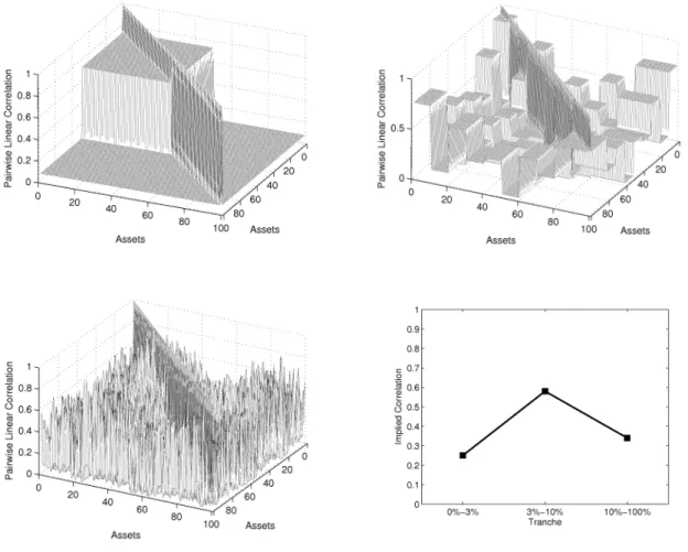
It is intuitively clear that different correlation structures can lead to identic tranche spreads and therefore to identic implied correlations. Consider first of all a flat corre-lation matrix A with uniform asset correcorre-lation 0.5. Using this correcorre-lation matrix we compute the CDO spreads for the equity, the mezzanine and the senior tranche. From these spreads we derive the implied correlations. Trivially we get the same implied correlation parameter of 0.5 for all three tranches. Obviously this example doesn’t lead to a correlation smile. However we had obtained the same tranche spreads and the same implied correlations if we would have used the following correlation matrix B: The matrix consists of five commensurate clusters of 20 assets. The intra sector correlations are (0.9754, 0.8994, 0.6069, 0.4700, 0.4281) the inter sector correlation is 0.3911 (cf. figure 1).
[Figure 1 about here]
In this special case the flat correlation matrix A and the clustered correlation matrix B produce identic tranche spreads. If we want to price a CDO whose underlying has the actual correlation structure B, we could alternatively use the standard market model with correlation parameter 0.5. It would lead to correct CDO margins. Unfortunately the last-mentioned example is an exception. Most realistic correlation matrices lead to correlation smiles. In general using the standard market model with only one single asset correlation leads to severe mispricing.
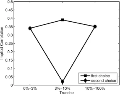
For instance, consider the following three dependence structures shown in figure 2. They all lead to identic tranche spreads and consequently to the same implied correla-tions (cf. figure 2). However the resulting tranche spreads can’t be replicated by using a flat correlation matrix, the standard market model would lead to mispricing.
[Figure 2 about here]
3.2
Heterogeneous Correlation Structures Can Cause Implied
Correlation Smiles
Note that the expected loss of the overall portfolio is independent of the default de-pendence structure of the assets in the portfolio. However the expected loss of single tranches depends on the correlation structure of the underlying. For instance when we modify a flat correlation matrix to a matrix with a cluster structure we change the risk of the tranches. Some tranches get riskier, some get less risky, some are more sensitive than others. To what extend the tranches react depends on their enhancement levels. Let’s consider a portfolio that consists of 10 separate commensurate clusters of high correlation amongst a background of low correlation (cf. figure 3). We observe that varying the difference between intra and inter cluster correlation influences the shape of the smile.
In the following figure 4 we examine the impact of keeping the intra sector correlation constant and varying the inter sector correlation. Keeping the inter sector correla-tion constant and varying the intra sector correlacorrela-tion results in correlacorrela-tion smiles too (cf. figure 5). The more the matrices differs from a flat correlation matrix the more pronounced is the smile.
[Figure 4 about here] [Figure 5 about here]
As mentioned above implied correlations for mezzanine tranches suffer from uniqueness problems. Sometimes two different implied correlation parameters can lead to identical spreads for mezzanine tranches. In the following examples we choose the correlation parameter that is closer to the implied correlation of the equity and the senior tranche (cf. figure 6).
[Figure 6 about here]
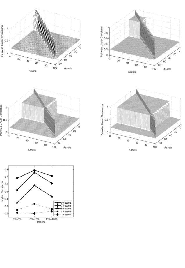
Now we consider a portfolio that is divided into separate sectors of equal size. We vary the size of these sectors and observe that an expanding cluster size influences the smile (cf. figure 7). If the underlying contains 4 clusters of 25 assets the observed smile is more intensive than the smile that is caused by 20 clusters of 5 assets. However the smile effect is only intensified up to a certain cluster size.
[Figure 7 about here]
Let’s finally consider a portfolio that contains only one single sector of high correlation. All other assets have low pairwise correlations (cf. figure 8). A negative correlation smile emerges depending on the cluster size. Again up to a certain cluster size the smile is aggravated by increasing the cluster size.
[Figure 8 about here]
4
Conclusion
In this paper we demonstrated that the explanatory power of implied correlations is rather questionable. We considered different dependence structures and examined the resulting correlation smiles. We chose a simplified Gaussian copula setup to make sure that the implied correlation smiles are solely due to the correlation matrix that descibes the dependence structure of the underlying. Our study suggests that the implied correlation smile that is observed in the market may be caused by an inhomo-geneous correlation structure of the actual underlying portfolio. Therefore we point out that relying on implied correlations may lead to severe mispricing of tranches. For the pricing of an off-market tranche that has the same underlying as a traded CDO we could take the implied correlation approach one step further and imply a depen-dence structure that reproduces all tranche spreads of the traded CDO simultaneously. Whenever it seems to be disproportionate to imply a full correlation matrix we can adjust the factor loadings of a one-factor approach or calibrate intra and inter sector correlations when the underlying assets belong to different highly correlated sectors. The implied dependence structure can then be used to compute the premium of the off-market tranche. We leave this idea for further research.
References
[1] Andersen, L. and Sidenius, J. (2004).Extensions to the Gaussian copula: random recovery and random factor loadings. The Journal of Credit Risk, 1(1): 29-70. [2] Andersen, L., Sidenius, J. and Basu, S. (2003).All your hedges in one basket. Risk,
November, pp. 67-72.
[3] Duffie, D. (2004).Time to adapt copula methods for modelling credit risk correla-tion. Risk, April, p. 77.
[4] Duffie, D. and Gbarleanu N. (2001). Risk and valuation of collateralized debt obli-gations. Financial Analysts Journal, 57(1): 41-59.
[5] Finger, C.C. (2004).Issues in the pricing of synthetic CDOs. The Journal of Credit Risk, 1(1): 113-124.
[6] Friend, A. and Rogge, E. (2004). Correlation at first sight. Forthcoming in Eco-nomic Notes: Review of Banking, Finance and Monetary EcoEco-nomics.
[7] Gregory, J. and Laurent, J.P. (2004).In the core of correlation. Risk, October, pp. 87-91.
[8] Hull, J. and White, A. (2004). Valuation of a CDO and an nth to default CDS
without Monte Carlo simulation. The Journal of Derivatives, 12(2): 8-23. [9] Jäckel, P. (2004). Splitting the core. Working Paper.
[10] Kamat, R. and Oks, M. (2004).Full correlation matrices for pricing credit portfolio tranches. Working Paper, FEA Research.
[11] Lando, D. (1998).On Cox processes and credit risky securities. Review of Deriva-tives Research, 2(2-3): 99-120.
[12] Laurent, J.P. and Gregory, J. (2003). Basket default swaps, CDOs and factor copulas. Forthcoming in The Journal of Risk.
[13] Li, D.X. (2000). On default correlation: a copula function approach. The Journal of Fixed Income, Vol. 9, March, pp. 43-54.
[14] Mashal, R., Naldi, M. and Tejwani, G. (2004). The implications of implied corre-lation. Lehman Brothers, Quantitative Credit Research Quarterly.
[15] McGinty, L., Beinstein, E., Ahluwalia, R. and Watts, M. (2004). Introducing base correlations. Working Paper, JPMorgan.
[16] Meneguzzo, D., Vecchiato, W. (2004). Copula sensitivity in collateralized debt obligations and basket default swaps. The Journal of Futures Markets, 24(1): 37-70.
[17] Mortensen, A. (2005). Semi-analytical valuation of basket credit derivatives in intensity-based models. Working Paper, Copenhagen Business School.
[18] Schönbucher, P.J. (2003). Credit derivatives pricing models: models, pricing and implementation. Wiley Finance Series, John Wiley & Sons, Chichester.
[19] Schönbucher, P.J. (2001).Copula-dependent default risk in intensity models. Work-ing Paper, University of Bonn.
[20] Tavares, P.A.C., Nguyen, T.U., Chapovsky, A., Vaysburd, I. (2004). Composite basket model. Working Paper, Merrill Lynch Credit Derivatives.
[21] Willemann, S. (2004). An evaluation of the base correlation framework for syn-thetic CDOs. Working Paper, Aarhus School of Business.
Figure 1: The flat correlation matrix A with correlation parameter 0.5 and the above-mentioned correlation matrix B with 5 clusters of 20 assets lead to identical implied correlations. This example doesn’t exhibit a smile.
Figure 2: We are able to construct correlation matrices that differ in shape but lead to identic tranche spreads and consequently to identic implied correlation parameters for the equity, the mezzanine and the senior tranche.
Figure 3: Keeping the intra sector correlation constant and varying the inter sector correlation influences the shape of the smile. Likewise we observe that the smile reacts to keeping the inter sector correlation constant and varying the intra sector correlation.
Figure 4: These implied correlation smiles are produced by a correlation matrix with 10 clusters of equal size. The intra sector correlation is 0.7, the inter sector correlation varies from 0.3 to 0.5.
Figure 5: These correlation smiles are produced by a correlation matrix with 10 clusters of equal size The inter sector correlation is 0.3, the intra sector correlation varies from 0.5 to 0.7.
Figure 6: The uniqueness problem. A correlation matrix with one cluster consisting of 25 assets with intra sector correlation 0.8 and inter sector correlation 0.3 leads to a mezzanine tranche spread that can be reproduced by two different flat correlation matrices.
Figure 7: The influence of a varying number of clusters on the correlation smile. We consider portfolios that consists of 2, 4, 10, 20 clusters. The intra sector correlation is 0.7, the inter sector correlation is 0.3.
Figure 8: The influence of the cluster size on the correlation smile when there is only one sector of high correlation. The size of the cluster varies between 10 and 90 assets, the intra sector correlation is 0.8, the inter sector correlation is 0.2.