The power of
-points in preemptive single
machine scheduling
Andreas S. Schulz
1;†and Martin Skutella
2;∗;‡1Massachusetts Institute of Technology;Sloan School of Management;E53-361;77 Massachusetts Avenue;
Cambridge MA 02139-4307;U.S.A.
2Technische Universitat Berlin;Institute fur Mathematik;MA 6-1;Strae des 17. Juni 136;
D-10623 Berlin;Germany
SUMMARY
We consider the NP-hard preemptive single-machine scheduling problem to minimize the total weighted completion time subject to release dates. A natural extension of Smith’s ratio rule is to preempt the currently active job whenever a new job arrives that has higher ratio of weight to processing time. We prove that the competitive ratio of this simple on-line algorithm is precisely 2. We also show that list scheduling in order of random -points drawn from the same schedule results in an on-line algorithm with competitive ratio 43. Since its analysis relies on a well-known integer programming relaxation of the scheduling problem, the relaxation has performance guarantee 43 as well. On the other hand, we show that it is at best an 8
7-relaxation. Copyright ? 2002 John Wiley & Sons, Ltd.
KEY WORDS: scheduling theory; approximation algorithm; on-line algorithm; randomized algorithm; LP relaxation; combinatorial optimization
1. INTRODUCTION
We study the preemptive single-machine on-line scheduling problem with release dates so as to minimize the average weighted completion time. A set of independent jobs J={1; : : : ; n} has to be scheduled on a single machine, where jobs arrive over time and the number of jobs is unknown in advance. Each job j∈J becomes available at its integral release date rj; which is not known in advance; at time rj we learn both its positive integral processing time pj and its non-negative weight wj. The machine cannot process more than one job at a time, and each job j has to be scheduled for pj time units on the machine. The processing of a job may repeatedly be interrupted and continued at a later point in time, i.e. we sequence in a preemptive fashion. For each time t; we must construct the schedule until time t without
∗Correspondence to: Martin Skutella, Technische Universitat Berlin, Fachbereich Mathematik, MA 6-1, Strae des 17. Juni 136, D-10623 Berlin, Germany
†E-mail: [email protected]
any knowledge of the jobs that will arrive afterwards. The aim is to minimize the sum of weighted job completion timesjwjCj or, equivalently, the average weighted completion time (1=n)jwjCj; here,Cj denotes the completion time of jobj in a schedule. The corresponding o-line optimization problem, where all job data is known in advance, is usually denoted by 1|rj; pmtn|wjCj [1]. It is strongly NP-hard [2].
The performance of an on-line algorithm is typically measured by its competitive ratio, which is the largest ratio of the objective function value achieved by the on-line algorithm to the value of the o-line optimum, taken over all instances. For randomized algorithms, we use expected objective function value in the denition of the competitive ratio. This corresponds to the so-called oblivious adversary model. We refer the reader to Reference [3] for a general introduction to on-line algorithms, and to Reference [4] for a survey of on-line scheduling. Because we will discuss at times the o-line scenario as well, let us introduce the related concept of an approximation algorithm. A -approximation algorithm is a polynomial-time algorithm that produces a solution of value not worse than times the optimal value. In case the algorithm has access to randomness, we call it a randomized -approximation algorithm, provided that it still runs in polynomial time; the performance guarantee , however, only needs to hold in expectation. Obviously, any on-line algorithm that runs in polynomial time and has competitive ratio is a -approximation algorithm.
The main result of this paper is a randomized on-line algorithm for 1|rj; pmtn|wjCj with competitive ratio 4
3 and running timeO(nlogn). For the o-line setting, it can be derandomized without loss of performance guarantee, but at the cost of an increased running time of O(n2). Our result also implies a bound of 4
3 on the quality of a well-known linear programming relaxation (which happens to be integer) of the problem under consideration. Moreover, we present a class of instances showing that the ratio between the true optimum and the LP lower bound can be arbitrarily close to 8
7.
The three key ingredients of the algorithm and its analysis are the conversion of a preemptive schedule to another preemptive schedule, the use of -points in connection with randomness to sample more information from the given preemptive schedule, and the ex-ploitation of a linear programming relaxation as a lower bound on the optimal objective function value. All three techniques have in recent years evolved as important tools to derive constant-factor approximation algorithms for a series of scheduling problems with min-sum objective.
The conversion of preemptive schedules to (non-preemptive) schedules was introduced by Phillipset al. [5] and was subsequently also used in References [6–8], among others. Slightly varying notions of -points were considered in References [5; 9], but their full potential was revealed when Chekuri et al. [7] as well as Goemans [8] chose the parameter at random. For 0¡61; the -point CjP() of job j with respect to a given (preemptive) schedule P is the rst point in time at which an -fraction of job j has been completed, i.e. when j has been processed on the machine for pj time units. In particular, CjP(1) =Cj and for= 0 we dene CjP(0) to be the starting time of job j. Later, -points with individual values of for dierent jobs have been used, see Reference [10]. We refer to Reference [11;Chapter 2] for a detailed account of approximation algorithms for min-sum criteria scheduling and -point scheduling.
The actual history of constant-factor approximation algorithms for 1|rj; pmtn|wjCj is rather short. Phillips et al. [5] designed an (8 + )-approximation algorithm for the more general problem of minimizing the average weighted completion time on unrelated parallel
machines subject to release dates. Hall et al. [12] gave a 2-approximation algorithm for the single-machine problem, in which there may also be precedence constraints among the jobs. Their algorithm is based on a related LP relaxation, rather than on the preemptive schedule that is an optimal solution of the integer programming relaxation that we employ in our analysis. In fact, it was Goemans [8] who rst showed that one can use this preemptive schedule to construct a non-preemptive schedule whose value is at most twice the optimal value of the integer programming relaxation. In particular, Goemans’ algorithm is a 2-approximation algorithm for 1|rj; pmtn|wjCj as well. Goemans et al. [13] then presented a randomized 1.466-approximation algorithm which also works in the on-line setting, as does the randomized variant of Goemans’ algorithm; our work may be seen as a simpler analysis of their algorithm that at the same time yields a better performance guarantee. Subsequently, a polynomial-time approximation scheme has been obtained for the o-line problem 1|rj; pmtn|wjCj; see Reference [14].
The rest of the paper is organized as follows. In Section 2 we embed the algorithm under consideration in the general class of preemptive list scheduling algorithms. Its actual analysis is given in Section 3. We conclude with some remarks on its derandomization and a discussion of open problems in Section 4.
2. PREEMPTIVE LIST SCHEDULING
There is a straightforward way to construct a feasible preemptive schedule from a given list of jobs representing some order: schedule at any point in time the rst available job in this list. Here, a job is available if its release time has elapsed. We refer to this routine as
preemptive list scheduling; the resulting schedule is calledpreemptive list schedule. Preemptive list scheduling has been used in various settings before, e.g. for minimizing the maximum lateness on a single machine [15]. An application of this routine in the context of min-sum criteria approximation has been proposed by Hall et al. [12] in order to turn an optimal solution to an LP relaxation in completion time variables into a feasible preemptive schedule. Goemans [8] showed that the routine can be used to construct an optimal solution to an LP relaxation in time-indexed variables; he also pointed out that preemptive list schedules can be constructed in O(nlogn) time using a priority queue.
As a consequence of the following lemma, one can in fact restrict to schedules that are generated by preemptive list scheduling.
Lemma 2.1
Given a feasible preemptive scheduleP, preemptive list scheduling in order of non-decreasing completion times does not increase completion times of jobs.
Proof
Although this lemma belongs to the folklore of the eld, let us provide a proof for the sake of completeness.
We denote the completion time of a jobjin the given schedule byCjP and in the preemptive list schedule by Cj. By construction, the new schedule is feasible since no job is processed before its release date. For a xed job j, let t¿0 be the earliest point in time such that there is no idle time in the preemptive list schedule during (t; Cj] and only jobs k with CkP6CjP
are processed. We denote the set of these jobs by K. By the denition of t, we know that
rk¿t, for all k∈K. Hence, CjP¿t+
k∈K pk. On the other hand, the denition ofK implies Cj=t+k∈K pk and therefore Cj6CjP.
An important property of preemptive list schedules is that whenever a job is preempted from the machine, it is only continued after all available jobs with higher priority are nished. Moreover, a job is only preempted if another job is released at that time. Therefore, since all release dates are integral, preemptions only occur at integral points in time. Throughout the paper we restrict to schedules meeting this property. Notice also that there are at most n−1 preemptions.
In the absence of non-trivial release dates there is no need for preemption and an optimal schedule can be constructed in O(nlogn) time using Smith’s ratio rule [16]: schedule the jobs in order of non-increasing ratios wj=pj. In the following, we will always assume that jobs are numbered such that w1=p1¿· · ·¿wn=pn; moreover, whenever we talk about scheduling in order of non-increasing ratios wj=pj, we refer to this order of jobs. A natural generalization of Smith’s Ratio Rule to 1|rj; pmtn|wjCj is preemptive list scheduling in order of non-increasing ratios wj=pj; notice that this algorithm also works on-line since at any point in time the ratios of all available jobs are known. Of course, the schedule constructed in this way is in general not optimal. The following lemma gives a lower bound on the performance of this simple heuristic.
Lemma 2.2
The competitive ratio of preemptive list scheduling in order of non-increasing ratios wj=pj is not better than 2, even if wj= 1 for all j∈J.
Proof
For an arbitrary n∈N, consider the following instance withnjobs. Let wj= 1; pj=n2−n+j; andrj=−n+j+kn=j+1pk, for 16j6n. Preemptive list scheduling in order of non-increasing ratios ofwj=pjpreempts jobjat timerj−1and nishes it only after all other jobsj−1; : : : ;1 have been completed. The value of this schedule is thereforen4−1
2n3+
1
2n. The shortest remaining processing time rule [17], which solves instances of 1|rj; pmtn|Cj optimally and does so on-line, sequences the jobs in order n; : : : ;1. It has value 1
2n
4+1
3n
3+1
6n. Consequently, the ratio of the objective function values of the ‘SPT-rule’ and the ‘SRPT-rule’ goes to 2 when
n goes to innity.
Notice that the negative result in Lemma 2.2 does not result from the on-line nature of the problem; it follows from the proof that this is rather an inherent drawback of preemptive list scheduling in order of non-increasing ratios wj=pj. On the other hand, one can give an upper bound of 2 on the performance of this algorithm. The following observation is due to Goemans, Wein and Williamson (personal communication, August 1997).
Lemma 2.3
Preemptive list scheduling in order of non-increasing ratios wj=pj has competitive ratio 2. Proof
We use two dierent lower bounds on the value Z∗ of an optimal solution in order to prove the claim. Since the completion time of a job is always at least as large as its release date, we
get Z∗¿jwjrj. The second lower bound is the value of an optimal solution for the relaxed problem in which all the release dates are zero. This yields Z∗¿j(wjk6jpk) by Smith’s ratio rule. Let Cj denote the completion time of job j in the preemptive list schedule. By construction one has Cj6rj+k6j pk and thus
j wjCj6 j wjrj+ j wj k6j pk 62Z∗
In spite of the negative result in Lemma 2.2, preemptive list scheduling in order of non-increasing ratios wj=pj can help to construct a preemptive schedule whose value is at most a factor 4
3 away from the optimum. The idea is to transform this schedule by preemptive list scheduling in order of non-decreasing -points. The underlying intuition is that the given schedule gives rise to dierent job orders if dierent values of are used. There is, however, no instance that is simultaneously bad for the preemptive list schedules obtained from all dierent values of. Consider for instance the example constructed in the proof of Lemma 2.2. For most values of ; the corresponding preemptive list schedule is optimal. We will analyse the following simple algorithm:
Algorithm 1
(1) Draw randomly from [0;1].
(2) Construct the preemptive list schedule P in order of non-increasing ratios wj=pj. (3) Apply preemptive list scheduling in order of non-decreasing CjP().
The on-line variant of Algorithm 1 constructs the two preemptive list schedules in Step 2 and Step 3 simultaneously. Notice that preemptive list scheduling can be implemented on-line if a job can be inserted at the correct position in the list with respect to the jobs that are already known, as soon as it becomes available. As already mentioned, preemptive list scheduling in order of non-increasing ratios wj=pj works on-line since at any point in time the ratios of all available jobs are known. Unfortunately, this is not true for the -points of jobs because the future development of the schedule in Step 2 is not known. However, at any point in time and for an arbitrary pair j; k of already available jobs we can predict whether
CP
j() will be smaller than CkP(), or not. If one or even both values are already known, we are done. Otherwise the job with higher priority in the ratio list of Step 2, say j, will win since job k cannot be (re)started in Step 2 before j is nished. Thus, we have proved that Algorithm 1 can be implemented as a randomized on-line algorithm. Since preemptive list scheduling runs in O(nlogn) time, the running time of Algorithm 1 and its on-line vari-ant is O(nlogn); too. For xed , we call the schedule computed in Step 3 preemptive -schedule.
Goemans analysed in Reference [8] a variant of Algorithm 1 in which the jobs are scheduled non-preemptively in order of non-decreasing -points, whereis chosen uniformly at random. Because the value of the resulting schedule is an upper bound on the value of the schedule computed in Step 3, it follows that Algorithm 1 has competitive ratio 2 in this case.
Goemans et al. [13] showed that Algorithm 1 achieves competitive ratio 1.466 if is chosen from the interval [0; ] according to a probability distribution with density function
The following theorem contains the main result of this paper.
Theorem 2.4
Let the random variablebe chosen from a probability distribution over [0,1] with the density function f() = 1 3(1−)− 2 if ∈[0; 1 2] 4 3 otherwise
Then, Algorithm 1 has competitive ratio 4 3.
The proof of Theorem 2.4 is presented in the next section. Besides the better performance ratio, its major advantage compared to the analysis in Reference [13] is its simplicity. In par-ticular, in contrast to Reference [13], our analysis is job-by-job, i.e. we compare the expected completion time of each job with its completion time in the integer programming relaxation.
3. ANALYSIS OF THE ALGORITHM
The analysis of Algorithm 1 is divided into three parts. First, we discuss an integer linear programming relaxation which gives a lower bound on the value of an optimal schedule. Then we derive a general upper bound on the completion time of an arbitrary job in the schedule computed by Algorithm 1, which depends on . Finally, in the third part, we compare the ex-pected value of this upper bound to the corresponding term in the integer linear programming relaxation derived in the rst part.
3.1. An integer linear programming relaxation
To obtain a good lower bound on the value of an optimal solution, we use an integer linear programming relaxation in time-indexed variables that was originally introduced by Dyer and Wolsey [18]. Although each integral feasible solution to this program corresponds to a feasible preemptive schedule, the program is a true relaxation of 1|rj; pmtn|wjCj since the objective function underestimates the value of a preemptive schedule. On the other hand, this integer linear program (ILP) can be solved to optimality in polynomial time such that we need not consider its LP relaxation.
The idea of the formulation is to discretize time between 0 and a xed horizon T+1 := maxjrj+jpj into intervals of length 1. One introduces binary variables yjt for each job j and each time interval (t; t+ 1]; t= 0;1; : : : ; T; where yjt= 1 if and only if job j is being processed during the time interval (t; t+ 1]. Note that T and thus the number of yjt-variables may be exponential in the input size of the scheduling problem. We get the following ILP:
minimize j∈J wjCjILP subject to T t=rj yjt=pj for all j∈J (1)
j∈Jyjt61 for t= 0; : : : ; T (2) CILP j = pj 2 + 1 pj T t=0 yjt(t+12) for all j∈J (3) yjt= 0 for all j∈Jand t= 0; : : : ; rj−1 (4) yjt∈ {0;1} for all j∈Jand t=rj; : : : ; T (5) Equations (1) ensure that the whole processing requirement of every job is satised. The machine capacity constraints (2) express that the machine can process at most one job at a time. Because of Equations (4), no job can be processed before its release date. The following lemma, due to Goemans [8], oers one way to understand Equations (3).
Lemma 3.1
Consider an arbitrary preemptive schedule P that is nished before time T + 1, and assign the values to the ILP variables yjt as dened above, i.e.yjt= 1 if j is being processed in the interval (t; t+ 1]; and yjt= 0 otherwise. Then,
1 0 CP j () d= 1 pj T t=0 yjt(t+ 12)6CjP− pj 2 (6)
for each job j, and equality holds if and only if job j is never preempted from the machine.
Proof
For a xed job j, denote by t; t= 0; : : : ; T + 1; the fraction of j that is nished in the preemptive schedule P by time t. Since 0 =0616· · ·6T+1= 1; we can write
1 0 CP j() d= T t=0 t+1 t CP j() d= T t=0 (t+1−t)(t+12) = T t=0 yjt pj(t+ 1 2)
which proves the equation in (6). Since CjP()6CjP−(1−)pj for 0661, we get 1 0 CP j () d6CjP−pj 1 0 (1−) d=CjP−pj 2
Equality holds if and only if CjP() =CjP −(1−)pj for all 0¡61, that is, i job j is scheduled non-preemptively.
As a consequence of Lemma 3.1, the value of an optimal solution to ILP is a lower bound on the value of an optimal preemptive schedule.
As pointed out by Dyer and Wolsey [18], it follows from the work of Posner [19] that ILP can be solved in O(nlogn) time. Goemans [8] showed that preemptive list scheduling in order of non-increasing ratios wj=pj denes an optimal solution to ILP if the variables yjt are set as described above. This basically follows from the observation that eliminating the variables CILP
j by plugging (3) into the objective function leads to a transportation problem, which can be solved in a greedy manner.
As a result, the encoding size of the optimal solution is polynomial in the input size and it can be constructed in time O(nlogn) although ILP itself may be exponentially large. In addition, Algorithm 1 computes an optimal solution to ILP in Step 2.
3.2. Preemptive -conversion
This subsection presents the insights into the structure of the preemptive list schedules com-puted in Step 2 and Step 3 of Algorithm 1 that are needed to prove Theorem 2.4.
For a xed jobj, we dene J to be the subset of J consisting of all jobs that are started beforejin the preemptive list scheduleP. Notice that no jobk∈J is being processed between the start and the completion time of j; ifk is not yet completed when j is started, then j¡k. We denote the fraction of job k∈J that is completed by time CjP(0) by k. Since we can write the starting time CjP(0) of job j as the amount of idle time plus the time during which the machine is busy processing jobs in J before j is started, we get
CP
j(0)¿
k∈Jkpk (7)
To analyse the completion times of jobs in the schedule computed in Step 3 of Algorithm 1 we consider schedules that are constructed by a slightly dierent o-line conversion routine, which we call preemptive -conversion.
Algorithm: Preemptive -conversion. Consider the jobs j∈J in order of non-increasing
CP
j() and iteratively change the current preemptive schedule by applying the following steps:
(i) postpone the whole processing that is done later than CjP() by (1−)pj;
(ii) remove the (1−)-fraction of job j that is being processed later than CjP() from the machine and shrink the corresponding time intervals;
(iii) process the removed fraction of job j in the released time interval (CjP(); CjP() + (1−)pj].
Note that the completion time of any job in the schedule produced by preemptive
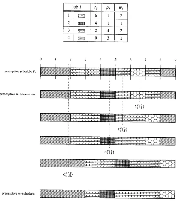
-conversion is not smaller than its completion time obtained from preemptive list scheduling according to non-decreasing CjP(); this follows from Lemma 2.1 since the order of comple-tion times in the preemptive -schedule coincides with the order of -points in P. Figure 1 depicts a small example with 4 jobs illustrating the action of preemptive -conversion.
Lemma 3.2
For xed , the completion time Cj of job j in the schedule computed by Algorithm 1 can be bounded by
Cj6CjP() + (1−)pj+
k∈J:k¿(1−k)pk (8) Proof
We prove that the right-hand side of (8) is equal to the completion time of job j in the schedule constructed by preemptive -conversion. Notice that preemptive -conversion does not modify the schedule P within the time interval [0; CjP()] before the iteration in which j is being converted. Therefore, directly after the conversion of job j its completion time in the current preemptive schedule is equal to CjP() + (1−)pj.
Figure 1. The conversion of the preemptive list schedule P by preemptive -conversion and by preemptive list scheduling in order of non-decreasing -points for =58.
Consider a subsequent iteration corresponding to a job k with CkP()¡CjP(). We distin-guish two cases: If CkP()¿CjP(0) then k¡j since job j is interrupted by k in the sched-ule P. In particular, k is completed before the processing of j is resumed in P. Therefore, the completion time of j in the current schedule is not aected by the total postponement in
Step (i) and the shrinking in Step (ii). If CkP()6CjP(0), then k∈J andk¿. In this case, Step (i) and Step (ii) cause a delay of the completion time of job j by (1−k)pk.
As already mentioned before, it follows from Lemma 2.1 that the completion time of job
j in the preemptive list schedule in order of non-decreasing -points is smaller than the completion time of job j in the schedule constructed by preemptive -conversion.
3.3. An appropriate probability distribution
The key to the analysis of Algorithm 1 is to bound the expected completion time of job
j in the resulting schedule by the expected value of the right-hand side of (8). We then compare the latter expected value to CILP
j in the optimal solution to ILP, which is computed in Step 2 of Algorithm 1. The following lemma highlights the connection between the chosen probability distribution and the achieved performance guarantee.
Lemma 3.3
Letf be a density function on [0;1] and denote the expected value of a random variable that is distributed according to f by Ef, i.e. Ef: =01f()d. Assume that¿0 and
(i) max∈[0;1]f()61 +, (ii) 1−Ef61+2,
(iii) (1−)0f() d6 for every ∈[0;1].
Moreover, let the random variablebe drawn from [0;1] according to a probability distribution with density functionf. Then, the expected completion time of every jobj∈J in the schedule constructed by Algorithm 1 is at most (1 +)CILP
j .
The intuition underlying the three conditions (i) – (iii) on the density functionfis to bound the expectations of the three corresponding terms on the right-hand side of (8) with respect to CILP j . Proof of Lemma 3.3 Lemma 3.2 yields E[Cj]6E[CjP()] +E[(1−)pj] +E k∈J:k¿(1−k)pk
The three terms on the right-hand side can be bounded as follows:
E[CjP()] =CjP(0) + 1 0 f()(CjP()−CjP(0)) d 6CP j(0) + (1 +) 1 0 (CjP()−CjP(0)) d by (i) = (1 +)CILP j −CjP(0)−(1 +) pj 2 by Lemma 3:1; E[(1−)pj] = (1−Ef)pj6(1 +)pj 2 by (ii);
E k∈J:k¿ (1−k)pk = k∈J(1−k)pk k 0 f() d 6 k∈J kpk6CjP(0) by (iii) and (7)
and the result follows. Notice that it is essential for the analysis to implicitly divide the interval [0; CjP()] into [0; CjP(0)] and (CjP(0); CjP()] in order to boundE[CjP()]. This division reects the structural insight that led to the introduction of the subset J.
Proof of Theorem 2.4
Observe that the density function f given in Theorem 2.4 meets the requirements (i) – (iii) of Lemma 3.3 for =1
3. Thus, the competitive ratio 4
3 follows from Lemma 3.3 by linearity of expectations.
Since inequalities (i) and (iii) are tight in the proof of Theorem 2.4, we can show that the density function f is optimal with respect to the analysis given in Lemma 3.3. Suppose that there exists a density function g that fulls properties (i) and (iii) for ¡1
3. Using (i), this leads to the following contradiction: Let =1
2, then (1−) 0 g() d=1 2− 1 2 1 1=2 g() d¿1 2− 1 2× 1 2× 4 3= 1 3 3.4. Further results
One can also prove a competitive ratio of 4
3 for the variant of Algorithm 1 where is chosen from the interval [0;3
4] according to the probability distribution with density function f() =13(1−)−2. Notice that this distribution is of the form as the one used in Reference [13] (with =3
4). However, the analysis is slightly more complicated in this case.
In our analysis of Algorithm 1 we have bounded the expected value of the computed schedule in terms of the lower bound given by an optimal solution to ILP. Thus, we have derived the same bound on the quality of the integer linear programming relaxation ILP.
Theorem 3.4
The relaxation ILP is a 43-relaxation, but it is not better than an 87-relaxation for the problem 1|rj; pmtn|wjCj.
Proof
The upper bound on the quality of ILP follows from the analysis of Algorithm 1. To prove the negative result, consider the following instance with n jobs, where n is assumed to be even. The processing times of the rst n−1 jobs j= 1; : : : ; n−1 are 1, their common release date is n=2, and all weights are 1=n2. The last job has processing timep
n=n, weightwn= 1=(2n), and is released at time 0. This instance is constructed such that every reasonable preemptive schedule without idle time on the machine has value 2−3=(2n). However, an optimal solution to ILP has value 7
4−5=(4n) such that the ratio goes to 8
4. CONCLUDING REMARKS
Goemans [8] observed that there are at most n combinatorially dierent values of , i.e. over all possible choices of one gets at most n dierent preemptive list schedules in order of
-points. Since each preemptive list schedule can be evaluated in O(n) time, this results in an o-line deterministic 43-approximation algorithm with running time O(n2) by choosing the best one from these schedules, i.e. the one with smallest weighted sum of completion times. We close by discussing some open questions that we regard as interesting. We have shown that ILP is a 4
3-relaxation of 1|rj; pmtn|
w
jCj and not better than an 87-relaxation. What is its true quality? Interestingly, the very same integer program is known to be a 1.686-relaxation for the non-preemptive problem 1|rj|wjCj. In this context, it is not better than a 1.581-relaxation. See Reference [10] for both results.
In the on-line setting, it seems that no good lower bound on the achievable competitive ratio of any on-line algorithm for the preemptive problem is known, neither for deterministic, nor for randomized algorithms. As for the upper bounds, we do not believe that the presented algorithms, which have competitive ratio 2 and 4
3, respectively, will be the ultimate answer. In contrast, the corresponding non-preemptive problem seems better understood. For the to-tal completion time objective (wj= 1 for all j∈J), Hoogeveen and Vestjens [20] as well as Phillips et al. [5] gave deterministic 2-competitive algorithms; Hoogeveen and Vestjens also showed that competitive ratio 2 is best possible for deterministic on-line algorithms. In Reference [7], Chekuri et al. presented a randomized e=(e−1)-competitive algorithm; Vestjens [21] proved this is optimal against oblivious adversaries. The best known determin-istic and randomized on-line algorithms for the more general total weighted completion time objective have competitive ratio 2.415 and 1.686, respectively, see References [8; 10]. They use ILP in the analysis and -points drawn from the corresponding preemptive schedule in the algorithm, as we do. The current knowledge on the cost of the lack of complete information is the same as in the unit-weight case.
Note added in Proof. The following new results were recently derived, which partly answer some of the open problems we had posed. Epstein and van Stee [23] gave lower bounds of 1.073 and 1.038 for the competitive ratio achievable by any deterministic respectively randomized on-line algorithm for 1|rj; pmtn|wjCj. Anderson and Potts [24] presented a deterministic 2-competitive algorithm for 1|rj|wjCj.
REFERENCES
1. Graham RL, Lawler EL, Lenstra JK, Rinnooy Kan AHG. Optimization and approximation in deterministic sequencing and scheduling: A survey.Annals of Discrete Mathematics1979;5:287–326.
2. Labetoulle J, Lawler EL, Lenstra JK, Rinnooy Kan AHG. Preemptive scheduling of uniform machines subject to release dates. InProgress in Combinatorial Optimization, Pulleyblank WR (ed.). Academic Press, New York, 1984; 245 –261.
3. Borodin A, El-Yaniv R. Online Computation and Competitive Analysis. Cambridge University Press: Cambridge, 1998.
4. Sgall J. On-line scheduling. In Online Algorithms:The state of the Art, Chapter 9, Fiat A, Woeginger GJ (eds). Springer, Berlin, 1998; 196 –231.
5. Phillips C, Stein C, Wein J. Minimizing average completion time in the presence of release dates.Mathematical ProgrammingB 1998; 82:199 –223
6. Chakrabarti S, Phillips C, Schulz AS, Shmoys DB, Stein C, Wein J. Improved scheduling algorithms for minsum criteria. InAutomata,Languages and Programming,Lecture Notes in Computer Science, vol. 1099, Meyer auf der Heide F, Monien B (eds). Springer: Berlin, 1996; 646 – 657.
7. Chekuri CS, Motwani R, Natarajan B, Stein C. Approximation techniques for average completion time scheduling. SIAM Journal on Computing, to appear. (An earlier version appeared in Proceedings of the 8th Annual ACM-SIAM Symposium on Discrete Algorithms, 1997; 609 –618).
8. Goemans MX. Improved approximation algorithms for scheduling with release dates. Proceedings of the 8th Annual ACM-SIAM Symposium on Discrete Algorithms 1997; 591– 598.
9. Hall LA, Shmoys DB, Wein J. Scheduling to minimize average completion time: O-line and on-line algorithms.
Proceedings of the 7th Annual ACM-SIAM Symposium on Discrete Algorithms1996; 142 – 151.
10. Goemans MX, Queyranne M, Schulz AS, Skutella M, Wang Y. Single machine scheduling with release dates, 1999. Submitted.
11. Skutella M. Approximation and randomization in scheduling. Ph.D. Thesis, Technische Universitat, Berlin, Germany, 1998.
12. Hall LA, Schulz AS, Shmoys DB, Wein J. Scheduling to minimize average completion time: O-line and on-line approximation algorithms.Mathematics of Operations Research1997;22:513 – 544.
13. Goemans MX, Wein JM, Williamson DP. A 1.47-approximation algorithm for a preemptive single-machine scheduling problem.Operations Research Letters2000;26:149 –154.
14. Afrati F, Bampis E, Chekuri C, Karger D, Kenyon C, Khanna S, Milis I, Queyranne M, Skutella M, Stein C, Sviridenko M. Approximation schemes for minimizing average weighted completion time with release dates. Proceedings of the 40th Annual IEEE Symposium on Foundations of Computer Science1999; 32–43. 15. Horn WA. Some simple scheduling algorithms.Naval Research and Logistics Quarterly1974;21:177–185. 16. Smith WE. Various optimizers for single-stage production. Naval Research and Logistics Quarterly 1956;
3:59 –66.
17. Baker KR.Introduction to Sequencing and Scheduling.Wiley: New York, 1974.
18. Dyer ME, Wolsey LA. Formulating the single machine sequencing problem with release dates as a mixed integer program. Discrete Applied Mathematics1990;26:255 –270.
19. Posner ME. A sequencing problem with release dates and clustered jobs. Management Science 1986;
32:731–738.
20. Hoogeveen JA, Vestjens APA. Optimal on-line algorithms for single-machine scheduling. In Integer Programming and Combinatorial Optimization, Lecture Notes in Computer Science, vol. 1084, Cunningham WH, McCormick ST, Queyranne M (eds). Springer: Berlin, 1996; 404–414.
21. Vestjens APA. On-line scheduling.Ph.D. Thesis, Eindhoven University of Technology, The Netherlands, 1997. 22. Goemans MX. A supermodular relaxation for scheduling with release dates. In Integer Programming and Combinatorial Optimization,Lecture Notes in Computer Science, vol. 1084, Cunningham WH, McCormick ST, Queyranne M (eds). Springer: Berlin, 1996; 288 –300.
23. Epstein L, van Stee R. Lower bounds for on-line single-machine scheduling. In Mathematical Foundations of Computer Science 2001, Lecture Notes in Computer Science, vol. 2136, Sgall J, Pultr A, Kolman (eds). Springer: Berlin, 2001; 338–350.
24. Anderson EJ, Potts CN. On-line scheduling of a single machine to minimize total weighted completion time.