Column subset selection for single-cell RNA-Seq
clustering
SHANNON R. MCCURDY∗, VASILIS NTRANOS, LIOR PACHTER
Summary
The first step in the analysis of single-cell RNA sequencing (scRNA-Seq) is dimensionality reduction, which reduces noise and simplifies data visualization. However, techniques such as principal components analysis (PCA) fail to preserve non-negativity and sparsity structures present in the original matrices, and the coordinates of projected cells are not easily interpretable. Commonly used thresholding methods avoid those pitfalls, but ignore collinearity and covariance in the original matrix. We show that a deterministic column subset selection (DCSS) method possesses many of the favorable properties of PCA and common thresholding methods, while avoiding pitfalls from both. We derive new spectral bounds for DCSS. We apply DCSS to two measures of gene expression from two scRNA-Seq experiments with different clustering workflows, and compare to three thresholding methods. In each case study, the clusters based on the small subset of the complete gene expression profile selected by DCSS are similar to clusters produced from the full set. The resulting clusters are informative for cell type.
∗To whom correspondence should be addressed.
c
Key words: Clustering; Column Subset Selection; Leverage scores; scRNA-Seq; Thresholding.
1. Introduction
Advances in RNA sequencing technology have recently made it possible to measure the genome-wide expression profile of single cells (Tanget al.,2009). This promising technology is not without computational and analytical challenges, some of which include quality control, quantification, normalization, technical variability, and other confounding factors such as batch effects (Stegle, Teichmann and Marioni,2015;Wagner, Regev and Yosef,2016). More general challenges stem from the high dimensionality of the expression profiles: for example, selecting informative features from within the expression profiles.
One use for single-cell RNA sequencing (scRNA-Seq) data is the characterization of hetero-geneity of expression within a population of cells and the discovery of new cell types through clustering of expression profiles (Zeisel et al.,2015). This note explores the following question: is it possible reduce the number of features in the expression profile without a large effect on the error rate for clustering and classification? This question is inspired by the quality control and technical variability challenges of scRNA-Seq. Common techniques for quality control and technical variability reduction include simple thresholding schemes and principal components analysis (PCA). Both of these techniques reduce the number of features in the data matrix.
One commonly used technique to reduce the number of features in the data matrix involves selecting columns from the original data matrixA, to form a column submatrixC, by thresholding the individual columns based on a score. Frequently used scores are on measures of abundance (Lun, McCarthy and Marioni,2016), empirical variance (Kwon, Fan and Kharchenko,2017), abundance and empirical variance (McCarthyet al.), and index of dispersion (empirical variance/mean) (Satija
et al.,2015;Trapnellet al.,2014). Read count thresholds are intended to reduce low-abundance
2013), as these genes are not considered informative. Variance thresholding methods assume that the most variable genes are responsible for the important differences between cells (McCarthyet al.). Index of dispersion thresholding has a natural interpretation in terms of formal hypothesis testing, when the null model for gene abundance is the Poisson distribution (Cox and Lewis, 1966). We call these methods simple thresholding methods, because the score for each columni depends only on columni. Furthermore, within each columni, covariance between the rows (cells) of that column is not taken into account. By selecting columns and not linear combinations of columns fromA, the elements ofC will maintain the properties of non-negativity, sparsity, and interpretability, an advantage over PCA, but there are no guarantees thatC will have similar properties to the original data matrixA.
Replacing the original data matrix of scRNA-Seq expression profiles with a rank-k PCA truncation of the profiles is another commonly used technique to reduce the number of features and the technical variability (Wagner, Regev and Yosef,2016). To understand the PCA truncation, we must establish some matrix notation that we will use throughout this note. We orient the original data matrix Aso that thenrows are cells anddcolumns are features, wheren < d. For PCA, singular value decomposition (SVD) is performed on the column-mean centered matrix
˜
A = A−1µT, where 1 is an n×1 column vector andµ = n1AT1is a d×1column vector of column-means. The sum of the spectrum of eigenvalues ofA ˜˜AT is proportional to the total empirical variance ofA. The rank-kPCA truncation ofA, which we callT˜, is the rank-k SVD truncation of A˜. SVD is reviewed in Sec. 6.1, and the formula for T˜ is provided there. As a consequence of the SVD, the spectrum of the square of the rank-kPCA truncationT˜ is identical to the spectrum of the square of the mean-centered data matrix A˜ up to rank k; PCA gives a rank-k approximation to the mean-centered data A˜ that preserves the maximum empirical variance ofA. PCA is performed to reduce technical variability under the assumption that the technical variation is primarily captured by the non-leading eigenvalues and eigenvectors ofA ˜˜AT.
The drawback of replacing the original data matrix with the rank-kPCA truncation of the data that it fails to preserve non-negativity and sparsity structures present in the original data matrix, and the coordinates of projected cells are not interpretable in terms of single features.
The goal of column subset selection (CSS) is to extract from a matrixAa column submatrixC
that conserves favorable properties, such as conditions on the spectrum of the column submatrix
C (Tropp, 2009). Like the simple thresholding methods, CSS maintains the properties of non-negativity, sparsity, and interpretability, and like PCA, CSS conserves favorable matrix properties. Similar to the simple thresholding methods discussed above, each column has a score, however in CSS algorithms, the score for each columni also depends on all of the other columns. We will consider rank-ksubspace leverage scores in this note. Leverage scores have been considered for regression diagnostics and outlier detection in statistics (Velleman and Welsch,1981;Chatterjee and Hadi, 1986) and were brought to prominence more recently in the context of randomized matrix algorithms (Drineas, Mahoney and Muthukrishnan,2006). The rank-ksubspace leverage score τi(Ak)for theithcolumn ofAis,
τi(Ak) =aTi (AkATk)
+a
i, (1.1)
where the ith column of A is an (n×1)-vector denoted by a
i, M+ denotes Moore-Penrose pseudoinverse of M, and Ak is the rank-k SVD approximation toA, defined in Sec. 6.1. The leverage scoreτi(Ak)can also be written as the solution to the following optimization problem (Cohenet al.,2015), τi(Ak) = min Akx=ai ||x||22 x∈R d, (1.2) where||x||2
2 refers to the Euclidean (L2) norm of the vectorx. The vectorxmeasures how easily the columnai can be written as a linear combination of the columns ofAk. Eqn.1.2shows that leverage scores capture the importance of each column ai in the column space ofAk and are sensitive to collinearity between columns. We illustrate this point with a toy example in Sec.2.1.
CSS algorithms select columns either with a random sampling procedure (such as inDrineas, Mahoney and Muthukrishnan(2006)) or a deterministic procedure. We showcase the deterministic CSS (DCSS) algorithm introduced byPapailiopoulos, Kyrillidis and Boutsidis(2014). Papailiopou-los, Kyrillidis and Boutsidis(2014) show that for datasets with power-law decay in τi(Ak), DCSS will select a least-squares approximation forA,CC†A, requiring fewer columns with the same accuracy than random sampling methods. One of the contributions of this note is a new bound for the spectrum of the square ofC selected by DCSS projected onto the rank-ksubspace that best approximatesA(Eqn.2.9). This bound means that, once bothC andAare projected onto the rank-k subspace that best approximatesA,CCT is “close" toAAT. Another consequence is that the Frobenius norm of C is bounded (Eqn.2.10). The Frobenius norm is a measure of the “size" of a matrix, so this bound provides confidence that the DCSS column matrixCis also similar in “size" toAandAk. In the event that DCSS is performed on a mean-centered matrixA˜, the Frobenius norm provides a measure of empirical variance. We also show a similar bound holds for random sampling (Eqn. 2.11), and under the assumption of power-law decay, DCSS requires fewer columns for the same error than random sampling.
In addition to the spectral bound, we present two case studies on two different scRNA-Seq experimental and analysis workflows to illustrate empirically the effect of thresholding features with DCSS compared to read count, variance, and index of dispersion on clustering and classification. To the best of our knowledge, this is the first time DCSS has been applied to scRNA-Seq data. The first case study is the genome-wide expression profiles of3,005cells from the mouse cortex and hippocampus (Zeiselet al.,2015) and the clustering workflow of Ntranoset al.(2016). The second case is the genome-wide expression profiles of4,423 cells from mouse bone marrow (Paul
et al.,2015) and the trajectory workflow ofSettyet al.(2016). In both case studies, DCSS reduces
the low abundance genes and maintains many of the most variable and over-dispersed genes. This shows that DCSS shares the best features of the simple thresholding methods and, like PCA, comes
with additional bounds on the spectrum. This supports our conclusion that DCSS can be used instead of the simple thresholding methods for quality control and to reduce technical variability, in addition to selecting informative features. In both case studies, only a small fraction of the features are necessary to obtain clusters reflecting cell types, consistent with results in (Kwon, Fan and Kharchenko, 2017). We show that the error rate between the clustering assignments computed with the complete expression profile and the reduced expression profile is small.
2. Methods
The aim of this note is to explore the effect of thresholding features, measurements of gene expression, with DCSS. We compare DCSS to simple thresholding methods and also to the complete data. These thresholding methods are the first step in the pre-processing workflow. In this section, we include the DCSS algorithm for completeness, and we describe the new bounds for DCSS.
2.1 The DCSS algorithm (Papailiopoulos, Kyrillidis and Boutsidis,2014)
Algorithm 1. The DCSS algorithm selects for the submatrix C all columns i with a rank-k subspace leverage score τi(Ak)above a threshold θ, determined by the error toleranceand the rank,k. The algorithm is as follows.
1. Choose the rank,k, and the error tolerance, .
2. For every columni, calculate the rank-k subspace leverage scoresτi(Ak)(Eqn.1.1). 3. Sort the columns byτi(Ak), from largest to smallest. The sorted column indices areπi.
4. Define an empty set Θ = {}. Starting with the largest sorted column index π0, add the
corresponding column index ito the setΘ, in decreasing order, until,
X
i∈Θ
and then stop. Note thatk=Pd
i=1τi(Ak). It will be useful to define ˜=Pi6∈Θτi(Ak). Eqn. 2.3can equivalently be written as >˜.
5. . If the set size|Θ|< k, continue adding columns in decreasing order until|Θ|=k.
6. The leverage score τi(Ak) of the last column i included in Θ defines the leverage score threshold θ.
7. Introduce a rectangular selection matrixSof size d× |Θ|. If the column indexed by(i, πi)is inΘ, thenSi,πi = 1.Si,πi = 0otherwise. The DCSS submatrix is C=AS.
Theorem 3 ofPapailiopoulos, Kyrillidis and Boutsidis (2014) states that when the rank-k subspace leverage scores exhibit a power-law decay in the sorted column indexπi,
τπi(Ak) =π
−a
i τπ0(Ak) a >1, (2.4)
the number of sample columns selected by DCSS is,
|Θ|= max 2k 1a−1, 2k (a−1) a−11 −1, k . (2.5)
Papailiopoulos, Kyrillidis and Boutsidis(2014) demonstrate the power-law decay behavior of many real-world datasets; we show that this behavior is a reasonable assumption for the scRNA-Seq applications in Sec.3.
For a statistical interpretation of DCSS, consider the data ai, i = 1, . . . , d to be identi-cally and independently distributed (i.i.d.) according to the degenerate multivariate distribution N(0,AkATk). SeeRao(1973) pg. 527-528 for a discussion of the degenerate multivariate distribu-tion. Then the total likelihood of the data matrixAis,
L(A) = 1 (2π)12kdQk j=1|σj|d exp −1 2 d X i=1 aTi AkATk + ai ! = 1 (2π)12kdQk i=j|σj|d exp −1 2 d X i=1 τi(Ak) ! , (2.6)
where|σj|are thek largest singular values ofAk. In contrast, the total likelihood of the DCSS matrixCis, L(C) = 1 (2π)12k|Θ|Qk j=1|σj||Θ| exp −1 2 X i∈Θ τi(Ak) ! = 1 (2π)12k|Θ|Qk j=1|σj||Θ| exp − 1 2 X i∈Θ τi(Ak)−12 X i6∈Θ τi(Ak) +12˜ =L(A) exp 12˜ (2π)12k(d−|Θ|) k Y j=1 |σj|d−|Θ|. (2.7)
This shows that the DCSS matrixC preserves the total likelihood of the data up to a factor of
exp 12˜
<exp 12
and a normalization constant, under the assumption that the data is i.i.d. according toN(0,AkATk). Any other selection setΘ0 of the same number of columns (|Θ0|=|Θ|) will have equal or greater error ( 6 0). This interpretation illustrates that DCSS accounts for covarianceAkATk between rows (cells). In contrast, the Poisson null model for the index of dispersion assumes independence between rows (cells) for each column (gene).
The DCSS method has two parameters,k, which jointly determine the number of columns |Θ|in the DCSS column submatrix C. The parameterk determines the rank of interest of the SVD approximation to A. The tuning parameter is a measure of the error tolerance in the “size" ofC compared toAk. The selection of these parameters is a model selection problem, and in concert with a loss function, one could select these parameters using one’s preferred model selection method (e.g. cross-validation). The aim of this note, to compare clustering performed with the complete data matrix and a column submatrix, does not have a well-defined loss function, and so we use the heuristic “elbow" method for selectingk(Jolliffe,2002), and we chooseto be
0.1or0.05in our applications.
As a toy example to illustrate how DCSS differs from the simple thresholding methods, consider the following toy data matrix,
A= 40 20 10 20 10 15 . (2.8)
If the goal is to select a column submatrix with two columns, it is easy to check that simple thresholding by mean, variance, and index of dispersion all select the first and second columns. However, the resulting column submatrix is only rank1, because the first and second columns are linearly dependent. In contrast, DCSS with(k= 2, >0.2)will select the first and third columns, and the resulting DCSS column submatrix will be rank 2. Unlike the first three methods, DCSS takes into account the collinearity between columns in the selection procedure. If the DCSS error tolerance for this toy example is less than0.2, DCSS will select all three columns.
We also mention two asides: first, in applications where the number of cells is far greater than the number of gene features (n > d), the method can instead be applied toAT instead ofAto filter cells instead gene features; second, the method can be modified to select columns for any rank-ksubspace defined byksingular vectors ofA, and not just the leading-ksubspace (e.g. drop component1but include component2). This could be useful when some of the leading singular vectors are highly correlated with batch or other confounding effects.
2.2 New bounds for DCSS
We derive a new spectral approximation bound (Bound2.9) for the square of the submatrixC
selected with DCSS and projected onto the rank-ksubspace that best approximatesA.
Theorem2.1 LetA∈Rn×d be a matrix of at least rankkandτi(Ak)be defined as in Eqn.1.1. ConstructCfollowing the DCSS algorithm described in Sec.2.1. ThenCsatisfies,
(1−)AkATk UkUTkCC T
UkUTk AkATk. (2.9)
The symboldenotes the Loewner partial ordering which is reviewed in Sec6.1. Conceptually, the Loewner ordering is the generalization of the ordering of real numbers (e.g.1<1.5) to Hermitian matrices. This bound means that after projection onto the rank-ksubspace that best approximates
important consequences include inequalities for the eigenvalues and Euclidean distances. Some of the consequences of the Loewner ordering are reviewed in Sec6.1. Bound2.9and the fact that
CCT AAT implies a bound on the Frobenius norm ofC, a measure of the “size" of a matrix,
(1−)||Ak||2F 6||C|| 2
F 6||A|| 2
F. (2.10)
In the event thatAis mean-centered, this means that the total empirical variance ofCis bounded from below by(1−)the variance inAk and bounded from above by the total variance ofA. The proof of Bound2.9and Bound2.10is included in Sec.6.2.
One simple consequence of Bound2.9is the following bound,
(1−)AkATk UkUTkCC TU
kUTk (1 +)AkATk. (2.11)
Bound2.11also holds forCselected by random sampling methods withtcolumns (see Sec. 6.3for the theorem and proof). Thus, DCSS selects fewer columns with the same accuracyin Bound2.11for power-law decay in the rank-ksubspace leverage scores when,
|Θ|= max 2k 1a −1, 2k (a−1) a−11 −1, k < 22(k+mγ) 1 + 1 3 ln 16kδ 6t. (2.12)
In this expression,mis the number of columns with zero rank-ksubspace leverage score,γis the minimum non-zero leverage score, andδ is the probability that Bound2.11 fails to hold under random sampling.
3. Results
We present two case studies where we compare DCSS to the simple thresholding methods of variance, count, and index of dispersion. We analyze the overlap in the selected columns. We also illustrate the effect of DCSS compared to the complete data for single-cell clustering.
3.1 Zeisel et al.(2015)
As a concrete illustration of the DCSS method, we focus on the genome-wide expression profiles of 3005cells from the mouse somatosensory cortex and hippocampal CA1 region (Zeisel et al., 2015) and the clustering workflow ofNtranoset al.(2016). The main contribution ofNtranoset al.(2016) is to perform clustering directly on the partition of reads into equivalence classes (ECs) rather than on a full quantification of reads into gene expression. ECs are a partition of reads into distinct classes, such that every read in a class maps to exactly the same set of transcripts (Nicolaeet al.,2011). This method is computationally scalable, comparable across scRNA-Seq experiments, and can be more accurate than clustering performed on a full quantification of reads into gene expression profiles (Ntranoset al.,2016).
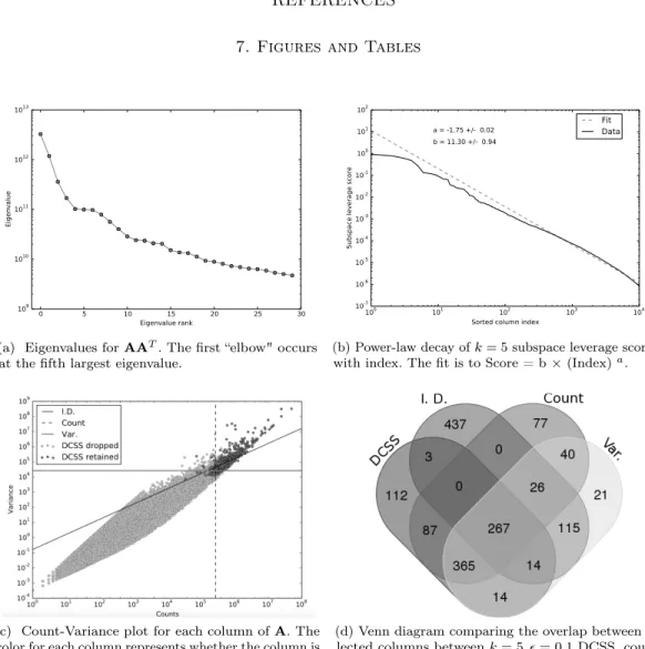
TheNtranoset al.(2016) data matrixAis3,005cells×246,981EC counts. By the elbow method, we choosek= 5for the DCSS workflow (Fig. 1a). We select an error tolerance of= 0.1. The rank-5subspace leverage scores and the power-law fit for the top-scored 10,000ECs are shown in Fig.1b. The column submatrixC has only862ECs, or approximately0.3%of the total ECs. These ECs contain 42.3% of the reads. These862 ECs map to2,748transcripts and to
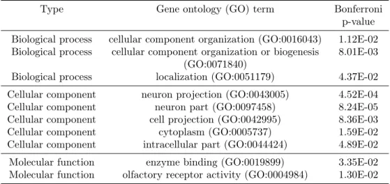
1,642genes. Table1contains the gene ontology term enrichment analysis (The Gene Ontology Consortium,2015) on the genes corresponding to the DCSS(k= 5, = 0.1)ECs. Enrichments relevant for the brain include neuron part, neuron projection, and olfactory receptor activity. The enrichment analysis has an important caveat: because we map ECs to transcripts without positing an error model, there could be a high rate of false positives in the resulting transcripts and genes. We compare DCSS to the three simple thresholding methods with the same number of columns in Fig. 1c and Fig. 1d. These figures show the similarities and differences in columns selected by the four thresholding methods. The simple thresholding methods have sharp boundaries in Fig. 1c, while the DCSS boundary is not linearly separable. The DCSS boundary approximately interpolates between the count and variance boundaries, and is most distinct from the index of
dispersion boundary. Fig.1dsummarizes the overlap between selected columns in a Venn diagram. These figures illustrate that the DCSS method selects columns that are highly variable, have large counts, and frequently are over-dispersed; as such, the DCSS method is prescribed for quality control and to control technical variability.
TheNtranoset al. (2016) workflow for theZeiselet al.(2015) dataset is to perform spectral clustering on pairwise Jensen-Shannon (JS) distances derived from the partition of reads into ECs. The spectral clustering clustering algorithm used is standard; the algorithm is to performk-means clustering on thek-dimensional SVD projection of the normalized Laplacian of the symmetric similarity matrixS. The similarity matrix used for spectral clustering isS(p,q) = 1−DJ S(p,q), whereDJ S(p,q)is the JS distance between two probability mass functionsp,q∈Rd. JS distances are well-suited to high-dimensional data, and provide more accurate clustering than L2distances on scRNA-Seq data (Ntranos et al., 2016). For the Zeisel et al. (2015) data, the probability mass function for each cell is the vector of EC counts, normalized to sum to one. For the four thresholded workflows (DCSS, count, variance, and index of dispersion), the probability mass function for each cell is the subset vector of EC counts, normalized to one.
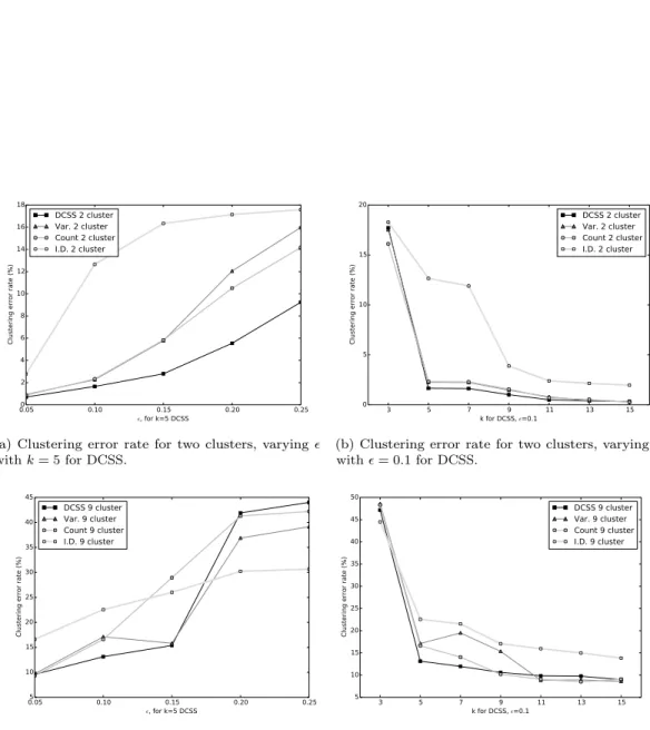
We evaluate the average spectral clustering classification error between the complete data and thresholded workflows, regarding the complete data workflow as the ground-truth. Since spectral clustering requires a random initialization fork-means, the average is overT = 10random initializations. Fig.2shows the average spectral clustering classification error rate for both two and nine spectral clusters for the workflow with the matrix Aand the workflow with the column submatrix C for variousk, . The different cells were curated into 47 subtypes byZeisel et al. (2015), but we evaluate our method on courser-grained classifications because we have higher confidence in the spectral clustering ground-truth. Two spectral clusters identify neurons and non-neurons, while nine spectral clusters only loosely correspond to the nine major cell types. We also include the error for the three simple thresholding methods with the same number of columns
as the DCSS method. We find that0.3%of the total ECs give an error rate of1.7%compared to the complete data for two clusters for k= 5, = 0.1DCSS; only a small fraction of the gene expression profiles currently produced in scRNA-Seq experiments may be necessary to obtain the clusters reflecting cell types.
3.2 Paul et al. (2015)
As a second application of the DCSS method, we focus on the genome-wide mRNA expression profiles of 4,423 cells from mouse bone marrow myeloid progenitors (Paul et al., 2015), and thewishbone trajectory workflow ofSettyet al.(2016). The contribution of Settyet al.(2016) to scRNA-Seq is to use diffusion maps to identify components related to the development and maturation of cells, specifically myeloid and erythroid progenitors from hematopoietic stem and progenitor cells (HSPCs).
The Settyet al. (2016) data matrix for the (Paul et al., 2015) dataset is A is 4,423 cells × 14,955gene unique molecular identifier (UMI) counts. The Setty et al. (2016) workflow is quite involved. In brief, the wishbone algorithm creates a nearest-neighbor Euclidean distance graph. This graph is used to estimate all of the shortest path distances between a set of randomly sampled cells and the rest of the cells, and the shortest path distances are used to make the trajectory and branch assignments. Thewishbone algorithm acts on a set of diffusion components which are selected for immune cell differentiation through a gene-set enrichment analysis. The diffusion components are calculated from the diffusion map of the similarity matrix derived from the Gaussian kernel of the10-nearest-neighbor Euclidean distance matrix from the15-dimensional PCA projection of the normalized UMI gene counts (Settyet al.,2016).
We choosek= 14for the DCSS workflow by the elbow method (Fig.3a). We choosek= 14
rather than an elbow at a smallerkbecause the diffusion component workflow is sensitive to more components. We select an error tolerance of = 0.05. The rank-14subspace leverage scores and
the power-law fit for the top-scored5,000genes are shown in Fig.3b. The column submatrixC
has4,693genes, or approximately31.4%of the total genes. These genes contain90.4% of the UMI counts.
We compare DCSS thresholding withk= 14, = 0.05to the three simple thresholding methods with the same number of columns in Fig.3c and Fig. 3d. The distribution of columns on the count-variance plots are qualitatively different between thePaulet al.(2015) data (Fig.3c) and the (Zeisel et al.,2015) data (Fig.1c). This difference is expected due to the differences between ECs and gene UMI counts. Although the index of dispersion method is more differentiated from the other methods on thePaulet al. (2015) dataset, the behavior of the DCSS method in relation to the simple thresholding methods is similar between the datasets.
We calculate the average wishbone classification error between the two workflows, again regarding the complete data workflow as the ground-truth. Since thewishbone algorithm utilizes random sampling, the average is overT = 10wishbone branch assignments. The originalwishbone analysis included only diffusion components1and2. We additionally include diffusion component
4, since it is also enriched for immune cell differentiation according to the GSEA. For thePaulet al.(2015) dataset,wishbone assigns cells to three branches. Settyet al.(2016) used the behavior of four markers (CD34, Gata1, Gata2, and Mpo) to verify that the three branches correspond to HSPCs, myeloid progenitors, and erythroid progenitors, and the behavior does not change with the inclusion of component4. Fig.3 shows the average branch assignment classification error rate for the workflow with the matrixAand the workflow with the column submatrixCfor variousk, , and also the three simple thresholding methods with the same number of columns as the DCSS method for eachk, point. Not all the thresholding methods successfully complete thewishbone workflow at large, due to the sensitivity of the diffusion component GSEA enrichment analysis, which we perform with keyword string matching. We find that for thek= 14, = 0.05 DCSS,
complete data; this supports our conclusion that only a small fraction of the gene expression profile from scRNA-Seq experiments may be necessary to obtain meaningful cell-type classifications.
4. Discussion
scRNA-Seq experiments allow researchers to probe the cell-specific heterogeniety in gene expression. Quality control and technical variability are significant challenges for scRNA-Seq experiments, and additionally the whole-genome expression profile is high-dimensional. In this note, we explore three existing simple thresholding schemes– count, variance, and index of dispersion– and propose a novel application of a thresholding scheme – DCSS– to select informative features and control quality and technical variability. We prove a bound on the “closeness" of the DCSS data submatrix to the complete data matrix (Eqn.2.9), enlarging upon the existing set of error guarantees for DCSS (Papailiopoulos, Kyrillidis and Boutsidis,2014), and illustrating the advantage of DCSS over the three simple thresholding schemes. Other advantages of DCSS include sensitivity to collinearity of features and covariance of cells. Since scRNA-Seq experiments are frequently used to cluster and classify cells, we choose the error rate for clustering and classification compared to the complete data as the evaluation metric for these thresholding schemes.
We present two case studies, the first on mouse cortex and hippocampus scRNA-Seq (Zeisel
et al.,2015;Ntranoset al.,2016), and the second on mouse bone marrow scRNA-Seq (Paul et
al.,2015;Settyet al.,2016). For the mouse cortex, the data matrix is cells×ECs, and only an incredibly small fraction of the ECs are necessary to obtain neuron and non-neuron cell clusters. For the mouse bone marrow, the data matrix is cells×genes, and only a small fraction of the genes are necessary to obtain HSPC, myeloid progenitor, and erythroid progenitor branch assignments. For both case studies, DCSS performs similarly to the simple thresholding schemes, in that it reduces the low abundance genes, maintains the most variable and over-dispersed genes. This supports our recommendation to use DCSS to control quality and technical variability. In both
case studies, the error rate between the clustering computed with the complete expression profile and the reduced expression profile is small, suggesting that the clustering algorithms rely on a small subset of informative features.
5. Software
The Python-package containing code to perform the methods described in the article can be found athttps://github.com/srmcc/dcss_single_cell.git. The package also contains code to download the datasets used as examples in the article.
Acknowledgments
Research reported in this publication was supported by the National Human Genome Research Institute of the National Institutes of Health under Award Number [F32HG008713]. The content is solely the responsibility of the authors and does not necessarily represent the official views of the National Institutes of Health. SRM would like to acknowledge Ilan Shomorony and Robert Tunney for useful comments.
Conflict of Interest: None declared.
References
Bourgon, Richard, Gentleman, Robert and Huber, Wolfgang. (2010, May). Independent filtering increases detection power for high-throughput experiments. Proceedings of the National
Academy of Sciences of the United States of America 107(21), 9546–9551.
Brennecke, Philip, Anders, Simon, Kim, Jong Kyoung, Kołodziejczyk, Aleksandra A., Zhang, Xiuwei, Proserpio, Valentina, Baying, Bianka, Benes, Vladimir, Teichmann, Sarah A., Marioni, John C.et al. (2013, November). Accounting for technical noise in
single-cell RNA-seq experiments. Nature Methods 10(11), 1093–1095.
Chatterjee, Samprit and Hadi, Ali S. (1986, August). Influential Observations, High
Leverage Points, and Outliers in Linear Regression. Statistical Science 1(3), 379–393.
Cohen, Michael B., Lee, Yin Tat, Musco, Cameron, Musco, Christopher, Peng, Richard and Sidford, Aaron. (2015). Uniform Sampling for Matrix Approximation. In:
Proceedings of the 2015 Conference on Innovations in Theoretical Computer Science, ITCS ’15. New York, NY, USA: ACM. pp. 181–190.
Cohen, Michael B., Musco, Cameron and Musco, Christopher. (2017). Input Sparsity
Time Low-rank Approximation via Ridge Leverage Score Sampling. In: Proceedings of the Twenty-Eighth Annual ACM-SIAM Symposium on Discrete Algorithms, SODA ’17. Philadelphia,
PA, USA: Society for Industrial and Applied Mathematics. pp. 1758–1777.
Cox, D. R. and Lewis, P. A. W.(1966). The statistical analysis of series of events, Methuen’s
monographs on applied probability and statistics. London: Methuen.
Drineas, Petros, Mahoney, Michael W. and Muthukrishnan, S. (2006). Subspace
sampling and relative-error matrix approximation: Column-based methods. In:In Proc. of the
10th RANDOM. pp. 316–326.
Eckart, C. and Young, G.(1936). The approximation of one matrix by another of lower rank.
Psychometrika 1, 211–218.
Horn, Roger A. and Johnson, Charles R. (2013). Matrix analysis, 2nd ed edition. New
York: Cambridge University Press.
Jolliffe, I. T.(2002). Principal component analysis, 2nd ed edition., Springer series in statistics.
Kwon, Haejoon, Fan, Jean and Kharchenko, Peter. (2017, January). Comparison of
Principal Component Analysis and t-Stochastic Neighbor Embedding with Distance Metric Modifications for Single-cell RNA-sequencing Data Analysis. bioRxiv, 102780.
Lun, Aaron T. L., McCarthy, Davis J. and Marioni, John C. (2016). A step-by-step
workflow for low-level analysis of single-cell RNA-seq data with Bioconductor. F1000Research 5, 2122.
McCarthy, Davis J., Campbell, Kieran R., Lun, Aaron T. L. and Wills, Quin F.
Scater: pre-processing, quality control, normalization and visualization of single-cell RNA-seq data in R. Bioinformatics.
Nicolae, Marius, Mangul, Serghei, Măndoiu, Ion I. and Zelikovsky, Alex. (2011).
Estimation of alternative splicing isoform frequencies from RNA-Seq data. Algorithms for molecular biology: AMB 6(1), 9.
Ntranos, Vasilis, Kamath, Govinda M., Zhang, Jesse M., Pachter, Lior and Tse, David N.(2016). Fast and accurate single-cell RNA-seq analysis by clustering of transcript-compatibility counts. Genome Biology 17(1), 1–14.
Papailiopoulos, Dimitris, Kyrillidis, Anastasios and Boutsidis, Christos. (2014).
Provable Deterministic Leverage Score Sampling. In:Proceedings of the 20th ACM SIGKDD
International Conference on Knowledge Discovery and Data Mining, KDD ’14. New York, NY,
USA: ACM. pp. 997–1006.
Paul, Franziska, Arkin, Ya’ara, Giladi, Amir, Jaitin, Diego Adhemar, Kenigs-berg, Ephraim, Keren-Shaul, Hadas, Winter, Deborah, Lara-Astiaso, David, Gury, Meital, Weiner, Assaf, David, Eyal, Cohen, Nadav, Lauridsen, Felicia Kathrine Bratt, Haas, Simon, Schlitzer, Andreas, Mildner, Alexander, Ginhoux,
Florent, Jung, Steffen, Trumpp, Andreas, Porse, Bo Torben, Tanay, Amos et
al. (2015, December). Transcriptional Heterogeneity and Lineage Commitment in Myeloid Progenitors. Cell 163(7), 1663–1677.
Rao, C. Radhakrishna. (1973). Linear statistical inference and its applications, 2d ed edition., Wiley series in probability and mathematical statistics. New York: Wiley.
Satija, Rahul, Farrell, Jeffrey A., Gennert, David, Schier, Alexander F. and Regev, Aviv. (2015, May). Spatial reconstruction of single-cell gene expression data. Nature Biotechnology 33(5), 495–502.
Setty, Manu, Tadmor, Michelle D., Reich-Zeliger, Shlomit, Angel, Omer, Salame, Tomer Meir, Kathail, Pooja, Choi, Kristy, Bendall, Sean, Friedman, Nir and Pe’er, Dana. (2016, June). Wishbone identifies bifurcating developmental trajectories from
single-cell data. Nature Biotechnology 34(6), 637–645.
Stegle, Oliver, Teichmann, Sarah A. and Marioni, John C.(2015, March). Computational
and analytical challenges in single-cell transcriptomics.Nature Reviews. Genetics16(3), 133–145.
Tang, Fuchou, Barbacioru, Catalin, Wang, Yangzhou, Nordman, Ellen, Lee, Clarence, Xu, Nanlan, Wang, Xiaohui, Bodeau, John, Tuch, Brian B., Siddiqui, Asim, Lao, Kaiqinet al.(2009, May). mRNA-Seq whole-transcriptome analysis of a single
cell. Nature Methods 6(5), 377–382.
The Gene Ontology Consortium. (2015, January). Gene Ontology Consortium: going forward.
Nucleic Acids Research 43(D1), D1049–D1056.
Trapnell, Cole, Cacchiarelli, Davide, Grimsby, Jonna, Pokharel, Prapti, Li, Shuqiang, Morse, Michael, Lennon, Niall J., Livak, Kenneth J., Mikkelsen,
Tar-jei S. and Rinn, John L.(2014, April). The dynamics and regulators of cell fate decisions
are revealed by pseudotemporal ordering of single cells. Nature Biotechnology 32(4), 381–386.
Tropp, Joel A.(2009). Column Subset Selection, Matrix Factorization, and Eigenvalue
Op-timization. In: Proceedings of the Twentieth Annual ACM-SIAM Symposium on Discrete
Algorithms, SODA ’09. Philadelphia, PA, USA: Society for Industrial and Applied Mathematics.
pp. 978–986.
Tropp, Joel A.(2015, May). An Introduction to Matrix Concentration Inequalities. Found.
Trends Mach. Learn.8(1-2), 1–230.
Velleman, Paul F. and Welsch, Roy E.(1981). Efficient Computing of Regression Diagnostics.
The American Statistician 35(4), 234–242.
VIB / UGent Bioinformatics and Evolutionary Genomics. Calculate and draw custom Venn diagrams: http://bioinformatics.psb.ugent.be/webtools/Venn/.
Wagner, Allon, Regev, Aviv and Yosef, Nir. (2016, November). Revealing the vectors of
cellular identity with single-cell genomics. Nature Biotechnology34(11), 1145–1160.
Zeisel, Amit, Muñoz-Manchado, Ana B., Codeluppi, Simone, Lönnerberg, Peter, Manno, Gioele La, Juréus, Anna, Marques, Sueli, Munguba, Hermany, He, Liqun, Betsholtz, Christer, Rolny, Charlotte, Castelo-Branco, Gonçalo, Hjerling-Leffler, Jenset al. (2015, March). Cell types in the mouse cortex and hippocampus revealed
6. Appendix
6.1 Brief linear algebra review (Horn and Johnson,2013)
Thesingular value decomposition (SVD) of any complex matrixAisA=UΣV†, where Uand
Vare square unitary matrices (U†U=UU† =I,V†V=VV† =I),Σis a rectangular diagonal matrix with real non-negative non-increasingly ordered entries.U† is the complex conjugate and transpose ofU, andIis the identity matrix. The diagonal elements ofΣ are called thesingular
values, and they are the positive square roots of the eigenvalues of bothAA† andA†A, which
have eigenvectorsUandV, respectively.UandV are theleft andright singular vectors ofA. DefiningUk as the firstkcolumns of Uand analogously for V, andΣk the square diagonal matrix with the firstkentries ofΣ, thenAk=UkΣkVk† is the rank-kSVD approximation toA, andT=AVk=UkΣk is a rank-kSVD truncation ofA. Furthermore, we refer to matrix with only the lastn−kcolumns of U,Vand lastn−k entries inΣas U\k,V\k, and Σ\k.
The Moore-Penrose pseudo inverse of a rankrmatrixAis given byA+=U
rΣ−r1Vr†. The Frobenius norm||A||F of a matrixAis given by||A||F =
p
tr(AA†). The spectral norm ||A||2of a matrix Ais given by the largest singular value ofA.
The Eckart-Young-Mirsky theorem (Eckart and Young,1936) states that, for A=UΣV† the SVD ofA, andB any complex matrix with compatible dimension toAand rank6k,
Ak=argminrank(B)6k||A−B||F min rank(B)6k ||A−B||F = q tr(Σ\kΣT\k). (6.13)
The minimizerAk is unique if and only ifσk+16=σk, whereσiare the respective non-increasingly ordered singular values inΣ.
A square complex matrixFisHermitian ifF=F†. Symmetric positive semi-definite (S.P.S.D) matrices are Hermitian matrices. The set ofn×nHermitian matrices is a real linear space. As such, it is possible to define apartial ordering (also called a Loewner partial ordering, denoted
by ) on the real linear space. One matrix is “greater" than another if their difference lies in the closed convex cone of S.P.S.D. matrices. LetF,Gbe Hermitian and the same size, andxa complex vector of compatible dimension. Then,
FG ⇐⇒ x†Fx6x†Gx ∀x6=0. (6.14)
A few simple consequences of the Loewner partial ordering are as follows. IfFis Hermitian and S.P.S.D., then0F, where0is the zero matrix.
IfFis Hermitian with smallest and largest eigenvaluesλmin(F), λmax(F), respectively, then,
λmin(F)IFλmax(F)I. (6.15)
LetF,Gbe Hermitian and the same size, and letHbe any complex rectangular matrix of compatible dimension. Theconjugation rule is,
IfFG, thenHFH†HGH†. (6.16)
In addition, letλi(F)andλi(G)be the non-decreasingly ordered eigenvalues ofF,G. Then,
IfFG, then∀i, λi(F)6λi(F). (6.17)
Since the trace of a matrix Fis the sum of its eigenvalues, trF=P
iλi(F), and the Loewner ordering implies the ordering of eigenvalues (Eqn.6.17), the Loewner ordering also implies the ordering of their sum,
IfFG, then trF6trG. (6.18)
LetF1,G1,F2,G2be Hermitian and the same size. Then ifF1G1 andF2G2, then
F1+F2G1+G2. (6.19)
As a simple consequence of Eqn.6.14, consider the real matricesFFT andGGT, and the vectorxwhich has a one in rowiand a minus one in rowj, and zeros elsewhere. The Euclidean
distance between rows i, jwith respect to Gisdi,j(G):
di,j(G) =xTGGTx. (6.20)
Thus, ifFFT GGT, by Eqn.6.14with appropriate vectors,d
i,j(F)6di,j(G)∀i, j.
Furthermore, letFbe Hermitian and dimensionn,Ukbe a semi-orthogonal rectangular matrix (U†kUk =I) of compatible dimensionn×k,16k6n, andλi(M)refer to the non-decreasingly ordered eigenvalues of a matrixM. Then the upper bound of thePoincaré separation theorem states,
λi(U†kFUk)λn−k+i(F) i= 1, . . . , k. (6.21)
We will also use the von Neumann trace inequality. LetF,Gbe complex matrices of compatible dimension and minimum dimensionn. Letσi(F), σi(G)be the respective non-increasingly ordered singular values. Then
Re(trFG†)6 n X i=1 σi(F)σi(G). (6.22) 6.2 Proof of Bound2.9
The upper bound (Bound2.9) in Theorem2.1 follows from the fact that0I−SST and the conjugation rule (Eqn.6.16),
0A(I−SST)AT =AAT −CCT. (6.23)
This upper bound is true for any column selection ofA. A second application of the conjugation rule gives the upper bound in Bound2.9.
For the lower bound (Bound2.9), consider the quantityY=Σ−k1UT
kA(I−SST)ATUkΣ−k1=
VkT(I−SST)Vk. By the conjugation rule (Eqn.6.16) on Eqn.6.23, 0Y, soY is S.P.S.D. By the construction of DCSS (Eqn.2.3) trY=P
i /∈Θ
Pk
l=1V 2
λmax(Y)6trY. By Eqn. 6.15and the previous facts, Yλmax(Y)II. As a result of the conjugation rule applied to this upper bound,
UkΣkYΣkUTk =AkATk −UkUTkCC T UkUTk AkATk (1−)AkATk UkUTkCC TU kUTk, (6.24)
providing the lower bound of Bound2.9.
For Bound2.10, the lower bound of Bound2.9implies,
(1−)trAkATk 6trU T kCC
TU
k, (6.25)
by Eqn.6.18and the cyclic property of the trace. Similarly, Eqn.6.23implies trCCT 6trAAT. SinceUk is semi-orthogonal (UTkUk =I), by Eqn.6.21, every ordered eigenvalue ofUTkCC
TU k is smaller than its counterpart ordered eigenvalue ofCCT. Since the trace is the sum of eigenvalues, this implies Bound2.10,
(1−)trAkATk 6trU T kCC
TU
k6trCCT 6trAAT. (6.26)
Note that ifAis full rank andk=rank(A) =n, then Bound2.9becomes,
(1−)AAT CCT AAT. (6.27)
6.3 Proof of Bound 2.11for random sampling.
The following theorem pertains to a new spectral bound for the square C selected by rank-k subspace leverage scores and the random sampling procedure from Drineas, Mahoney and Muthukrishnan(2006).
Theorem 6.1 LetA∈Rn×d be a matrix of at least rankkandτi(Ak)be defined as in Eqn. 1.1. Construct C by sampling t columns of A, reweighted to √1
tpiai, with probability pi =
(τi(Ak) +γ1(τi(Ak) = 0))/(P d
non-zero numberγ= minτi(Ak)>0(τi(Ak)). Letm=
Pd
i=11(τi(Ak) = 0),P d
i=1pi=k+mγ. If the number of selected columnst> 22(k+mγ) 1 +
1 3
ln 16kδ
, then with probability1−δ, the matrixCsatisfies:
(1−)AkATk UkUTkCC T
UkUTk (1 +)AkATk. (6.28)
IfAis full rank andk=rank(A) =n, then Bound6.28becomes,
(1−)AAT CCT (1 +)AAT. (6.29)
The proof of Theorem6.1is similar in structure to Theorem3inCohen, Musco and Musco (2017). Theorem3inCohen, Musco and Musco(2017) pertains to a different type of leverage
score.
Consider the quantityY =Σ−k1UT k(CC
T −AAT)U
kΣ−k1. Note the sign change from Sec. 6.2. This can be rewritten as,
Y= t X j=1 Σ−k1UTk(cjcTj −1tAA T)U kΣ−k1 Y= t X j=1 Xj, ∀j,(Xj)i=1tΣ−k1U T k( 1 piaia T i −AA T)U
kΣ−k1 with categorical probabilitypi. (6.30) If||Y||26, then−IYI, and Bound6.28follows from this and the definition ofY. Thus, the proof of Bound6.28relies on showing that||Y||26. We use an intrinsic dimension matrix Bernstein inequality ((Tropp,2015) , Theorem 7.3.1), specialized to Hermitian matrices, to show that||Y||2 is small with high probability. The Bernstein inequality requires that, for a finite sequenceY=Pt
j=1Xj of random Hermitian matricesXj of the same size,
1. ∀j,E(Xj) = 0, 2. ∀j,||Xj||26L, 3. and thatP jE(XjX T j)V.
Then, for>p||V||2+L/3, P(||Y||2>)68||trVV|| 2exp −L/3+2/2||V|| 2 . (6.31)
Requirement1is satisfied because,
E(Xj) = d X i=1 pi(Xj)i=1tΣ−k1U T k( d X j=1 aiaTi −AA T)U kΣ−k1= 0. (6.32) To show that requirement2is satisfied, we need the following fact:
Σ−k1UTkaiaTi UkΣ−k1τi(Ak)I. (6.33)
Eqn.6.33follows from the fact that for ally∈Rk,
yTUkΣ−k1U T kaiaTiUkΣ−k1U T ky=tr yyT UkΣ−k1U T kaiaTiUkΣ−k1U T k 6τi(Ak)yTy.
where the inequality comes from the Von Neumann trace inequality (Eqn.6.22) applied to the product of two rank1matrices. Using eqn.6.33in the definition ofXi gives,
Xj =tp1 iΣ −1 k U T kaiaTi UkΣ−k1− 1 tI 1 tpiτi(Ak)I− 1 tI = (k+mγ)τi(Ak) t(τi(Ak)+γ1(τi(Ak)=0))I− 1 tI k+mγt I, (6.34)
and||Xj||26L= k+mγt follows immediately.
To show that requirement3is satisfied, we compute directly,
E(Y2) =tE(XjXTj) =t d X i=1 pi 1 tΣ −1 k U T k(p1iaia T i −AA T)U kΣ−k1 1 tΣ −1 k U T k(p1iaia T i −AA T)U kΣ−k1 =t d X i=1 pi 1 tΣ −1 k U T k(p1iaia T i −AA T)U kΣ−k1 1 tpiΣ −1 k U T kaiaTi UkΣ−k1 =t d X i=1 pi 1 t2p2 i Σ−k1UTkaiaTi UkΣ−k2U T kaiaTi UkΣ−k1 −1 tI d X i=1 1 tpiΣ −1 k U T kaiaTiUkΣk−1τi(Ak)I −1 tI
k+mγt d X i=1 Σ−k1UTkaiaTiUkΣ−k1 =k+mγt I=V. (6.35)
It follows immediately that||V||2=k+mγt and trV=k(k+mγ)t . Then, for> q k+mγ t + k+mγ 3t , P(||Y||2>)68kexp −(k+mγ)(/3+1)t2/2 6 1 2δ. (6.36)
Solving fortas a function of,δ, andγ gives,
t>22(k+mγ) 1 + 1 3 ln 16kδ . (6.37)
Bound6.28 also holds forC selected by the DCSS algorithm, as a consequence of Bound2.9. Thus DCSS selects fewer columns with the same accuracy for power-law decay for Bound6.28
7. Figures and Tables 0 5 10 15 20 25 30 Eigenvalue rank 109 1010 1011 1012 1013 Eigenvalue
(a) Eigenvalues forAAT. The first “elbow" occurs at the fifth largest eigenvalue.
100 101 102 103 104
Sorted column index 10-7 10-6 10-5 10-4 10-3 10-2 10-1 100 101 102
Subspace leverage score
b = 11.30 +/- 0.94
a = -1.75 +/- 0.02 FitData
(b) Power-law decay ofk= 5subspace leverage scores with index. The fit is to Score = b×(Index)a.
(c) Count-Variance plot for each column ofA. The color for each column represents whether the column is selected or not byk= 5, = 0.1DCSS. The plot also shows the thresholds for count, variance, and index of dispersion with same number of selected columns as DCSS.
(d) Venn diagram comparing the overlap between se-lected columns betweenk= 5, = 0.1DCSS, count, variance, and index of dispersion thresholding. Figure tool credit:VIB / UGent Bioinformatics and Evolu-tionary Genomics.
0.05 0.10 0.15 0.20 0.25 ², for k=5 DCSS 0 2 4 6 8 10 12 14 16 18
Clustering error rate (%)
DCSS 2 cluster Var. 2 cluster Count 2 cluster I.D. 2 cluster
(a) Clustering error rate for two clusters, varying withk= 5for DCSS. 3 5 7 9 11 13 15 k for DCSS, ²=0.1 0 5 10 15 20
Clustering error rate (%)
DCSS 2 cluster Var. 2 cluster Count 2 cluster I.D. 2 cluster
(b) Clustering error rate for two clusters, varyingk with= 0.1for DCSS. 0.05 0.10 0.15 0.20 0.25 ², for k=5 DCSS 5 10 15 20 25 30 35 40 45
Clustering error rate (%)
DCSS 9 cluster Var. 9 cluster Count 9 cluster I.D. 9 cluster
(c) Clustering error rate for nine clusters, varying withk= 5for DCSS. 3 5 7 9 11 13 15 k for DCSS, ²=0.1 5 10 15 20 25 30 35 40 45 50
Clustering error rate (%)
DCSS 9 cluster Var. 9 cluster Count 9 cluster I.D. 9 cluster
(d) Clustering error rate for nine clusters, varyingk with= 0.1for DCSS.
Fig. 2: Average spectral clustering error for two and nine clusters for DCSS, count, variance, and index of dispersion threshoding for theZeiselet al. (2015) andNtranoset al.(2016) dataset.
0 5 10 15 20 25 30 Eigenvalue rank 104 105 106 107 108 Eigenvalue
(a) Eigenvalues forAAT. “Elbows" are not as ap-parent as in Fig. 1a. We choose the elbow at the fourteenth eigenvalue due to the sensitivity of the diffusion component GSEA enrichment analysis.
100 101 102 103
Sorted column index
10-5 10-4 10-3 10-2 10-1 100 101 102
Subspace leverage score
b = 20.78 +/- 2.24
a = -1.56 +/- 0.03 Fit Data
(b) Power-law decay of k = 14 subspace leverage scores with index. The fit is to Score = b×(Index)a. 100 101 102 103 104 105 Counts 10-3 10-2 10-1 100 101 102 103 Variance I.D. Count Var. DCSS dropped DCSS retained
(c) Count-Variance plot for each column ofA. The color for each column represents whether the column is selected or not by k= 14, = 0.05DCSS. The plot also shows the thresholds for count, variance, and index of dispersion with same number of selected columns as DCSS.
(d) Venn diagram comparing the overlap between se-lected columns betweenk= 14, = 0.05DCSS, count, variance, and index of dispersion thresholding. Figure tool credit:VIB / UGent Bioinformatics and Evolu-tionary Genomics. 0.01 0.05 0.10 0.15 0.20 0.25 ², for k=14 DCSS 0 2 4 6 8 10 12 14
Branch assignment error rate (%)
DCSS Var. Count I.D.
(e) Branch assignment error rate, varyingwithk= 14 for DCSS. 4 6 8 10 12 14 16 k for DCSS, ²=0.05 0 10 20 30 40 50 60
Branch assignment error rate (%)
DCSS Var. Count I.D.
(f) Branch assignment error rate, varyingkwith= 0.05for DCSS
Table 1: PANTHER overrepresentation test (release 20160715) with the GO Ontology database (release 2016-08-22) for thek= 5, = 0.1DCSS862 ECs mapped to1,642genes.
Type Gene ontology (GO) term Bonferroni
p-value Biological process cellular component organization (GO:0016043) 1.12E-02 Biological process cellular component organization or biogenesis 8.01E-03
(GO:0071840)
Biological process localization (GO:0051179) 4.37E-02
Cellular component neuron projection (GO:0043005) 4.52E-04
Cellular component neuron part (GO:0097458) 8.24E-05
Cellular component cell projection (GO:0042995) 8.36E-03
Cellular component cytoplasm (GO:0005737) 1.59E-02
Cellular component intracellular part (GO:0044424) 4.89E-02
Molecular function enzyme binding (GO:0019899) 3.35E-02