Gold Return Volatility Modeling Using Garch

p-ISSN: 2654-3907, e-ISSN: 2654-346X

e-mail: [email protected], website: jurnal.untidar.ac.id/index.php/ijome

Gold Return Volatility Modeling Using Garch

Primadina Hasanah1a) , Siti Qomariyah Nasir2b), Subchan3c) 1,2

Mathematics Department of Institut Teknologi Kalimantan, Balikpapan, Indonesia 3

Mathematics Department of Institut Teknologi Sepuluh Nopember, Surabaya, Indonesia e-mail: a)[email protected], b)[email protected], c)[email protected]

Received: 27 February 2019 Revised: 9 April 2019 Accepted: 23 April 2019

Abstract

This research aims to resolve the heteroscedasticity problem in time series data by modeling and analyzing volatility the gold return using GARCH models. Heteroscedasticity means not the constant variance of residuals. The sample data is a return data from January 1, 2014 to September 23, 2016. The data analysis technique used is a stationary test, model identification, model estimation, diagnostic check, heteroscedasticity test, GARCH model estimation, and evaluation. The results showed that ARIMA (3,0,3)-GARCH (1.1) is the best model.

Keyword: GARCH, gold return, volatility

INTRODUCTION

Investment in the capital market is popular among people. One of the most attractive capital markets is gold trading. Gold is a precious metal which is also classed as a commodity and a monetary asset. It has acted as a multifaceted metal down through the centuries, possessing similar characteristics to money in that it acts as a store of wealth, medium of exchange and a unit of value (Trück & Liang, 2012). Gold has been used throughout history as a form of payment and has been a standard for currency equivalents to many economic regions or countries. The market for gold consists of a physical market in which gold bullions and coins are bought and sold and there is a paper gold market, which involves trading in claims to physical stock rather than the stock themselves (Tully & Lucey, 2007). Gold trading is an activity of buying and selling gold in the form of shares. Trading of gold offers a high return. The trend of gold prices has risen from year to year.

The study of gold in the capital market has been carried out by various groups. The study was conducted by utilizing gold price time series data. Some studies are focused on the analysis of gold price movements so that the value of return can be estimated. In addition, gold price modeling is done to predict the nature and price of gold in the next period (Marvillia, 2013; Ramadhan, 2015).

One of the important properties of time series data is the presence of volatility clustering (grouping of volatility) which is indicated by the gathering of a number of residuals with relatively equal magnitude in the adjacent time. Volatility is used to describe the fluctuations of a data, allowing the data to be heteroscedastic (not constant variants) (Bollerslev, Engle, & Nelson, 1994). In this case, time series data modeling uses the Autoregressive (AR), Moving Average (MA), Autoregressive and Moving Average (ARMA) becomes less appropriate to use, so

another method is needed to overcome the problem of non-constant variants.

The Generalized Autoregressive Conditional Heteroskedasticity (GARCH) model is a method to solve heteroscedasticity problems in residual. GARCH model is a development of the previous model, namely ARCH (Autoregressive Conditional Heteroskedasticity) (Engle, 1982). According to (Engle, 1982; Tsay, 2002) the ARCH model assumes positive and negative errors have the same effect on volatility. The ARCH model responds slowly to large changes in return, and the ARCH parameters are limited. Therefore, GARCH was developed by Bollerslev (1986) to overcome the weakness of the ARCH. GARCH is a simpler model with fewer parameters than high-level ARCH models.

METHOD Data

This study was used to investigate heteroscedasticity behavior at daily gold prices. Data consists of the daily gold in bullion $/troy ounce rate from January 2014 to September 2016.

Figure 1. The Daily Gold Prices

Figure 1 shows fluctuating rapidly from the data by time to time. This is called a non-stationer condition. It can be seen that the index cycle has gradually dropped with the lowest point at the end of 2015 approaching the beginning of 2016. The trend of the downward

trend is followed by an upward trend until mid-2016. This is a volatility grouping in the data.

The gold price at time t (

P

_t) is transformed into a return to obtain stationary data. 1

ln

t t t

P

y

P

(1) t

y

is the return at time t,

P

_t is gold price at time t and

P

_{t 1} is gold price at time

t

1

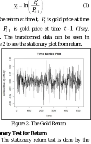
(Tsay, 2002). The transformed data can be seen in Figure 2 to see the stationary plot from return.

Figure 2. The Gold Return Stationary Test for Return

The stationary return test is done by the Augmented Dickey-Fuller (ADF) test. The results of the unit root test can be seen in Table 1.

0

:

1

H

(non-stationary return)

1

:

1

H

(stationary return). Table 1.ADF Test for Return

# Augmented Dickey-Fuller Test Unit Root Test #

p-value: < 2.2e-16

Value of test-statistic is: -16,323 Critical values for test statistics:

1pct 5pct 10pct tau3 -3.43 -2.86 -2.57

According to the test, the null hypothesis is rejected, it means that there is a stationary r e t u r n

return. These stationary return will use in the next step to analyze the heteroscedasticity problems.

Box Jenkins Models

AR (Autoregressive) model with order p denoted by AR (p). The AR (p) for the return at time t

( )

y

_t denoted as

1 1 2 2 ...

t t t p t p t

Y a Y a Y a Y (2)

and the MA (moving average) for the return

y

_t

modeled with this equation.

2

1 1 2 2

...

;

~

(0,

)

t t t t p t q t t

Y

b

b

b

N

(3) For Autoregressive Integrated Moving Average (ARIMA) with orde (p,d,q) denoted as follows.

1 1 1

(1

...

_p p

)(1

)

d _{t t t}

...

p t q

a B

a B

B Y

b

b

(4) where,

(

B Y

j

)

_t

Y

_{t j}is a backward operation. Heteroscedasticity

The residual variance does not change with the change of one or more independent variables. If this assumption is fulfilled, then the residual is homoscedasticity. If the residual variance is not constant, the residual is heteroscedasticity. The heteroscedasticity of residual denoted as follows.

2 1 2

( | , ,..., _k) _i

Var y y y (5)

The problem of heteroscedasticity is an indication of the ARCH (Autoregressive Conditional Heteroskedasticity) effect on the data.

Garch Model

Since the introduction of autoregressive conditional heteroscedasticity (ARCH) models

by Engle (1982), the ARCH and even more related GARCH (Bollerslev, 1986) model have become standard tools for examining the volatility of financial variables. The model has proven to be very useful in capturing heteroskedastic behavior or volatility clustering without the requirement of higher order models in various financial markets.

Autoregressive Conditional Heteroscedasticity (ARCH) with p-order assumed that

2 2 2

1 1

...

t t p t p (6)

With _{t t t}, and _t2 is residual variation at time t.

GARCH is developed to avoid the high orders on the ARCH based on the parsimony principle. GARCH guarantees that the variance is always positive (Enders, 1995).

According to Tsay (2002), let _{t t t}

,

is allowed GARCH (p,q) if 2 2 2 2 2 1 1

...

1 1

...

t t p t p t q t q 2 2 1 1 p q i t i j t j i j (7) where, 2

t = variance of residual at time t

= constant variable

i = ARCH parameter

2 1

t = square of residual at time

t

1

j = GARCH parameter

2

t j= variance of residual at time

t

j

t t t 0

~

(0,1),

0,

0 for

1, 2,..., ,

i

N

i

i

p

0 for 1, 2,..., ; 0 1. j j q i j

GARCH (p,q) connects between the residual variance at t time and the residual variance at the previous time.

RESULT

Box Jenkins’s Models

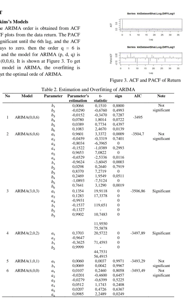
The ARIMA order is obtained from ACF and PACF plots from the data return. The PACF plot is significant until the 6th lag, and the ACF plot decays to zero. then the order q = 6 is obtained and the model for ARIMA (p, d, q) is ARIMA (0,0,6). It is shown at Figure 3. To get the best model in ARIMA, the overfitting is done to get the optimal orde of ARIMA.

Figure 3. ACF and PACF of Return Table 2. Estimation and Overfitting of ARIMA

No Model Parameter Parameter’s estimation

t-statistic

sign AIC Note

1 ARIMA(0,0,6) 0,0066 -0,0290 -0,0152 0,0780 0,0389 0,1083 0,1510 -0,6760 -0,3470 1,8014 0,7734 2,4670 0,8800 0,4993 0,7287 0,0722 0,4397 0,0139 -3495 Not significant 2 ARIMA(6,0,6) 0,9601 -0,0459 -0,8034 -0,1522 0,9653 -0,6529 -0,9624 0,0298 0,8370 0,2469 -1,0893 0,7641 3,3372 -0,3319 -6,3965 -1,0389 7,0822 -2,5336 -3,6045 0,2640 7,2719 1,9549 -7,5124 3,1290 0,0009 0,7401 0 0,2993 0 0,0116 0,0003 0,7919 0 0,0511 0 0,0019 -3504,7 Not significant 3 ARIMA(3,0,3) 0,1354 0,1283 -0,9931 -0,1537 -0,1327 0,9902 19,9118 17,3378 -119,651 -10,7483 -11,9550 75,5878 0 0 0 0 0 0 -3506,86 Significant 4 ARIMA(2,0,2) 0,3703 -0,9647 -0,3625 0,9999 20,5722 -71,4593 -44,7531 56,4915 0 0 0 0 -3497,89 Significant 5 ARIMA(1,0,1) 0,0060 0,0069 0,0037 0,0042 0,9971 0,9967 -3493,29 Not significant 6 ARIMA(6,0,0) 0,0107 -0,0201 -0,0279 0,0512 0,0207 0,0985 0,2460 -0,4600 -0,6399 1,1743 0,4726 2,2489 0,8058 0,6457 0,5225 0,2408 0,6367 0,0249 -3493,49 Not significant

RESUL

The ARIMA model (2,0,2) and ARIMA (3,0,3) have a significant parameter coefficient, so the diagnostic test procedure is continued.

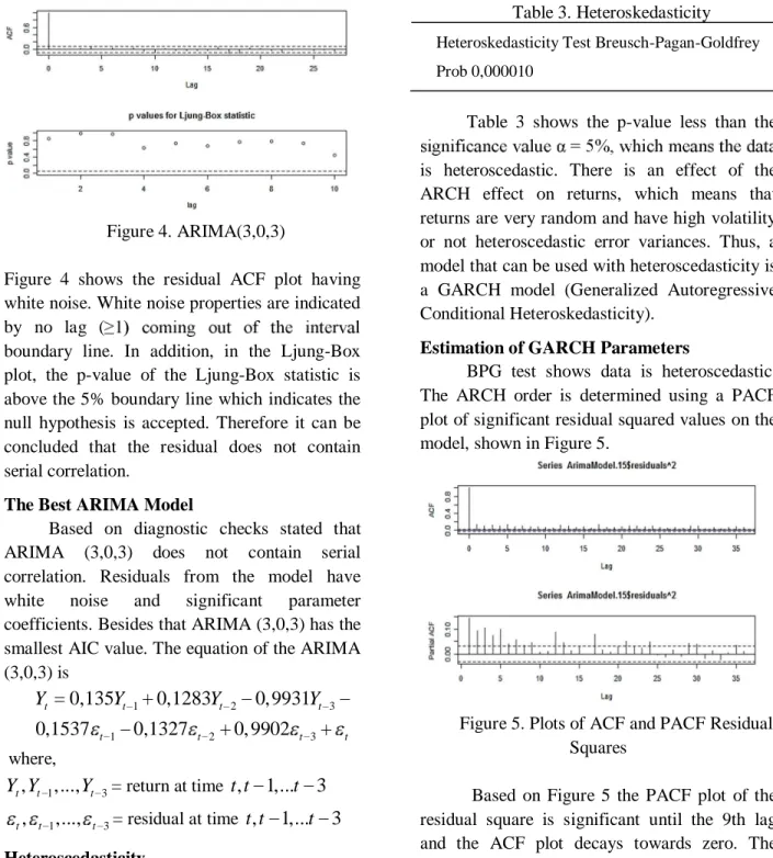
Figure 4. ARIMA(3,0,3)

Figure 4 shows the residual ACF plot having white noise. White noise properties are indicated by no lag (

boundary line. In addition, in the Ljung-Box plot, the p-value of the Ljung-Box statistic is above the 5% boundary line which indicates the null hypothesis is accepted. Therefore it can be concluded that the residual does not contain serial correlation.

The Best ARIMA Model

Based on diagnostic checks stated that ARIMA (3,0,3) does not contain serial correlation. Residuals from the model have white noise and significant parameter coefficients. Besides that ARIMA (3,0,3) has the smallest AIC value. The equation of the ARIMA (3,0,3) is 1 2 3 1 2 3

0,135

0,1283

0, 9931

0,1537

0,1327

0, 9902

t t t t t t t t

Y

Y

Y

Y

where, 1 3

,

,...,

t t t

Y Y

Y

= return at time

t t

,

1,...

t

3

1 3

,

,...,

t t t = residual at time

t t

,

1,...

t

3

Heteroscedasticity

The heteroscedasticity test is carried out by Breusch Pagan Godfrey's test (BPG test)

with hypothesis testing as follows. 0

H

= data is homoscedastic

1

H

= data is not homoscedastic

Table 3. Heteroskedasticity

Heteroskedasticity Test Breusch-Pagan-Goldfrey Prob 0,000010

Table 3 shows the p-value less than the

is heteroscedastic. There is an effect of the ARCH effect on returns, which means that returns are very random and have high volatility or not heteroscedastic error variances. Thus, a model that can be used with heteroscedasticity is a GARCH model (Generalized Autoregressive Conditional Heteroskedasticity).

Estimation of GARCH Parameters

BPG test shows data is heteroscedastic. The ARCH order is determined using a PACF plot of significant residual squared values on the model, shown in Figure 5.

Figure 5. Plots of ACF and PACF Residual Squares

Based on Figure 5 the PACF plot of the residual square is significant until the 9th lag and the ACF plot decays towards zero. The ARCH model with order 9 or ARCH (9) is obtained. However, we can use the GARCH

(p,q) model with a small order of p and q ( e to large order ARCH models.

Selection of the best GARCH model

The best model based on the smallest AIC value with a significant parameter is the ARIMA (3,0,3)-GARCH (1,1) model.

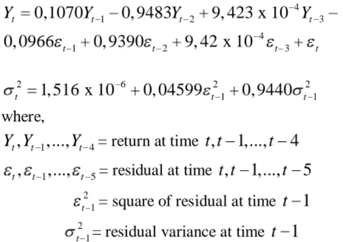
The ARIMA (3,0,3)-GARCH (1,1) model equation is 4 1 2 3 4 1 2 3 0,1070 0, 9483 9, 423 x 10 0, 0966 0, 9390 9, 42 x 10 t t t t t t t t Y Y Y Y 2 6 2 2 1 1 1, 516 x 10 0, 04599 0, 9440 t t t where, 1 4

,

,...,

t t t

Y Y

Y

= return at time

t t

,

1,...,

t

4

1 5

,

,...,

t t t = residual at time

t t

,

1,...,

t

5

_t2₁= square of residual at time

t

1

_t2₁= residual variance at time

t

1

The gold return at time t is influenced by the value of return and residual at time t-1 to t-3. The residual variant at time t is influenced by the residual square at time t-1 and the residual variant at time t-1.

The Accuracy

Forecasting accuracy using MAPE (Mean Absolute Prediction Error). MAPE criteria from sample data of 3%. The prediction of the next period's gold return can be seen in Figure 6.

Figure 6. Original Data vs. Predictive Data

The future return of gold is predicted increasing by time following ARIMA (3,0,3) and the volatility model followed GARCH (1,1).

The model obtained can be used to predict the future gold return. ARIMA (p,d,q) used for predicting the future return and GARCH (p,q) determined the behavior of the volatility. From this study, we knew that ARIMA (3,0,3) and GARCH (1,1) are the best models.

REFERENCES

Bollerslev, T. (1986). Generalized autoregressive conditional heteroscedasticity. Journal of Econometrics, 31, 307-327.

Bollerslev, T., Engle, R. F., & Nelson, D. B. (1994). ARCH models, Econometrics, 4, 2961-3031. Accessed from http://public.econ.duke.edu/~boller/Publishe d_Papers/ben_hand_94.pdf.

Enders, W. (1995). Applied econometric time series. Canada: Jhon Wiley & Sons, Inc.

Engle, R. F. (1982). Autoregressive conditional heteroscedasticity with estimates of the variance of United Kingdom inflation. Econometrica, 50 (4),987-1008.

Marvillia, B.L. (2013). Pemodelan dan peramalan penutupan harga saham PT.TELKOM dengan metode ARCH-GARCH. MATHunesa, 2(1). Accessed from http://jurnalmahasiswa.unesa.ac.id/index.php /mathunesa/article/view/1372.

Ramadhan, B.A. (2015). Analisis perbandingan metode ARIMA dan metode GARCH untuk memprediksi harga saham. E-Proceeding of Management, 2(1). Accessed from http://repository.telkomuniversity.ac.id/pusta ka/files/100199/jurnal_eproc.

Trück, S. & Liang, K, (2012). Modeling and forecasting volatility in the gold market. International Journal of Banking and Finance, 9(1), 48-80.

Tsay, R. S. (2002). Analysis of financial time series 2nd edition. New Jersey: John Wiley & Sons.Inc.

Tully, E. & Lucey, B., (2007). A power GARCH examination of the gold market

ScienceDirect: Research in International