ELECTRICAL ENGINEERING
A flower pollination algorithm based automatic
generation control of interconnected power system
Satya Dinesh Madasu
*, M.L.S. Sai Kumar, Arun Kumar Singh
National Institute of Technology Jamshedpur, India
Received 13 November 2015; revised 24 May 2016; accepted 8 June 2016
KEYWORDS Flower pollination; Weights;
Dynamic loading; Automatic generation con-trol;
Two area thermal system; Governor dead-band nonlinearity
Abstract This paper presents the design and performance analysis of Flower Pollination Algo-rithm (FPA) based Proportional Integral Derivative (PID) controllers for Automatic Generation Control (AGC) of an interconnected power system. A two area thermal system with governor dead-band nonlinearity is considered for the design and analysis purpose. A different kind of approach is made to design a multi-objective function which contains weighted performance func-tions such as ISE, IAE, ISTE, ITAE. These weights are the funcfunc-tions of system response. It is noticed that the dynamic performance of new objective optimized PID controller is better than the others mentioned in the literature. The objective function also includes performance response for various percentage of loads, so that obtained gain parameters are optimal for dynamic load con-ditions.
Ó2016 Ain Shams University. Production and hosting by Elsevier B.V. This is an open access article under the CC BY-NC-ND license (http://creativecommons.org/licenses/by-nc-nd/4.0/).
1. Introduction
The power system is a large-scale network which contains a large number of generators interconnected through the trans-mission network. In this system, the amount of power gener-ated is consumed at the same instant. Any deviation of power causes frequency imbalance in the system network, where frequency is one of the parameter indexes of an AC net-work which is sensitive to load imbalance. So the frequency of
power system is important performance signal to the system operator for stability and security point of view. The primary response of a power system after a disturbance is mainly accomplished by power plants through their speed governor characteristics and load-frequency response. On the other hand, the secondary control in a power system is performed by some units that are equipped with automatic controller which changes the speed governor set points[1]. The primary objective of the AGC is to regulate frequency at specified nom-inal value and maintain the power exchange between the con-trol areas at the scheduled values by adjusting the generated power of specific generators. The combined effects of both the tie line power and the system frequency deviation are gen-erally treated as controlled output of AGC known as Area Control Error(ACE). As the ACE is adjusted to zero by the AGC, both frequency and tie-line power errors will become zero[2,3].
* Corresponding author at: Department of Electrical & Electronics Engineering, NIT Jamshedpur, Jharkhand 831014, India.
E-mail address:[email protected](S.D. Madasu). Peer review under responsibility of Ain Shams University.
Production and hosting by Elsevier
Ain Shams University
Ain Shams Engineering Journal
www.elsevier.com/locate/asej
www.sciencedirect.com
Optimal control techniques such as Genetic Algorithm (GA), Particle Swarm Optimization (PSO), Fuzzy Logic Con-troller (FLC), and Artificial Neural Network (ANN), have been proposed for Load Frequency Control[4–9]. Controller for AGC is developed in two ways. One of them is self-tuning technique which uses the neural network and fuzzy logic controllers and is adopted by group researchers while others follow suitable optimization algorithms. Fuzzy logic based PID controller can be implemented for all non-linear systems but there is no specific mathematical formulation to decide the proper choice of fuzzy parameters (such as inputs, scaling factors, membership functions, and rule base) [10]. From literature survey the enhancement of power system per-formance not only depends on control structure but also on well-tuned controllers. For this purpose, a number of artificial optimization techniques are utilized. So a new high-performance heuristic optimization algorithm is always wel-come to solve real world problems. Flower Pollination Search Algorithm (FPA) is a newly developed heuristic optimization method based on Pollination of flowers.[11–14]illustrate that FPA has the better quality solution, and robustness than other published methods and also has shown considerable domina-tion over GA. It has only one key parameterp(switch proba-bility) which makes the algorithm easier to implement and faster to reach optimum solution[15]. FPA has special capabil-ities such as extensive domain search with quality and consis-tency solution. So it is utilized along with DE for multi-objective optimal dispatch problem [16]. FPA is compared with numerous algorithms[17]and its performance encourages to implement for present problem.
The rest of this paper is organized as follows. Section 2 details the type of power system and their parameters
consid-ered for investigation. The FPA is described briefly in section 3, while Section4deals proposed approach and Section5is presented with results and discussions. Finally, Section 6 shows the conclusions of work.
2. System understudy
The primary objective of the Automatic generation control (AGC) is controlling the power system frequency to the speci-fied nominal value for small perturbation in load. Consider sys-tem ofFig. 1which consists of interconnected power system with two thermal plants. Each one equipped with the non-reheat turbine and a governor modeled along dead band non linearity. These areas are connected through a tie line and whole system is under investigation. FromFig. 1,B1andB2 are fre-quency bias parameters; ACE1 and ACE2 are area control errors;u1 andu2 are the control outputs from the controller; R1 andR2 are the governors speed regulation parameters in p.u. Hz;TG1andTG2are the speed governor time constants in seconds;DPG1andDPG2are the changes in governor valve posi-tions (p.u.);TT1 andTT2 are the turbine time constants in sec-onds; DPT1 and DPT2 are the changes in turbine output powers; DPD1 andDPD2 are the load demand changes;DPTie
is the incremental change in tie line power (p.u.); KPS1 and KPS2are the power system gains;TPS1andTPS2are the power system time constants in seconds;T12is the synchronizing coef-ficient andDf1andDf2are the system frequency deviations in Hz. The relevant parameters are given inAppendix. The trans-fer function of governor with nonlinearity is given by[18]
Gg¼
0:80:2
p s
1þsTg
ð1Þ
3. Overview of flower pollination search algorithm
Flower Pollination Algorithm (FPA) was developed by Xin-She Yang in 2012[19], inspired by pollination of flowering plants. FPA with multi-objective optimization function is uti-lized for controller design [20,21]. Flower pollination is an activity involving the transfer of pollen among the flowers. This takes place typically in two ways. First One through self-pollination (or) local pollination is a biotic form, which contributes 10% of pollination where no pollinators are required. The second one through cross pollination (or) global pollination is an abiotic form which involves pollinators such as insects, birds, bats and other animals, and contributes 90% of pollination. This phenomenon involves agents such as pollinators that move from one flower to other flowers exhibiting a foraging behavior with a pollinator moving more
Figure 2 FPA chart.
0.1 0.2 0.3 0.4 0.5 0.6 0.7 0.8 0.9 1 5 10 15 20 25 30 35 Parameter (p) Global Minima
Figure 3 Change in global minima with respect to parameterp of FPA. 10 20 30 40 50 60 70 80 8 10 12 14 16 18 20 22 24 No of Iterations Global Minima
Figure 4 Change in global minima with respect to number of iteration of FPA.
frequently to certain flowers than others. The frequency of visit to a flower is indicated by term flower constancy. The pro-posed flower pollination algorithm is depicted through flow-chart as shown inFig. 2.
From the flowchart, it is evident that initial step of this algorithm deals with the selection of population size (N) and a parameter (p) which help to decide the amount of self-pollination and cross self-pollination to take place. The algorithm continues by initializing specified number of population (N), with each one containing a group of variables which are opti-mized using the objective function. This algorithm contains an indexing term called flower constancy for each population which determines how well their variables minimize the objec-tive function. Based on the flower constancy, population are queued and best among them is found.
FPA proceeds through generation of new population based on the parameterp, which decides whether this population is generated through self-pollination (or) cross pollination. This is carried out by generating a random variable between 0 and 1 and comparing withpi.e., if the random variable is less thanpglobal pollination takes place (or) else local pollination occurs. For global pollination, agents would move with a dif-ferent step size of length from one flower to another, which is mimicked by levy distribution of flight[22,23]and mathemat-ically represented as(2) LkCðkÞsinð pk 2Þ k 1 s1þk; ðss0>0Þ: ð2Þ The new population generated through global pollination is given by Eq.(3). xtþ1 i ¼x t iþcLðkÞðgx t iÞ ð3Þ wherext
iis the pollenior solution vectorxiat iterationtandg
is the current best solution found among all population at the current iteration. Herecis a scaling factor to control the step size andLðkÞis a step-size parameter that corresponds to the strength of the pollination and a standard gamma function. The local pollination occurs within a small neighborhood of the current population. So its step size ‘’ is taken from a
uni-form distribution. The mathematical expression for such an operation is expressed as(4) xtþ1 i ¼x t iþ x t jx t k ð4Þ wherext j andx t
kare pollen from different flowers of the same
plant species.
Flower constancy for the new population is found in a sim-ilar manner as stated before. If new population flower con-stancy is better than the previous population, they are updated in the position of the previous one (or) else discarded. This process of generation and comparison will continue until the count reachesN. The best among the current population is found and declared as current global best. This process repeats for a maximum number of iterations as specified. The current global best is declared as best solution.
4. The proposed approach
Over the past decades, many control strategies have been pro-posed for AGC, viz. Proportional and integral (PI), and
Pro-10 20 30 40 50 60 70 80 9 10 11 12 13 14 15 No of Population Global Minima
Figure 5 Change in global minima with respect to population of FPA. 0 0.1 0.2 0.3 0.4 0.5 0.6 0.7 0.8 0 2 4 6 8 10 12 14 16 18 20
Magnitude of weights of objective functions
Frequency of weights
IAE ISE ITAE ITSE
Figure 6 Magnitude of weights of objective functions Vs frequency of weights. 0 0.5 1 1.5 2 −0.8 −0.6 −0.4 −0.2 0 0.2 0.4 0.6 Time(s) Δ f 1 (Hz)
Figure 7 Discrete response from proposed model for Df1Vs time.
portional, Integral and Derivative (PID).[24]. In this paper, PID controllers are used to improve the dynamic performance of AGC for a two area thermal power system. The PI, PID control action depends onKP;KI;KDgains which vary for
dif-ferent applications. The tuning of these variables depends on the desired responses of the system. The main function of AGC is to control load frequency and tie line power during load disturbance. So the error signals of frequency and tie line power are used as design criteria to tune the PID controller. The error inputs to the controllers are the respective area con-trol errors (ACE) given by Eqs.(5) and (6):
e1ðtÞ ¼ACE1¼B1Df1þDPTie ð5Þ e2ðtÞ ¼ACE2¼B2Df2þDPTie ð6Þ
The control inputs of the power systemu1andu2with PID structure are given by Eqs.(7) and (8):
u1¼KP1ACE1þKI1 Z ACE1þKD1 dACE1 dt ð7Þ u2¼KP2ACE2þKI2 Z ACE2þKD2 dACE2 dt ð8Þ
The controllers in both the areas are considered to be identical i.e.,KP1¼KP2;KI1¼KI2;KD1¼KD2. In this work, flower pol-lination algorithm (FPA) which is described in Section3 is used to tune the PID controller for a two area Interconnected system. Proportional gain constant (KP1), Integral gain con-stant (KI), and Derivative gain constant (KD) are considered
as variables describing a population defined in an FPA. FPA requires an objective function which uses the design criteria to calculate the flower constancy of the defined population.
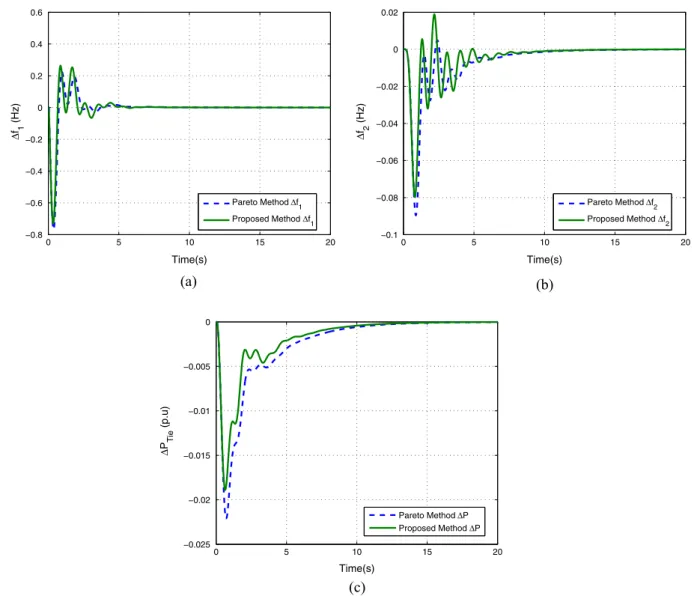
An objective function is created which uses the variables of the population from FPA, passes through a model containing two area thermal system and obtains the error signals fre-quency and tie line power. The performance of these responses is measured using performance functions such as Integral of Absolute Error (IAE), Integral of Squared Error (ISE), Inte-gral of Time multiplied Absolute Error (ITAE), InteInte-gral of Time multiplied Squared Error (ITSE) given by Eqs.(9)–(12) respectively. J1¼IAE¼ Z tsim 0 ½jDf1j þ jDf2j þ jDPTiej dt ð9Þ 0 5 10 15 20 −0.8 −0.6 −0.4 −0.2 0 0.2 0.4 0.6 Δ f1 (Hz) Pareto Method Δf 1 Proposed Method Δf1 Time(s) 0 5 10 15 20 −0.1 −0.08 −0.06 −0.04 −0.02 0 0.02 Δ f2 (Hz) Pareto Method Δf 2 Proposed Method Δf2 Time(s) 0 5 10 15 20 −0.025 −0.02 −0.015 −0.01 −0.005 0 Δ PTie (p.u) Pareto Method ΔP Proposed Method ΔP Time(s) (a) (b) (c)
J2¼ISE¼ Z tsim 0 ðDf1Þ 2þ ðD f2Þ 2þ ðD PTieÞ2dt ð10Þ J3¼ITAE¼ Z tsim 0 ðjDf1j þ jDf2j þ jDPTiejÞ tdt ð11Þ J4¼ITSE¼ Z tsim 0 ½ðDf1Þ2þ ðDf2Þ2þ ðDPTieÞ2 tdt ð12Þ The objective function is designed to consider all the criteria through a weighted sum approach and is given by Eq.(13):
J5¼x1IAEþx2ISEþx3ITAEþx4ITSE ð13Þ x1;x2;x3;x4 are multiplied with IAE, ISE, ITAE, ITSE respectively to form Eq.(13). All these weights should satisfy the following equations as(14) [19]:
XN i¼1
Dxi¼1; xi>0 ð14Þ
Pareto optimality is generally used for choosing these weights. In this work, following approach is proposed to assign weights to the objective function. For this purpose,
the performance function behavior is studied from[25]. It pre-sents the following conclusions:
(1) The ISE and ITSE functions are appropriate to use for measuring the performance when error value is greater than one and vice versa with IAE and ITAE.
(2) The ITAE and ITSE are good measures when error sig-nal persists for a long time and helps to improve steady state error.
(3) While IAE and ISE are useful to mitigate the initial tran-sients, they are used when the transient time is less than one second.
The desired responses that are observed represent all situa-tions, mentioned above, highlighting the fact, that which one of the above performance criteria is best suited for specific time intervals, from a control point of view.
Objective function receives a response from proposed model for a population in FPA. This response is divided for a small interval of step time. A condition is created to imple-ment the conclusions of performance criteria. This condition helps to assign the highest value toDxjiwhenjth performance
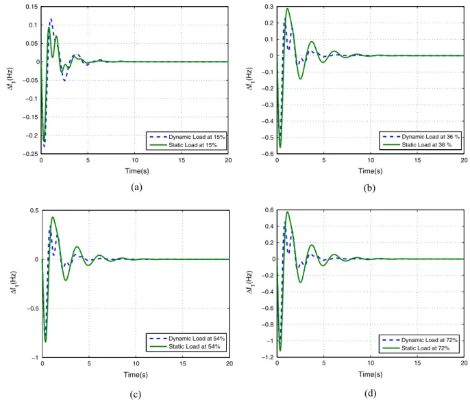
0 5 10 15 20 −0.25 −0.2 −0.15 −0.1 −0.05 0 0.05 0.1 0.15 Δ f1 (Hz) Dynamic Load at 15% Static Load at 15% Time(s) 0 5 10 15 20 −0.6 −0.5 −0.4 −0.3 −0.2 −0.1 0 0.1 0.2 0.3 Δ f1 (Hz) Dynamic Load at 36 % Static Load at 36 % Time(s) 0 5 10 15 20 −1 −0.5 0 0.5 Time(s) Δ f1 (Hz) Dynamic Load at 54% Static Load at 54% 0 5 10 15 20 −1.2 −1 −0.8 −0.6 −0.4 −0.2 0 0.2 0.4 0.6 Δ f1 (Hz) Dynamic Load at 72% Static Load at 72% Time(s) (a) (b) (c) (d)
criteria are best suited for step time, while the others are assigned with minimum values. Later the xj are found from
Eqs.(15) and (16):
N¼ Total simulation time
Definite time interval step ð15Þ
xj¼ 1 N XN i¼1 Dxji " # j¼1;2;3;4. . . ð16Þ using these weights and Eq.(13)flower constancy for FPA is found. This procedure is carried out for a fixed number of iter-ation in FPA, then weights obtained for total best are chosen as fixed weights (or) optimal weights. The FPA restarts its pro-cedure for finding the solution for PID controller parameters
KP;KI;KD using objective for which now has known weights.
Thus, solution for desired PID controller is found.
In[26–29], the proposed objective function was based on fixed step load perturbation and the obtained controller parameters were optimal at fixed step load. But the system load is dynamic, so there is a requirement to design a con-troller that gives optimal response for various load conditions.
In this paper, the objective function includes responses of var-ious percentage step load changes, so the designed controller parameters give optimal response for most load disturbance.
5. Results and discussions
In this paper a two area thermal system with governor dead band is used to test the proposed theory along with FPA. The simulation is performed by using Matlab 2009A on ai7 processor base with 4 GB ram. From Section3it is evident that FPA has parametersp;N(size of population) anditermax
(maximum number of iterations). The parameterpdefines the amount of local search and global search for FPA. To choose this parameter, the proposed method is simulated for various values and that simulated forpvaries from 0.1 to 1 with step change ofpwith step size 0:01 in the range of 0.1 to 1. A graph is plotted between parameterpand respective global minima as shown inFig. 3.
ThisFig. 3shows that objective function is constantly min-imized between 0.5 and 0.6. This is carried out for a number of times and in each case above condition is true, sopis chosen as
0 5 10 15 20 −0.03 −0.025 −0.02 −0.015 −0.01 −0.005 0 0.005 0.01 0.015 Time(s) Δ f2 (Hz) Dynamic Load at 15% Static Load at 15% (a) 0 5 10 15 20 −0.07 −0.06 −0.05 −0.04 −0.03 −0.02 −0.01 0 0.01 0.02 0.03 Time(s) Δ f2 (Hz) Dynamic Load at 36 % Static Load at 36 % (b) 0 5 10 15 20 −0.12 −0.1 −0.08 −0.06 −0.04 −0.02 0 0.02 0.04 0.06 Time(s) Δ f2 (Hz) Dynamic Load at 54% Static Load at 54% (c) 0 5 10 15 20 −0.14 −0.12 −0.1 −0.08 −0.06 −0.04 −0.02 0 0.02 0.04 0.06 Time(s) Δ f2 (Hz) Dynamic Load at 72% Static Load at 72% (d)
5:5. A Similar case study is done for a maximum number of iteration, and it shows that after 40 iterations count value of global minima remains constant as inFig. 4.
Similarly from theFig. 5we have obtained the parameter population size asN¼30.
The objective function contains multiple performance crite-ria as mentioned in Section3, with(16)a set of combinations created. For each combination weight, the proposed method is evaluated and respective global minima are stored. When this data is fed into Pareto efficiency algorithm it has produced fol-lowing weights. This weight combined together will result in 65,536 permutations. By using constraint Eq.(16), these are reduced to 367. Each combination of these weights is passed through FPA and respective global minima are found and stored. These combinations along with the stored vector of glo-bal minima are passed through Pareto efficiency algorithm and Pareto optimal weights are found½0:14230:30260:12950:4256. These combinations of weights are sorted according to ascend-ing order of global minima. The first 10% of weight combina-tions that yields best global minima are analyzed by plotting their histogram as shown inFig. 6.
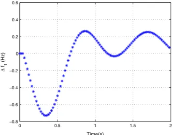
Our proposed techniques as described in Section4would divide the response likeDf1 into definite time interval (0.01 s) as shown in Fig. 7. Suppose at 1:02s the error value is 0:1507 which is less than one and time greater than one. At this point ITAE is best suited for minimizing error, soDxji, ITAE
is assigned with a higher value.
Weights related to ITSE, IAE, ISE are assigned with the lowest value. This is done for theDf2;DPTiesignals. The mean
of step weightsDxji, ITAE for three signals is found. It is
fol-lowed by step weights of other performance function. This procedure is carried out for total simulation time (20 s). Now Eq.(16)is used to find the weightsx1;x2;x3;x4from this step weight vectors. As mentioned in Section4all this procedure is carried out for single population and using Eq.(13)flower con-stancy of the population is found. This is carried out for 20 iterations in FPA then weights obtained for total global min-ima are fixed and are given [0:1255 0:100 0:5796 0:1949]. Fig. 8. shows the response for both methods and it can observed that proposed method has slightly good response when compared to Pareto method. By this proposed method is easy to implement compared to Pareto method.
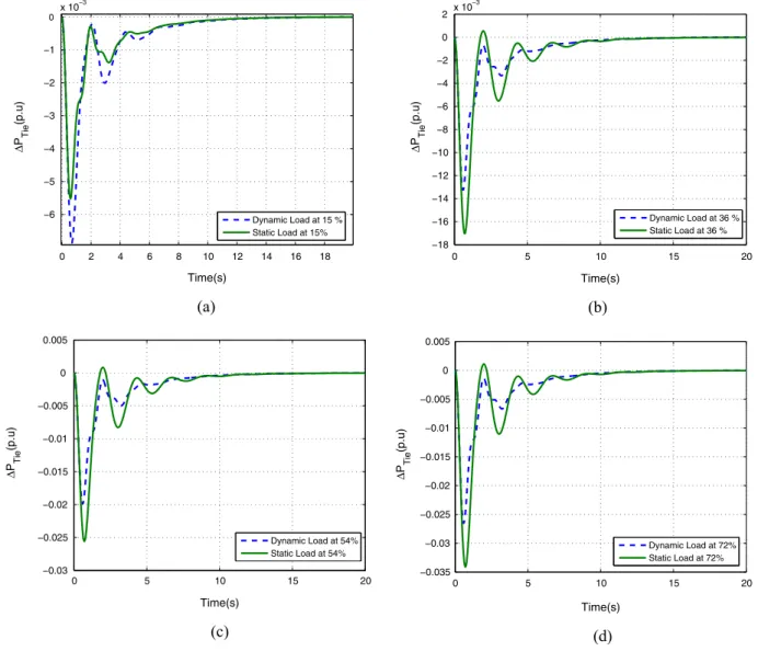
0 2 4 6 8 10 12 14 16 18 −6 −5 −4 −3 −2 −1 0 x 10−3 Time(s) Δ PTie (p.u) Dynamic Load at 15 % Static Load at 15% 0 5 10 15 20 −18 −16 −14 −12 −10 −8 −6 −4 −2 0 2x 10 −3 Time(s) Δ PTie (p.u) Dynamic Load at 36 % Static Load at 36 % 0 5 10 15 20 −0.03 −0.025 −0.02 −0.015 −0.01 −0.005 0 0.005 Time(s) Δ PTie (p.u) Dynamic Load at 54% Static Load at 54% 0 5 10 15 20 −0.035 −0.03 −0.025 −0.02 −0.015 −0.01 −0.005 0 0.005 Time(s) Δ PTie (p.u) Dynamic Load at 72% Static Load at 72% (a) (b) (c) (d)
The second aspect of proposed theory is to construct an objective function which includes a performance for various load percentages (1%, 10%, 30%, 55%, 65%, 80%, 90%) to obtain tuned parameters for a controller of considered system. This yielded gain parameters were optimal for any load change between 1 and 100%. We have tested these gains for 15%, 36%, 54%, 72% load performance. We have also obtained gain parameters tuned for 15% fixed load and test for 36%, 54%, 72% load changes. The comparison of above two perfor-mance is shown inFigs. 9–11 for Df1;Df2;DPTie respectively.
This shows parameters chosen from proposed method are opti-mal for most load changes, so these could give optiopti-mal perfor-mance for dynamic loads also.
6. Conclusion
This study was carried out to design PID controller through Flower Pollination Algorithm (FPA) for Automatic Genera-tion Control (AGC) of an interconnected power system. A two area thermal system with governor dead-band non linear-ity is considered for the design and analysis purpose. A new kind of approach is made to design a multi-objective function which contains weighted performance functions. This method takes less effort to obtain the weights for multi objective func-tion. A single run of the proposed algorithm yields both opti-mal weights and global minimum. The performance of the results is comparable with Pareto optimal solution as shown in Section5. The objective function also includes performance response for various percentage of loads so that obtained gain parameters are optimal for different load conditions and this change could be observed inDf1;Df2;DPTieresponses.
Appendix A. SeeTable 1.
References
[1] Kundur P. Power system stability and control. TMH 8th reprint, New Delhi; 2009.
[2]Elgerd OI. Electric energy systems theory: an introduction. New Delhi: TMH; 1983.
[3]Kothari DP, Nagrath IJ. Modern power system analysis. 4th ed. New Delhi: TMH; 2011.
[4]Saikia LC, Nanda J, Mishra S. Performance comparison of several classical controllers in AGC for multi-area interconnected thermal system. Int J Electr Power Energy Syst 2011;33 (3):394–401.
[5]Parmar KPS, Majhi S, Kothari DP. Load frequency control of a realistic power system with multi-source power generation. Int J Electr Power Energy Syst 2012;42(1):426–33.
[6]Saikia LC, Mishra S, Sinha N, Nanda J. Automatic generation control of a multi area hydrothermal system using reinforced learning neural network controller. Int J Electr Power Energy Syst 2011;33(4):1101–8.
[7]Ibraheem I, Kumar P, Kothari D. Recent philosophies of automatic generation control strategies in power systems. IEEE Trans Power Syst 2005;20(1):346–57.
[8]Ghoshal SP. Optimizations of PID gains by particle swarm optimizations in fuzzy based automatic generation control. Electric Power Syst Res 2004;72(3):203–12.
[9]Golpira H, Bevrani H. Application of GA optimization for automatic generation control design in an interconnected power system. Energy Convers Manage 2011;52(5):2247–55.
[10]Yesil E, Guzelkaya M, Eksin I. Self tuning fuzzy PID type load and frequency controller. Energy Convers Manage 2004;45 (3):377–90.
[11]Huang S-J, Gu P-H, Su W-F, Liu X-Z, Tai T-Y. Application of flower pollination algorithm for placement of distribution trans-formers in a low-voltage grid. In: 2015, IEEE international conference on industrial technology (ICIT). p. 1280–5.
[12]Oda ES, Abdelsalam AA, Abdel-Wahab MN, El-Saadawi MM. Distributed generations planning using flower pollination algo-rithm for enhancing distribution system voltage stability. Ain Shams Eng J 2015.
[13]Chakravarthy V, Rao PM. On the convergence characteristics of flower pollination algorithm for circular array synthesis. In: 2nd International conference on electronics and communication sys-tems (ICECS). IEEE; 2015. p. 485–9.
[14]Draa A. On the performances of the flower pollination algorithm qualitative and quantitative analyses. Appl Soft Comput 2015;34:349–71.
[15]Abdelaziz A, Ali E, Abd Elazim S. Optimal sizing and locations of capacitors in radial distribution systems via flower pollination optimization algorithm and power loss index. Int J Eng Sci Technol 2016;19(1):610–8.
[16]Dubey HM, Pandit M, Panigrahi B. Hybrid flower pollination algorithm with time-varying fuzzy selection mechanism for wind integrated multi-objective dynamic economic dispatch. Renew Energy 2015;83:188–202.
[17]Dubey HM, Pandit M, Panigrahi BK. A biologically inspired modified flower pollination algorithm for solving economic dispatch problems in modern power systems. Cognit Comput 2015;7(5):594–608.
[18]Gozde H, Taplamacioglu MC. Automatic generation control application with craziness based particle swarm optimization in a thermal power system. Int J Electr Power Energy Syst 2011;33 (1):8–16.
[19]Yang X-S. Flower pollination algorithm for global optimization. Berlin Heidelberg: Springer; 2012.
[20]Yang X-S, Karamanoglu M, He X. Flower pollination algorithm: a novel approach for multiobjective optimization. Eng Optim 2014;46(9):1222–37.
[21]Yang X-S, Karamanoglu M, He X. Multi-objective flower algorithm for optimization. Proc Comput Sci 2013;18:861–8. [22]Vedula VSSSC, Paladuga SRC, Prithvi MR. Synthesis of circular
array antenna for sidelobe level and aperture size control using flower pollination algorithm. Int J Antennas Propagat 2015;2015:1–9.
[23]Lukasik S, Kowalski PA. Study of flower pollination algorithm for continuous optimization. Adv Intell Syst Comput 2015;322:451–9.
[24]Kumar J, Ng K-H, Sheble G. AGC simulator for price-based operation. I. A model. IEEE Trans Power Syst 1997;12(2):527–32. [25]Wade M, Johnson M. Towards automatic real-time controller tuning and robustness. 38th IAS annual meeting. Conference Table 1 Appendix.
Variables Typical value
B1;B2 0.425 p.u. MW/Hz R1;R2 2.4 Hz/p.u. TG1;TG2 0.2 s TT1;TT2 0.3 s KPS1;KPS2 120 Hz/p.u. MW TPS1;TPS2 20 s T12 0.0707 p.u. a12 1
record of the industry applications conference 2003, vol. 1. p. 352–9.
[26]Mohanty B, Panda S, Hota PK. Differential evolution algorithm based automatic generation control for interconnected power systems with non-linearity. Alexandria Eng J 2014;53(3):537–52. [27]Sahu RK, Panda S, Padhan S. A hybrid firefly algorithm and
pattern search technique for automatic generation control of multi area power systems. Int J Electr Power Energy Syst 2015;64:9–23. [28]Sahu RK, Panda S, Padhan S. Optimal gravitational search algorithm for automatic generation control of interconnected power systems. Ain Shams Eng J 2014;5(3):721–33.
[29]Padhan S, Sahu RK, Panda S. Automatic generation control with thyristor controlled series compensator including superconducting magnetic energy storage units. Ain Shams Eng J 2014;5(3):759–74.
Satya Dinesh Madasu received the M.Tech. degree from National Institute of Technology, Jamshedpur, Jharkhand, India, in 2010. He is currently working towards the Ph.D. degree at the Department of Electrical & Electronics Engineering, NIT Jamshedpur, Jharkhand, India. His research interests are Application of Control System in Power and Energy Sys-tems and Non Conventional Energy.
M.L.S. Sai Kumarreceived the B.Tech. degree from Anil Neerukonda Institute of Technol-ogy & Science, Vizag, India, in 2013. He received the M.Tech. degree from National Institute of Technology, Jamshedpur, Jhark-hand, India, in 2015. He is currently working towards the Ph.D. degree in the Department of Electrical & Electronics Engineering, NIT Jamshedpur, Jharkhand, India. His research interests are Automatic Generation Control and Power System Protection.
Arun Kumar Singh received the B.Sc.
Engineering degree from NIT Kurukshetra (formerly REC Kurukshetra), Haryana, India, M.Tech. degree from the IIT BHU (formerly IT BHU), Varanasi, UP, India, and Ph.D. degree from the Indian Institute of Technology, Kharagpur, India. He has been a faculty in the Department of Electrical & Electronics Engineering at National Institute of Technology, Jamshedpur, since 1985. His areas of research interest are in Control Sys-tem, Control System Application in Power and Energy Systems and Non Conventional Energy.