Semantic trajectory compression: Representing urban movement in a nutshell

Archive University of Zurich Main Library Strickhofstrasse 39 CH-8057 Zurich www.zora.uzh.ch Year: 2012

Semantic trajectory compression: Representing urban movement in a

nutshell

Richter, Kai-Florian ; Schmid, Falko ; Laube, Patrick

Abstract: There is an increasing number of rapidly growing repositories capturing the movement of people in space-time. Movement trajectory compression becomes an obvious necessity for coping with such growing data volumes. This paper introduces the concept of semantic trajectory compression (STC). STC allows for substantially compressing trajectory data with acceptable information loss. It exploits that human urban mobility typically occurs in transportation networks that define a geographic context for the movement. In STC, a semantic representation of the trajectory that consists of reference points localized in a transportation network replaces raw, highly redundant position information (e.g., from GPS receivers). An experimental evaluation with real and synthetic trajectories demonstrates the power of STC in reducing trajectories to essential information and illustrates how trajectories can be restored from compressed data. The paper discusses possible application areas of STC trajectories.

DOI: https://doi.org/10.5311/JOSIS.2012.4.62

Posted at the Zurich Open Repository and Archive, University of Zurich ZORA URL: https://doi.org/10.5167/uzh-74660

Journal Article Published Version

The following work is licensed under a Creative Commons: Attribution 3.0 Unported (CC BY 3.0) License.

Originally published at:

Richter, Kai-Florian; Schmid, Falko; Laube, Patrick (2012). Semantic trajectory compression: Repre-senting urban movement in a nutshell. Journal of Spatial Information Science, (4):3-30.

RESEARCHARTICLE

Semantic trajectory compression:

Representing urban movement

in a nutshell

∗

Kai-Florian Richter

, Falko Schmid

, and Patrick Laube

1_{SFB/TR 8 Spatial Cognition, University of Bremen, Germany}

2_{Department of Infrastructure Engineering, University of Melbourne, Australia}

3_{Department of Geography, University of Zurich, Switzerland}

Received: June 06, 2011; returned: September 07, 2011; revised: December 22, 2011; accepted: May 05, 2012.

Abstract: There is an increasing number of rapidly growing repositories capturing the movement of people in space-time. Movement trajectory compression becomes an ob-vious necessity for coping with such growing data volumes. This paper introduces the concept ofsemantic trajectory compression(STC). STC allows for substantially compressing trajectory data with acceptable information loss. It exploits that human urban mobility typically occurs in transportation networks that define a geographic context for the move-ment. In STC, a semantic representation of the trajectory that consists of reference points

localized in a transportation network replaces raw, highly redundant position information (e.g., from GPS receivers). An experimental evaluation with real and synthetic trajectories demonstrates the power of STC in reducing trajectories to essential information and illus-trates how trajectories can be restored from compressed data. The paper discusses possible application areas of STC trajectories.

Keywords: trajectories, moving objects, semantic description, data compression, trans-portation network, chunking, navigation, map matching

1 Introduction

Tracking devices mechanistically capture individual movement as trajectories that consist of a series of positioning fixes. Consecutive fixes are co-located, in the sense that tem-porally neighboringfixes refer to similar positions in space. As a result, trajectory data ∗_{This full paper revises and extends an extended abstract version presented at the poster session of the 11th} International Symposium on Spatial and Temporal Databases, July 8–10, 2009, Aalborg, Denmark [39].

is highly spatiotemporally autocorrelated and can be considered redundant. By contrast, humans plan, perceive, and communicate journeys as legs traveled in geographic space, typically following a street network or using train or bus lines. Especially in urban en-vironments there are few alternatives to following available transportation infrastructure network links. This paper exploits such semantic grounding of urban movement for com-pressing trajectory data. In doing so, the paper addresses the GIScience priority of bridging the “gulf between low-level observational data (fixes) and high-level conceptual schemes (journeys) through which we as humans interpret, understand, and use that data” ( [16], p. 300).

5

3

5

3

6

g

B

straight

(a)

ori

(d)

(b)

ori

dest

A

a

a

g

g

g

e

e

A

C

B

B

B

B

D

E

F

G

H

I

F

A

A

(c)

h

h f

f

dest

ori

dest

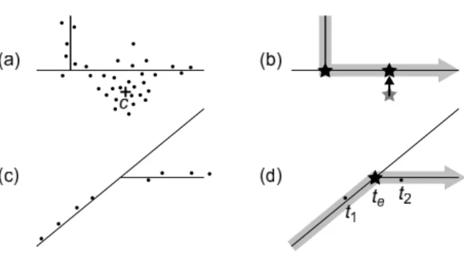
Figure 1: Problem overview (adapted from [39]). (a) Raw positional data asfixes (x,y,t tu-ples); (b) trajectory in two-dimensional space, object moving from origin to destination; (c) trajectory embedded in semantic geographic context; (d) compressed representation of the same trajectory with timestamped reference points as indicated by the clock symbols: from origin, to streetg, streetB, tram line #5, tram line #3,straight, to destination, clock symbols with grey sectors represent intervals.

Consider the trajectory illustrated in Figure 1, which captures the movement of a com-muter from home to work. An array offixes produced by a tracking system (e.g., GPS) is listed in Figure 1a and mapped as a trajectory in Figure 1b. Figure 1c depicts the same

movement embedded in its geographical context. The commuter followed an urban trans-portation network rather than moving in an unconstrained space.

This example illustrates that the observed movement can be modeled by referring to elements of the network semantics. The course can be expressed by the streets and tram tracks it moves along (streetg, streetB, tram line #5, tram line #3) or by references to the movement pattern on the network (straight, to destination). The temporal aspect of the trajectory is captured in the respective timestamps. Figure 1d illustrates this minimalist representation of the observed movement. The use of semantics for trajectory compression exploits related research in thefield of spatial cognition (which is concerned with the ac-quisition, organization, utilization, and revision of knowledge about spatial environments) that aims to design better wayfinding instructions [10, 24, 45].

This paper brings together the reduction of spatial dimensionality of network-constrained movement, the data aggregation potential of semantic information captured in the geographic context of movement, and the theory of wayfinding from spatial cogni-tion. It proposes a novel approach for compressing trajectory data. In detail, the paper advances geographical information science with the following contributions:

• the concept ofsemantic trajectory compression (STC), exploiting the semantic em-bedding of movement for deflating highly redundant trajectory data for an efficient management of movement data;

• the algorithm STC, integrating and extending methods from navigation research (map matching, place identification) and spatial cognition (wayfinding, generation of directions); and

• an evaluation of STC based on a real, example tracking dataset, which has been recorded by GPS in an urban context, as well as synthetic trajectories that have been generated to further explore properties of STC.

STC relies on the availability of transport network data for compression. While this does not cover every type of human movement through space (e.g., hiking in open space national parks), many of today’s trajectory repositories cover movement of (commercial) vehicles or pedestrian movement in urban areas (e.g., motorcycle courier trajectories in London1_{, schoolbus and truck trajectories in the Athens metropolitan area}2_{, or taxi}

trajec-tories in Beijing, as part of the GeoLife GPS data3_).

This article is a full paper version of [39], presented as an extended abstract at the poster session of the 11th International Symposium on Spatial and Temporal Databases, July 8– 10, 2009, Aalborg, Denmark. This full paper presents original work, including a related work section, an elaborated framework of semantics in networks, a detailed description of the proposed algorithms, extensive experimental evaluation sections, and a section on applications of STC trajectories.

2 Related work

Recent work in the areas of database research, spatial cognition, and geographical infor-mation science is particularly relevant to the development of STC. This section provides an

1_{http:!api.ecourier.co.uk} 2_{http:!www.rtreeportal.org}

overview and synthesis of the following four topics: previous work on path and line

simpli-fication; the notion and use of the semantic embedding of trajectories in their geographical context; the use of such semantic information for enriching trajectory data; andfinally, pre-vious work on modeling and querying moving objects in moving object databases (MOD).

Path and line simplification As a reaction to ever increasing volumes of spatiotempo-ral data, recent years have seen initial work on techniques for the compression of such data. With respect to trajectories, the vast toolbox for line generalization appears to offer a quickfix for trajectory compression (e.g., [12]). However, Meratnia and de By [30] argue that conventional spatial line generalization techniques are not suited for spatiotemporal trajectory compression as they ignore temporal aspects in determining the information to retain of the trajectories. Consequently, Meratnia and de By propose alternative geometry-based approaches. Moreover, trajectories are inherently spatiotemporal and compression algorithms should preserve both their spatial and temporal properties. Modeling time as a third spatial dimension, Cao et al. [7] and Gudmundsson et al. [19]—presenting an ap-proximate version of the Douglas-Peucker algorithm—propose path simplification algo-rithms for three-dimensional spaces(x, y, t). Path-simplification is mostly concerned with the question “When is a line segment acceptable as an approximation for a subpath?” which is often tested with some form of tolerance bandε. Additional to shape-preserving algo-rithms, Potamias et al. [32] focus on preserving spatiotemporal features inherent in the trajectory (such as speed or orientation) when subsampling. Both computational geome-try and database communities aim at compression techniques that still allow queries (e.g.,

where at, when at, nearest neighbor) to be answered once the trajectory has been compressed. In general, path-simplification is geometry-driven, be it 2D or 3D. Recently, alternative strategies are discussed that exploit the semantics of trajectories, that is the meaning of a movement path to the moving actors and its embedding in the underlying geography.

Network bound movement The majority of movement planned or performed by humans is bound to some form of network, be it an urban street network, a rail network, or even an air traffic network. In recent years, this a priori knowledge is increasingly exploited for the handling of large volumes of trajectory data.

Linking GPSfixes to a network requires map matching, the process of matching a po-sition datum with a map, i.e., identifying the corresponding infrastructure elements for coordinates in a geographic data set. Mostly, GPS coordinates are matched against street data but there are indoor map matching algorithms as well (e.g., for robot navigation). The increasing ubiquity of GPS sensors in vehicles and mobile devices makes it a vivid research area that aims at improving the accuracy of element identification. The simplest form of map matching is a point-to-point approach: a position datum is matched against a vertex of a street network. Point-to-curve algorithms match the estimated position against edges of the network. In street networks they usually provide a higher accuracy, as vertices may be comparably widely spread (see [4, 46] for an overview of these approaches). More sophisticated algorithms consider topological information of the network, traveling con-straints introduced by transportation means, and heading information. These algorithms outperform the simple approaches as they can detect unlikely and impossible network as-signments [5, 6, 18, 33, 34].

Once trajectories are mapped to a network, the spatial dimensionality is reduced, which allows for efficientindexing structuresfor moving objects [27]. For example, Tiesyte and

Jensen [43] exploit a main-memory index structure enabling incremental similarity search for trajectories of vehicles moving on known routes. The key benefit of such reference systems lies in their reduced spatial dimensionality (convoluted arcs are reduced to linear edges), which enable more efficient indexing.

A priori knowledge about objects moving in a network can then further be used for com-pressing trajectories. For example, Cao and Wolfson [6] model movement along a directed graph that consists of nodes representing intersections and connecting edges representing road segments. Instead of storing large amounts of locationalfixes, theirnon-materialized trajectoriesmodel movement as sequences of tuples (on streetpi, at locationli alongpi, at time ti). Since tuples on the same segment can be merged, non-materialized trajectories require less storage data than raw trajectory data.

Exploiting the semantics of movement Going one step further beyond just linking move-ment to a network graph, the embedding of movemove-ment in the underlying geography offers further a priori knowledge exploitable for trajectory compression.

When compressing trajectories beyond pure geometry, activities (e.g., stops) along the traveled paths need to be preserved. Several algorithmic approaches identify such activi-ties (calledplacesfrom here on) within GPS data. Differences in approaches usually stem from the intended application. There are algorithms for detecting place concepts for hu-man behavior learning [29], for diary applications [8], or for wayfinding assistance [38]. However, all of them consider places to be spatiotemporal clusters, i.e., accumulations of positionfixes in a certain region of a certain size. Most algorithms rely on explicit values for the two crucial parameters time and region size (e.g., 10 minutes, 50 square meters) that define the granularity of the detected places. Some algorithms are parameter-free [38], but detect places on afiner resolution which then are post-processed and selected according to their long-term significance. For trajectory compression the prime interest is in detect-ing significant reference points and not in generating familiarity profiles. STC relies on a simplerfixed parameter algorithm [3, 23].

The database community initially focused mainly on the definition of spatiotemporal data types (e.g.,moving pointandmoving regiondata types [22, 47]). Such spatiotemporal data types allow for queries such as “Find cars that stopped today at point_"x, y_#at time

"t_#”). However, queries referring to the semantic meaning of the movement, such as “Find cars which stopped today at the gas station at time_"t_#” cannot easily be answered [47] because this requires data beyond the trajectory, namely a matching between point_"x, y_#

and the geographic feature “the gas station.” For that reason, more recent research builds on conceptual models of movement, exploring techniques for adding semantic information to trajectories in order to facilitate trajectory analysis in different application domains [2].

Semantic trajectory enriching requires application domain knowledge, as the user must specify what spatial features are relevant to the analysis of trajectories [2, 42] (e.g., hotels, touristic places, or stop-over locations of migrating birds). In STC, the context is always the same and, hence, the characterization of reference points can be done in a much more deterministic way.

Querying moving objects Since the late nineties moving object databases (MODs) devel-oped as a special branch of spatiotemporal databases [22]. The key challenge for MODs lies in keeping track of the constantly changing location of moving objects, balancing positional inaccuracy and costly updates [21]. This section reviews several dimensions of queries for

moving objects, allowing a final discussion about querying STC compressed trajectories (see Section 7).

Location-based queries are a first type of moving object query [1], including nearest-neighbor queries(NN, “Given a moving object O1 and an intervali, which other moving

objectOx is closest toO1 duringi?”) andrange queries(“Given a rectangleR and a time t, which moving objectsOxare within Ratt?”). The second type,trajectory queries, refer to the trajectory as a timestamped polyline, includingsimilarity queries(“Which trajectories are similar in shape?”) andparameter queries(“Which trajectories move north?”).

MODs model and querypastas well aspresent and near futuremovement. The latter is es-pecially challenging as it includes the notion of forecasting and querying future positions. The MOST data model (moving-objects spatiotemporal) and the corresponding FTL (fu-ture temporal logic) allow querying present and fu(fu-ture states through the use of dynamic attributes, extended data types that change implicitly over time [22]. MODs consequently feature various query modes, producing different results as time progresses [40]. Instan-taneousqueries are evaluated once, at timet(“Return the bus stops within 2 km from my current position”).Continuousqueries “travel” with the moving object and are a sequence of instantaneous queries re-evaluated for allt!> t(“Return the bus stops within 2 km from my current (and constantly updated) position”). Finally, apersistentquery at time tis a sequence of instantaneous queries on the infinite history starting att(“Retrieve the objects whose speed doubles within 10 minutes”).

Most research on MODs considers movement in an unconstrained Euclidean space. Only recently, the MOD community addressed network-bound movement [21, 31]. Es-pecially relevant for this paper is the work of [31], as the authors adoptNN,range, and

closest-pair(“Find the hotel-restaurant pair within the smallest driving distance.”) queries for spatial network databases.

3 Trajectory and network semantics

Most tracking systems capture the movement of individuals as trajectories. They store lists of timestamped position samples, so-calledfixes, in the form of tuples(x, y, t). In its most simple form atrajectoryis a polygonal line connecting thefixes of a moving individual [20]. Formally, the trajectoryT of a moving objectOover time interval[ti, tj]is described by

TO(i, j) ="(xi, yi, ti),(xi+1, yi+1, ti+1), . . . ,(xj, yj, tj)#.

TOis linear on each interval[ti, ti+1].

The example trajectory in Figure 1 shows an object moving from originorito destination

dest, over a temporal interval from00:00to59:40. Figure 1a lists thefixes of the trajectory, Figure 1b the respective trajectory mapped in two-dimensional space. Note that only a subset of allfixes are listed in Figure 1a.

Amapis a semantically annotated network of edges and nodes. A map represents an urban transportation network, featuring streets, bus, tram, and train lines (see Figure 1c). A map has the following properties:

• Vertices are unambiguously defined, either by IDs or by(x, y)coordinate tuples. • Edges have labels (street name; or bus, tram, train line, e.g.,Bor 3 in Figure 1c).

• Bus, tram, and train lines can (but need not) be superimposed upon the street net-work. Vertices of bus, tram, and train lines are stops and stations; these may be labeled with the stops’ names.

• The labeling of edges and vertices can extend several levels of granularity. An edge may at the same time have a local street name (e.g., “Ostertorsteinweg”) and be part of a national highway system (e.g., “A7”).

Formally, a map is described by:

M = (VT, ET, VG, EG)

VT is a set of topologicalvertices. These are the intersections of a transport network that define the links between the other topological entities. ET is the set of topological edges between the elements ofVT. Most path planning algorithms work on the elements ofVT andET, which is termed thenetwork graph. This is also the graph compression and decom-pression of trajectories mostly work on. For some operations, though, these processes need to use the geometry of the network configuration. This geometry is described byVG, EG, the sets ofgeometricvertices and edges. With these sets the actual layout of spatial entities in the environment is described. Map matching works on the geometric representation of streets (although sophisticated approaches use the topological representation in parallel), and turning angles, i.e., angles between pairs of streets, are determined on this level. For each topological edge there is a corresponding sequence of geometric edges. Topology abstracts from geometry to connectedness. Figure 2 illustrates this. In Figure 2, the topo-logical edgeeT1T2, which connects the topological verticesvT1andvT2, abstracts from the

sequence offive geometric edgeseG1toeG5that describe the course between the geometric

verticesvG1andvG2. Note that topological vertices always coincide with geometric vertices

(the former are a subset of the latter), but topological edges do not need to correspond to geometric edges.

v

v

e

e

e

e

e

e

v

v

Figure 2: Illustration of how topology abstracts from geometry. The topological edgeeT1T2

abstracts from thefive geometric edgeseG1toeG5.

The advantage of a network lies in reducing the dimensionality of a two-dimensional movement space. An object moving in a network can concisely be positioned along edges and at vertices through timestamping. Given a semantically annotated map, edges and

vertices can be aggregated according to shared labels. Often, several consecutive edges represent the same street and, thus, share the same label. Tram and bus lines may even extend over large sections of a transport network. In short, STC exploits the high-level reference system that comes with the semantic annotation of the transportation network.

Taking this perspective, streets and tram, bus, or train lines can be viewed asmobility channelsthat moving objects hop on, ride for a while, and hop off again to catch another channel that brings them closer to their destination. Only small quantities of information need to be stored for adequately representing the movement of an object riding such chan-nels. With respect to data compression, this mobility channel metaphor illustrates the po-tential for trimming large amounts of redundantfixes. All that needs to be stored to get an accurate approximation of individuals driving, cycling, or walking through a network are the location and hop-on and hop-off times where an object enters or leaves such a channel (e.g., street intersections or bus stops).

Finally,reference pointsstructure trajectories. These reference points are the spatiotem-poral location of where the relevant actions describing the movement of an object in a network happen. Reference points are structurally modeled as points on the network anno-tated with time intervals. The intervals conflate to a time point when changing the mobility channel can be considered instantaneous (e.g., turning from one street into another). STC considers the following types of reference points, which suffice to describe movement in a network:

• Origin and destination of a trajectory clearly are reference points; they define the spatiotemporal boundaries of the represented movement behavior.

• Street intersections and public transport stops are taken as reference points since here channels may be changed.

• Stops within edges constitute reference points. For instance, these stops may occur when a traveler gets stuck in traffic or decides to interrupt the journey to enter a shop. Such stops are identified asplaceswithin the trajectory and are subsequently treated as reference points. Their identification is further discussed in the next section. To summarize, areference pointis a point on the network with an associated time interval whose position corresponds to one of the following semantic elements: origin, destination, street intersection, public transport stop, place.

4 Semantic trajectory compression

This section gives a detailed description of the semantic trajectory compression (STC) ap-proach. In the following, the algorithms for compression (Section 4.1) and decompression (Section 4.2) of trajectories are explained. Section 5 then presents an experimental evalua-tion of both steps.

4.1 Compression

STC is based on the discussion of network semantics in Section 3. Beyond addressing anno-tated network entities, STC follows a semantic approach in how it interprets the trajectory and utilizes this interpretation for compression. STC transforms the geometry of a tra-jectory into a semantic representation that is inspired by mechanisms employed in giving

route directions as they are identified in research on human spatial cognition [10, 24, 45]. Trajectories are described not just through geometry, but by qualitative descriptions of ac-tions along the network. This way, STC can identify and address structures in the envi-ronment that are only graspable if considering how a human perceives it while moving through it. These structures then allow for reducing trajectory descriptions to their seman-tically relevant cores. Broadly, STC is based on three steps (see Figure 3):

1. In a pre-processing step, identify the relevant reference points along the trajectory. 2. For each reference point, determine all possible descriptions of how movement

con-tinues from here.

3. Based on the descriptions, combine consecutive reference points into sequences of ref-erence points. These sequences are termedchunks[24, 26]. The compressed trajectory consists of sequences of such chunks.

Identification of reference points Next to its spatial layout, the temporal order of its reference points is the most important property of a trajectory. However, not every single datum is important to describe the semantics of network movement. Time and location of changing mobility channels and the places (stops along the way) are sufficient to capture these semantics. In a pre-processing step, map matching identifies the positions of origin, destination, possible channel changes, and places on the network. The spatial part of a mapped trajectory corresponds to apaththrough the network; all intersections are vertices ofVT (see Figure 3, center).

Placesare detected by spatiotemporal clustering, similar to the basic accumulative ap-proach described in [23]. A place is detected if the position lies for a defined time in a defined area (e.g., the signal is for at least ten minutes within an area of 50 meters). The place itself is described by the centroid of all measurements, the spatial center of thefixes assigned to the cluster. This centroid is mapped to the closest network entity, which may be an edge or a vertex. It is treated as a single, outstanding reference point. The time interval for the place is computed by the duration of the cluster. Places are special reference points in that, here, the duration of the cluster is significantly longer than for simple channel-changing reference points or stops at traffic lights. Places mark semantically meaningful stops along the way (e.g., for entering buildings), introducing to a topological map new vertices to represent a place’s location. Figure 4 illustrates this: Figure 4a shows a cluster of positioning signals within temporal and spatial boundaries. In Figure 4b the centroid

cis assigned to the closest network entity (faded-out star mapped on the street segment), introducing a new vertex on the edge the centroid is mapped to.

Channel-changing reference points are annotated with a time point. This point (the timestamp) is interpolated from the timestamps of thefix before and thefix after the ref-erence point. Figure 4c and d illustrate the interpolation of a channel-changing refref-erence point: the reference pointteis computed from the fixest1 andt2, which are before (t1),

respectively after (t2) the channel change.

A simple point-to-point map matching has a complexity ofO(nlogn)if using efficient lookup data structures, such as R-trees or its variants, for finding the points in(VG, EG) that match with a trajectoryfix (note that the lookup data structure has to be built only once for a geographic area in a preprocessing step). Identification of reference points is of linear complexity, and can be integrated into the map-matching process. Interpolation of

5 3 ori dest A a a g g g e e A C B B B B D E F G H I F A A 6 h h f f 5 3 ori dest A a a g g g e e A C B B B B D E F G H I F A A 6 h h f f ((2.6 0.9 00:00) (1.7 1.0 03:43) “g”) ((1.7 1.0 03:43) (1.6 1.9 16:43) “B”) ((1.6 1.9 16:43) (1.7 4.1 36:07) “#5”) ((1.7 4.1 36:07) (2.7 6.1 49:36) “#3”) ((2.7 6.1 49:36) (2.4 6.5 53:58 “D”) ((2.4 6.5 53:58) (0.4 7.6 59:40) “straight”) ((2.6 0.9 00:00) (1.7 1.0 03:43) “g”) ((1.7 1.0 03:43) (1.6 1.9 16:43) “B”) ((1.6 1.9 16:43) (1.6 1.9 16:43) “#5”) ((1.7 2.5 20:48) (1.7 4.1 36:07) “#5”) ((2.2 5.1 42:00) (2.4 5.9 47:19) “#3”) ((1.7 4.1 36:07) (2.2 5.1 42:00) “#3”) ((2.4 5.9 47:19) (2.7 6.1 49:36) “#3”) ((2.4 6.5 53:58) (1.1 7.1 57:33) “straight”) ((1.1 7.1 57:33) (0.4 7.6 59:40) “straight”) ((2.7 6.1 49:36) (2.4 6.5 53:58) “D”) 5 3 ori dest A a a g g g e e A C B B B B D E F G H I B A A 6 h h f f compression co m pre sse d t raj ec tor y pa th w ith e ve nts tra jec tor y o n m ap ev en t i de nti fic ati on map matching chunking ev en t d esc rip tio n rec urs ive se arc h, n ot d ep icte d rec on str uc ted p ath co m pre sse d t raj ec tor y decompression Figur e 3: C omp re ssion– d ec omp re ssion. T h e se m an tic ally annota te d ma p fe atur es a tr ain line #6 with two sta tions; tr am line s #3 an d #5 w ith se v er al sto p s; m ajo r str ee ts (U p p er ca se ) an d m in or str ee ts (lo w er ca se ). No te th at m ap m at ch in g is co n sid er ed a pr epr oc es sin g ste p; n ot e als o th at th e re cu rs ive se ar ch n ee d ed fo r d ec om pr es sio n is n ot d epi cte d .

Figure 4: Handling of time. (a) and (b) illustrate the mapping of place centroids against the network infrastructure. (c) and (d) illustrate the interpolation of timestamps for reference points.

timestamps as shown in Figure 4c, d requires to iterate the matched trajectory once, as does place identification as proposed by [23], for example.

Description of reference points For each reference point, unambiguous descriptions of how to proceed from here are generated. The semantics of the underlying network de-termine these descriptions; this makes use of work on cognitively ergonomic route direc-tions [10,35]. Two types of descripdirec-tions are used for capturing the motion continuation at a reference point (see Figure 3 center): egocentric direction relation and network labels. Ego-centric direction relations express changes of directions in terms of qualitative relations, such asstraight,left, orright. The semantics of these relations depend on the underlying qualitative direction model (STC employs the model of [25]). Labels of network elements identify these elements; changes in the labels indicate movement onto the next element. For example, moving from the third (1.6, 1.9) to the fourth (1.72, 2.5) node in Figure 3 center can be described asstraight,B, ortram #5.

In route directions, several consecutive instructions (describing single intersections as exemplified above) can be subsumed into a single, higher-level instruction (e.g., “turn left at the third intersection” instead of “straight, straight, left”; cf. [26]). For their original pur-pose, these higher-level instructions need to be easily understandable for human wayfi nd-ers. Accordingly, the subsumption process needs to make sure that references within and between instructions are unambiguous and comprehensible. This may leave some redun-dant information in the route descriptions. For example, instructing travelers to go straight for the next 47 intersections imposes a cognitive burden on them that is bound to lead to navigation errors and, thus, this single instruction needs to be broken down to several, more manageable instructions. In STC, these references are not required and, thus, redun-dancy can be removed (the STC algorithm has no problem with counting to 47). Instead of trying to ease the task offinding a way through an environment, the descriptions are optimized for the purpose of compression.

Compression of reference points Spatial chunking exploits the spatial structure of an environment. It combines descriptions for several consecutive segments of a path into a single higher-level description. Spatial chunking was discussed in depth in [24]; there, a

formal framework was defined along with an exhaustive set of chunking principles. The applicability of a chunking principle depends on the type of description at hand.

The spatial part of trajectories can be compressed using spatial chunking. The descrip-tions of movement between reference points used in STC (egocentric direcdescrip-tions and net-work labels) requirenumerical chunking as the chunking principle to use. In numerical chunking chunks combine consecutive reference points as long as the same description is used for them (e.g., “tram line #3” chunk in Figure 3). Put differently, reference points are joined until there is a change in description. For example, as long as a trajectory follows edges with identical labels, all these edges are combined into a single chunk by this label. As soon as the label changes, a new chunk is generated. The aim in compression is to create the minimal number of sequences that describe the spatial footprint of a complete trajec-tory, i.e., the minimal number of chunks. As a consequence, most chunks can be expected to cover a considerable part of the trajectory. Generating this sequence is realized as an optimization problem.

Chunking results in a semantically compact description of a trajectory. The chunks reflect parts of the trajectory where no semantic changes occur, i.e., where an individual moved in a coherent part of the network. The crucial information that needs to be stored in the compressed trajectory iswhereandwhena chunk starts and ends. Furthermore, any sub-sequent restoration of the path exploits the description the chunk is based on. Each chunk is stored as a tuple(start,description). Elementstartis a vertex ofVG with a time interval, i.e., a(x, y, t)tuple. Elementdescription is stored as an ID value that is used to identify elements of the network in a lookup table (e.g., a hash table). Since every chunk ends at the

start-element of its successor, there is no need to store anend-element in a chunk, unless for the last chunk, which also contains the timestamped position of the destination, i.e., where the described movement has stopped. Note that this is a lossy compression with respect to time, since only for those reference points explicitly stored in the compressed trajectory their time interval is retained. It is also lossy in geometry, as it matches individualfixes to vertices and edges of the network.

Algorithm 1 summarizes steps 2 and 3 of the semantic trajectory compression process. Functionget all actionsreturns all possible descriptions for a single reference point, functionchunkfinds the optimal sequence of chunks for the list of reference points (cf. [35]). Functionget all actionsperforms two operations for each reference point. It returns the set of labels of the outgoing edge (the network labels) and it calculates the egocentric direction relation between incoming and outgoing edge, i.e., an angle that is converted to a relation symbol. The union of the label set and the relation symbol represents all possible descriptions for the reference point at hand.

As discussed in [35], computational complexity of optimization is dominated by the number of reference pointsn. Richter [35] introduced two different optimization methods: local and global optimization. Global optimization is guaranteed tofind the optimum, but has exponential complexity ofO(2n−1_{). Local optimization has quadratic complexity,} O(n2_{). While it is not guaranteed tofind the optimal solution, extensive tests showed that}

this happens less than 1% of the time, and that in these cases the sub-optimal solution is only marginally longer [35]. Thus, the functionchunkis implemented using local opti-mization, with computational complexity ofO(n2_{). As this is the dominating function in}

Algorithm 1:The semantic trajectory compression (STC) algorithm.

Data:

reference points: a sequence of reference points along the trajectory;

map: the spatial data semantic compression is performed against.

Result:

compressed: a sequence of chunks, i.e., the compressed trajectory. 1 Setcompressed←∅;

2 Setactionlist←∅; 3 whilereference pointsdo

4 Setactions←get all actions(head(reference points),map); 5 Setactionlist←append(actionlist,actions);

6 Setreference points←tail(reference points); 7 end

8 Setcompressed←chunk(actionlist); 9 returncompressed.

4.2 Decompression

In decompression, the aim is to reconstruct movement through an environment. As dis-cussed before, in the chosen semantic approach, decompression does not restore the origi-nal trajectory, but rather the reference points that define this movement (see Figure 3 right). The reconstructed trajectory contains all information on changes of direction as well as places along the way. For those reference points that are reconstructed in decompression, their timestamp is calculated based on an assumed linear movement behavior between start and end point of a chunk. This reconstructed information is sufficient for most tasks, specifically navigation support and most query-by-location services.

In a nutshell, the decompression algorithm iterates through the sequence of chunks stored in the compressed trajectory. It returns a sequence of vertices ofVG that are a geo-metric representation of the traveled path through the network. For each of these vertices, it calculates a timestamp. In more detail, beginning with the startvertex of a chunk the algorithm adds edges ofEGto the reconstructed trajectory until thestartvertex of the next chunk is reached. To this end, it uses different strategies to determine which edge is to be added; these strategies depend on thedescriptionused for chunking.

Chunks based on the egocentric direction relationstraightare decompressed by adding edges that head in the directionstraight as seen from the previous edge. The direction relations are defined in a qualitative direction model that maps angle deviations between two edges to a direction relation [25]. At the current vertex it is checked which outgoing edges are in relation straightto the incoming edge. Since compression generates unam-biguous descriptions for egocentric directions, there will always be only one such edge. In principle, the same approach is taken for the other kinds of descriptions. However, there might be more than one edge at a vertex that adheres to the same concept (identical labels, e.g., change from streetg to streetB in Figure 3). Therefore, a recursive function tries all candidates, i.e., searches a path from the current vertex to thefinal vertex in which all ver-tices are described by the used concept. At each vertex, only the edges that mightfit at all are tested, i.e., the function excludes the incoming edge (to avoid going back) and all edges that cannot be described by the concept at hand. Thus, even though the recursive function

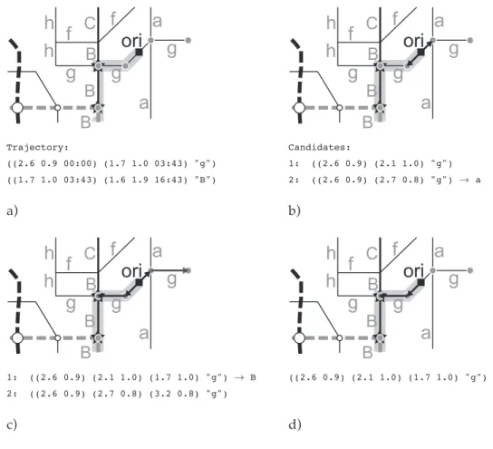
has exponential complexity in theory, in practice the branching factor hardly ever exceeds 2. Figure 5 illustrates decompression based on thefirst two reference points stored in the compressed trajectory of Figure 3.

ori

a

a

g

g

g

C

B

B

B

h

h f

f

ori

a

a

g

g

g

C

B

B

B

h

h f

f

ori

a

a

g

g

g

C

B

B

B

h

h f

f

ori

a

a

g

g

g

C

B

B

B

h

h f

f

Figure 5: Part of the compressed trajectory of Figure 3 (a). Decompression starts at origin

oriand explores both directions along streetg, spanning two alternatives 1 and 2 (b). Al-ternative 2 meets streetain thefirst decompression step (b), alternative 1 meets streetBin the second step (c). According to the sequence of stored reference points (see a), alternative 1 is the correct decompression and is, thus, maintained (d). Note that times are not given in (b), (c), (d) for readability reasons.

Algorithm 2 summarizes the decompression. Decompression needs as input both the compressed trajectory and the map against which compression has been performed.

5 Evaluation

STC has been evaluated using real tracking data and simulated movement data. Both illus-trate the power of the approach for reducing the information that needs to be stored.

Algorithm 2:The decompression algorithm.

Data:

compressed: the compressed trajectory (the result of Algorithm 1), represented as a sequence of chunks;

map: the spatial data compression has been performed against.

Result:

path: a sequence of verticesv∈VGrepresenting the path traveled through the network.

1 Setpath←∅;

2 whilecompresseddo

3 Setcurrentchunk←head(compressed); 4 Setchunkend←segmentend(currentchunk); 5 Setcurrent←segmentstart(currentchunk); 6 Setpartpath←∅;

7 Setadded←true;

8 whileaddedand¬(contains(partpath,chunkend))do 9 Setcandidates←getcandidates(current,map); 10 ifcandidatesthen

11 Setpartpath←probeallcandidates(candidates,map);

/*probeallcandidatesis a function that recursively tries all possible paths to proceed untilchunkendis reached. Fordescription“straight” there is only

one element incandidates. */

12 end

13 else

14 Setadded←f alse;

15 end

16 end

17 if¬(contains(partpath,chunkend))then 18 Setpartpath←∅;

19 end

20 Setpath←append(path,partpath); 21 Setcompressed←tail(compressed); 22 end

23 returnpath.

5.1 Real tracking data

18 everyday trajectories reflecting movement between regularly visited places of four per-sons have been recorded in the city of Bremen with a Garmin eTrex GPS device (sampling rate of 1fix in 10 seconds, positional accuracy varies between 7 to 110 meters; the latter likely indicating positioning errors). The path lengths range from 980 to 7582 meters. Dif-ferent transport modalities were used; the predominant one was traveling by bicycle.

Due to limitations of the used GPS tracking procedure (thefluctuant positional accu-racy) and the subsequent difficulties in correct link identification, the trajectory data had to be preprocessed. The STC compression algorithm uses a trajectory matched to network data as input; in the evaluation, manual correction of wrong matches is sufficient to

demon-(a) (b)

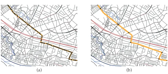
Figure 6: The map shows a part of Bremen where tests have been performed in. As an example, one of the 18 real world trajectories is shown (trajectory #9 of Table 2). The Figure shows in (a) the original trajectory (bold line). The dots represent thefixes mapped to the street network; and in (b) the dots represent the reference points stored in the compressed trajectory.

strate the compression approach itself. In applications dealing with large data sets or real-time map matching (e.g., car navigation systems), the cleaning and map-matching of the data would need to be performed by more sophisticated algorithms as they have been presented in Section 2.

The trajectories were matched onto the map (VG,EG) using a simple point-to-point map matcher. This kind of matcher maps a GPSfix to the closest geometric or topological control point of the curve representing the street [46]. Simple point-to-point matchers are prone to matching errors as they assign thefix to the closest control point in its vicinity without any other plausibility check, such as topological constraint checking. Accordingly, the matching process produced some wrongly assignedfixes. Obviously wrong matches were corrected manually and additional syntheticfixes were added where link identification ambiguities occurred. This situation can occur when the satellite reception of the GPS device is limited andfixes with high positional inaccuracy are obtained. With a series of highly inaccurate

fixes is it not possible to determine the exact traveled path; the implementation of recon-struction heuristics is required. TrackR [36], a trajectory visualization software package, was used to this end. Linear spatiotemporal interpolation determined the syntheticfixes. This assumes constant velocity and straight movement along edges. It did not introduce or alter any information beyond resolving matching problems, an issue not in the focus of this paper.

STC has been tested on all recorded trajectories. Figure 6 shows an example. The trajec-tory is 4336m long and comprises 86fixes; the corresponding path in the map has 49 nodes (elements ofVT) and 102 coordinates (elements ofVG). Performing STC yields the 9 items of Table 1. The table lists the descriptions of each item in plain text to better illustrate refer-ences of semantically meaningful elements in the compressed trajectory. In actual storage of the compressed trajectories, these items should be encoded with unique IDs connected to a lookup table in order to make the byte size of a stored element independent of the length of the attached street name. Decompressing the compressed trajectory restores the

path geometry of the trajectory as it had been mapped to (VG, EG). It also keeps those timestamps that are explicitly stored in the compressed trajectory. Despite some minor differences in the restored coordinates (discussed below), the visual appearance of the de-compressed trajectory is indistinguishable from the trajectory shown in Figure 6a and is, therefore, not shown.

((3490410 5882041 00:00) ”straight”) ((3490057 5882110 01:00) ”Stader Strasse”) ((3490187 5882384 01:51) ”Bismarckstrasse”) ((3488862 5882814 05:43) ”Graf-Moltke-Strasse”) ((3488779 5883229 07:04) ”Hollerallee”) ((3488349 5883565 08:35) ”Am Stern”) ((3488305 5883598 08:47) ”Hollerallee”) ((3487580 5884254 11:31) ”Findorffallee”) ((3487583 5884256 11:32) ”straight” (3487462 5884418 12:05))

Table 1: An STC compressed trajectory.

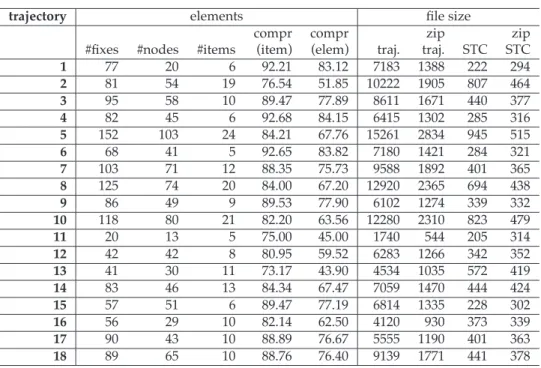
Table 2 summarizes the results of compressing the 18 real world trajectories. The table lists the number offixes of the original trajectory, nodes ofVT after the mapping to the network, and items of the compressed trajectory (corresponding to those listed in Table 1). It also states two compression rates: Thefirst compression rate (“compr(item)”) looks at the number of items of the compressed trajectory (9 for the example of Table 1). The second compression rate (“compr(elem)”) acknowledges that each item comprises two elements (a timestamped coordinate and a description)—except for the last item which addition-ally contains the timestamped coordinate of the destination. Thus, the 9 items of Table 1 correspond to 19 elements. The compression rates state the amount of data reduction, for example, a rate of 89.53 means that 89.53% less data needs to be stored compared to the number offixes of the original trajectory.

The table also compares storage space of trajectory data. It states thefile size in bytes for the original data of the mapped trajectories, thefile size after compressing thesefiles us-ing zip-compression, and thefile size of storing STC-compressed trajectories (both uncom-pressed and zip-comuncom-pressed). Thesefiles are textfiles that simply store one node in each line for the mapped trajectories, respectively one item each line for the STC-compressed trajectories. The comparison with zip-compression allows for evaluating the performance of STC against a (general) lossless compression mechanism.

5.2 Synthetic trajectories

Alongside the real tracking data, the performance of STC was tested using synthetic trajec-tories from simulated movement. Using the same geographical data set that the real track-ing data has been matched to, random paths were calculated on the combined network of streets and tracks. To get paths that are more plausible with respect to human movement through a network space, the approach to simplest paths [13] was used as a path search heuristic. This results in the spatial part of a trajectory; note that this already corresponds to a trajectory mapped to the network, no actual “unmapped” trajectory was generated. The temporal part was simulated by assuming movement with constant speed along the

trajectory elements file size

compr compr zip zip

#fixes #nodes #items (item) (elem) traj. traj. STC STC

1 77 20 6 92.21 83.12 7183 1388 222 294 2 81 54 19 76.54 51.85 10222 1905 807 464 3 95 58 10 89.47 77.89 8611 1671 440 377 4 82 45 6 92.68 84.15 6415 1302 285 316 5 152 103 24 84.21 67.76 15261 2834 945 515 6 68 41 5 92.65 83.82 7180 1421 284 321 7 103 71 12 88.35 75.73 9588 1892 401 365 8 125 74 20 84.00 67.20 12920 2365 694 438 9 86 49 9 89.53 77.90 6102 1274 339 332 10 118 80 21 82.20 63.56 12280 2310 823 479 11 20 13 5 75.00 45.00 1740 544 205 314 12 42 42 8 80.95 59.52 6283 1266 342 352 13 41 30 11 73.17 43.90 4534 1035 572 419 14 83 46 13 84.34 67.47 7059 1470 444 424 15 57 51 6 89.47 77.19 6814 1335 228 302 16 56 29 10 82.14 62.50 4120 930 373 339 17 90 43 10 88.89 76.67 5555 1190 401 363 18 89 65 10 88.76 76.40 9139 1771 441 378

Table 2: Results of the 18 real world trajectories. compr(item) states the compression rate when comparing items of the compressed trajectory; compr(elem) the compression rate for the number of stored elements. File size is given in bytes; “traj.” and “zip traj.” state

file sizes for the (zipped) mapped trajectories, “STC” and “zip STC” for the (zipped) STC compressed trajectories.

path. The speed was randomly set to values between6m

s and14

m

s. A sampling rate of 1fix every 5 seconds was used. Using the speed and sampling rate, the number offixes an ac-tual trajectory along the previously determined path would have was calculated. 1000 such trajectories were created. They vary in length between 1 and 497fixes (mean: 139fixes). Figure 7 illustrates the results of their STC compression. The 1000 trajectories are grouped into ten length classes (shortest 10%, 10% to 20%, . . . ). As for the real tracking data, the number of nodes represents the number of elements ofVT, i.e., the number of topological nodes that describe the movement through the network after mapping the trajectory to the network.

5.3 Results

STC achieves a high compression rate. Looking at the example of Figure 6 again, instead of storing 86fixes, only 9 items need to be stored. This corresponds to a compression rate of 89.53%. Considering the number of elements the compression rate is still 77.90%. As can be seen in Table 2, similar results are achieved for all real world trajectories (mean com-pression rate (items): 85.25%, standard deviation: 6.02; mean comcom-pression rate (elements): 68.98%, st.d.: 12.61). Thesefindings are confirmed by the results of the synthetic trajectories test. STC significantly decreases the amount of data to be stored here as well. Comparing

i t e m s -- n o de

-- f ix e

s

Figure 7: Results for synthetic trajectories. Shown are the number offixes in the original trajectory, nodes in the corresponding path, items in the compressed trajectory. Trajectories have been divided into ten length classes according to the number offixes (lowest 10%, 10–20%, . . . ). The box-whisker plot displays the minimum and maximum of a group (the T-ends of the lines), the interquartile range (the boxes), and the mean number (the horizontal lines in the boxes).

the number of items in the compressed trajectories to the number offixes, on average the compression rate for thefirst group is 77.9%, for the last group 91.4%. Accounting for the fact that two elements (a start reference point and a description) have to be stored in each item, the rates change to 51.8% and 82.4%, respectively. This is still a large reduction.

Matching trajectories to the network already would allow for some compression of the data. In this case only the nodes of the corresponding graph that the matched trajectory passes through need to be stored, annotated with a time stamp of when they are passed. Such an approach, while being simplistic in its implementation, provides an upper bound for the compression rate of the approach by Cao and Wolfson [6]. Figure 7 also shows the compression rates achieved with this method. They range from an average of 29.50% for thefirst group to 61.44% for the last group. This compression is the result of the prepro-cessing step of STC. Performing chunking on the network path (represented by the nodes) by exploiting the semantic information attached to the network’s elements significantly in-creases these compression rates. STC compression is between 20% to 30% higher compared to simple node compression for every group (average 26.76%).

It can also be observed that with increasing number offixes the compression rate in-creases. The longer the trajectories, the better the compression. For very short trajectories (those with 1 or 2fixes only), STC actually creates overhead information as 1fix needs to

be represented using 3 elements (start and end reference point, description). However, the number of STC items increases much slower than the number offixes. The average number offixes in thefirst group is 24.67, in the last group 306.31 (factor 12). The average number of items in thefirst group is 5.45, for the last group it is 26.43 (factor 4.8).

All reconstructed reference points are annotated with estimated timestamps assuming constant speed within a chunk. In some cases decompression returns a path that partially differs from the original path (the trajectory’s realization inVG,EG). For the example of Figure 6, the reconstructed path has 2 coordinates more than the original path. The under-lying geographic data set has individual representations of different lanes for some streets, resulting in different geometric representations. The decompression algorithm may choose to navigate roundabouts clockwise or counterclockwise. These effects may cause differ-ences in the geometric reconstruction of trajectories (see further discussion in Section 8). In the example the reconstruction of movement through the roundabout explains the geomet-ric differences.

The results reported so far compare the number of elements that need to be stored for trajectories. When looking atfile size, i.e., the actual space trajectories take up on storage media, STC also performs well. Zip compressing trajectories certainly results in a signif-icant reduction of storage space—on average a reduction of 80.65% for the 18 trajectories of Table 2. However, STC-compressing these trajectories results in an average reduction of 96.04%. Reducing trajectories to their semantic core, thus, clearly provides a more powerful compression than a simple (syntactic) reduction of the raw data. In fact, it is such a good compression that zip-compressing the STC-compressed trajectories on average results in an increase of storage space again (negative average reduction of₋9.07%).

6 Discussion

There are four main insights that can be drawn from the evaluation: 1) STC compresses trajectories to only a fraction of raw data volumes; 2) it also drastically reduces the amount of data to be stored compared to a trajectory’s network representation; 3) for purposeful movement through a transport network, with increasing length of trajectories, compression increases; the longer a trajectory is, the better is the compression rate; 4) STC reconstructs compressed trajectories featuring all essential information. Highway travel may further illustrate the power of STC. The only information that needs to be stored is the position of ramps on and off the highway and the highway’s name (e.g., a trip on the German interstate A7 from Hannover to Ulm of about 550km, or 6 hours, ideally could be stored using only two information items).

Increasing compression rates with increasing length of trajectories can be explained with the number of direction changes along a path, i.e., those turns at an intersection that are not classified as “straight.” For the tested trajectories, the ratio between the number of nodes in the path corresponding to the trajectory and the number of direction changes is essentially constant over all groups of Figure 7 (between 3.4 and 3.89, no monotone in-crease). Even though with an increasing number of nodes (longer trajectories) the options for turning somewhere increase, longer trajectories representing purposeful movement in a network contain more and longer segments that are chunkable. This can be attributed to the common three-part division of traveling in urban networks [10]: 1) getting from origin on to the system of main streets; 2) traveling along main streets (where only few direction

changes occur); 3) near the end, getting off the main streets again to move to the destina-tion. Due to the chosen path search heuristics in the evaluation, this pattern occurs in the data despite it being random paths.

As explained above, ambiguity may arise in decompressing trajectories. Since label compression does not include heading information, in some situations there may be more than one possible path from start position to end position of a chunk. In such situations, decompression chooses thefirst valid path itfinds. This is due to the fact that STC so far ignores movement modality and associated traffic regulations. Means to account for these are part of future work.

In general, there is a direct relationship between minimizing the stored data in com-pression and an increased effort in restoring the trajectory again. Since only the essential reference points for describing motion in the network are stored, intermediate edges need to be recalculated, which involves resolving possible ambiguities. At the other end of this spectrum every edge that is traversed by the path could be stored, which would take up more space, but would only require an ID lookup. It is also possible to extend the data stored in the tuple representing the chunk. Along with thedescriptionelement (e.g., street name) heading information could be captured; with every change of heading a new chunk would be created. Such a compression would combine at least some reference points and, thus, would be a more compact representation than storing all edge IDs. Decompression then could select that edge at a vertex that is labeled by the used description and heads in the correct direction. However, this paper aims at demonstrating the maximally possible data reduction; a detailed evaluation of the relation between data compression and decom-pression effort is part of future work. Something to note in this context is that even though decompression has exponential run time in theory, in practical terms it runs faster than compression. Due to the low branching factor of the network (street networks are to a most part planar graphs) run time is nearly linear. This is desirable behavior, since in most ap-plications, a trajectory is compressed only once for data storage but may be decompressed several times for further computation.

A specific property of the STC approach is the dependency on having available the same data set for decompression as was used for compression. In contrast to image com-pression procedures, for example, that rely on a “lightweight” comcom-pression algorithm, STC relies on the “heavyweight” input of the (same) semantic data. This is no problem within a single application that either runs on a single machine or is client-server based. And with today’s advances in ubiquitously available spatial data accessible from the web, sharing compressed trajectories across applications and people becomes increasingly easier. It can be expected that in near future (quasi-)standard spatial data emerges that is used in many applications. But even when using a different data set for decompression than for com-pression, the traveled path through the network can likely be reconstructed. Compression is based on semantic information, such as street names or tram lines, and abstracts geom-etry to a qualitative level by using direction relations that correspond to angle intervals. If it is possible to anchor the compressed trajectory in the new data set, i.e., to determine position of origin and initial heading, recovery of the trajectory will be possible using the same methods as described above. Only if the data set for decompression contains less information than the compression set, i.e., if specific layers of information that were used in compression are missing or are incomplete, reconstruction fails. Still, if at least parts of the path can be recovered, it may be possible to use heuristics based on human wayfinding

behavior (e.g., principles identified by [17]) for determining the most probable trajectory to

fill in the gaps.

Another limitation is the dependency on map-matching as a pre-processing step. Map matching algorithms always try to converge toward infrastructural elements. However, humans are not tied to moving exactly along officially mapped streets, they may take short-cuts, like walking straight across a lawn instead of walking around it. A map matching al-gorithm will try to match thefixes to the paths surrounding the lawn. This introduces some error compared to the original movement. Thus, the quality of STC relies on the quality of the applied map matching. Finally, one may argue that reconstructing a trajectory with only interpolated timestamps and not the original trajectory with all its timestamps does not really mirror a full compression-decompression process. However, as previously ar-gued, the reconstructed trajectory represents the semantically meaningful aspects of the movement behavior. Manyfixes, on the other hand, can be expected to be just noise in the movement description that originate from inaccurate localization.

7 Applications of STC trajectories

A major advantage of STC is that the compressed trajectories are human-readable. STC not only compresses streams offixes, but it also transforms raw data into a semantically enriched summary of the movement episodes, not unlike a narrative summary. This opens opportunities for applying STC in a navigation context; trajectories compressed with STC can be used for personalizing mapping and navigation services. For example, personalized navigation assistance as proposed in [37] requires a user model that consists of previously traveled paths and visited places. As STC-trajectories consist of these elements, personal-ized assistance can be directly generated from them.

Thinking this further, the semantic representation of trajectories is ideally suited to com-pare movement within and between different people or objects. For example, checking movement of a specific person in a network for consistency becomes easy, as any major deviation would emerge as differences in the STC compressed representation, while minor (irrelevant) deviations would befiltered out in the compression and, accordingly, would not need to be dealt with. Such comparisons have their applications in areas such as navi-gation services (as discussed above), logistics, or surveillance. Furthermore, it also becomes easily possible to check movement behavior of different people and objects for similarities, for example, to identify people that have similar travel patterns. This has practical applica-tion in areas such as intelligent transport (e.g., identifying opportunities for ride sharing), spatial profile matching, or route optimization in logistics.

Such applications will require querying STC trajectories. Given that STC compresses trajectory data that represents movement in a network environment, there are some differ-ences to the approaches discussed in Section 2.

Trajectory queries STC is all about retaining the relevant semantic information of tra-jectories while reducing redundancies. Since the network elements that tratra-jectories move along are restored in decompression, any queries related to a trajectory’s shape will re-sult in the same rere-sults as if querying the original map-matched trajectory. This holds, for example, for queries, such as: “Where did objectxstop?” “Which trajectories travel in a north-south direction?” “Did objectxmove along network elementy?” Thefirst two

queries can even be answered on the compressed trajectory without a need to decompress again. Also, simple similarity queries can be answered directly using STC trajectories (in-cluding queries, such as “Which other objects follow a similar path to this one?” or “What other objects pass through this network element?”). STC compresses a trajectory into a se-quence representation; therefore, similarity techniques based on quantifying the difference between sequences (e.g., edit distance) present a naturalfit for similarity queries on STC data [9, 11].

Network queries Papadias et al. [31] reformulated queries that are typically run on mov-ing object databases to account for movement in networks. These queries are(k) nearest neighbor, range, andclosest-pair queries. All the queries use network distance instead of Euclidean distance. In order to answer these queries, STC trajectories need to be decom-pressed, except if a query is run using any of the start or end points of any of the chunks as query pointq.

STC trajectories will perform well for any queries that do not require high precision. Queries on STC trajectories are precise to at least the level of edges (as edges are the basic elements of the compression algorithm). Queries, such as “When did objectxpass edge

y?” will deliver useful results since the “objects” moving along the edges usually do not have random speed or acceleration/deceleration patterns, but exhibit consistent patterns. Trains and trams normally move with similar speed patterns, and likewise cars are bound by traffic regulations. However, the STC approach fails to pick up extreme behavior. For example, if an object accelerates and decelerates rapidly between start and end points of chunks, this movement behavior would be impossible to represent and query in a STC trajectory.

Network queries lead to correct results on the level of granularity of network distance from an edge. However,distance from edgeis a more complex operation, with a less clear semantics, thandistance from point. Thus, usually these queries will be run using an inter-polated point qi on that edge. Interpolatedfixes do not need to match with fixes in the original, matched trajectory; this may result in deviations between query results on the original trajectory and the STC trajectory. For example, if two or more objects of the re-quested type have a similar distance to the original pointqo (often, this corresponds to a high density in distribution of that object type), a query using the interpolated pointqimay return the object that is in fact farer away fromqoif the interpolation movesqicloser to that object. Likewise, range queries usingqimay miss some objects on or close to the fringe of the selected range as seen fromqo, or include some that are just missed by a query usingqo. To sum up, STC trajectories perform well for any queries related to trajectory shape and similarity. They will also generally perform well for any queries that do not require very high precision, i.e., where results are expected to be on a granularity level corresponding to edges. These are the kind of queries required for the application areas discussed above.

8 Conclusions and outlook

This paper presents semantic trajectory compression(STC) for compressing large volumes of trajectory data. STC exploits the semantic embedding of movement in a geographical context. It matches individual trajectories to a semantically annotated map and aggre-gates movement chunks based on identical semantic descriptions. STC extends concepts of

network-constrained indexing in moving object databases and techniques used in wayfi nd-ing assistance. This paper’s main contribution lies in illustratnd-ing that the embeddnd-ing of human movement in its geographic context (here an urban transport network) can be ex-ploited for compressing large volumes of raw trajectory data. Initial experiments show that semantic compression achieves high compression rates for real and synthetic trajectories, with arguably acceptable information loss.

As part of future work, movement modality (“walking,” “cycling,” “driving,” “going by tram”) will be explored to improve compression and decompression in STC (cf. [14,41]). Knowing the movement modality allows for an improved identification of reference points. For example, for an individual traveling by train in compression intermediate reference points, where the train stopped at stations, can be ignored and only the positions of the stations where the individual entered and left the train need to be stored as reference points. In decompression, movement modality reduces ambiguity. Traffic regulations restrict the possible edges that movement may have occurred on, dependent on the modality. This would rule out going clockwise through a roundabout when driving a car, for example. Such possible behavior cannot be excluded for pedestrian movement (and may also happen in motorized traffic; see the analysis in [44]). Further ambiguities may be solved by using heuristics accounting for the likelihood for a correct match, for example, based on the travel speed (cf. [28], who use odometry data to exclude unlikely candidates in matching GPS

fixes to a network).

So far, STC was developed primarily with a data compression motivation. Still, some potential application areas of STC-compressed trajectories were suggested. These applica-tions require queries on STC trajectories; their general behavior was discussed. However, querying STC-compressed trajectories demands further analysis and, accordingly, alterna-tive evaluation techniques for STC will be developed. The experiments in Section 5 in-vestigated STC with respect to data compression rate and spatial accuracy, respectively data loss of the compression-decompression sequence. Additional experiments will explic-itly evaluate the spatiotemporal restoration accuracy in a more rigorous way, for example “Where in space and time lies afix of the decompressed trajectory with respect to its coun-terpart in the original uncompressed trajectory?” (cf., e.g., [15] who present an error anal-ysis for time slice queries). One way of assessing this spatiotemporal restoration accuracy is the stochastic analysis of the distance between randomly selected pairs of correspond-ingfixes (decompressed versus original). The compression of a trajectory could be called “spatiotemporally accurate,” if the average spatiotemporal distance between such pairs does not exceed a given threshold. Such evaluation, however, requires more accurate GPS tracks than were available for the present initial study.

Acknowledgments

Support by the German Science Foundation (DFG) and Group of Eight/DAAD Australia Germany Joint Research Co-operation Scheme is acknowledged.

References

[1] AGARWAL, P. K., GUIBAS, L. J., EDELSBRUNNER, H., ERICKSON, J., ISARD, M.,

M., MANOCHA, D., METAXAS, D., MIRTICH, B., MOUNT, D., MUTHUKRISHNAN, S., PAI, D., SACKS, E., SNOEYINK, J., SURI, S.,