Received 30 September 2009, Revised 23 March 2010 Ó 2010, DESIDOC
1. INTRODUCTION
An electronic nose consists of chemical sensor array with pattern recognition system to detect and identify vapour prints of target chemical compounds in gaseous phase. Its applications range from monitoring of hazardous chemicals in the environment, detection of disease through body odour or breathe, smell sensing and monitoring of food degradation through bacterial metabolites emission, to detection of explosives and narcotics through sniffing of the suspects. The detection of trace vapours emanating from hidden explosives is of paramount importance to homeland security and forensics. The security applications include sniffing hidden bombs, landmines, and suspected baggages or persons. The forensic uses involve early identification of devices and contraband activities for prevention of difficult countermeasures later.
However, developing a portable electronic nose technology for these purposes is a difficult task due to extremely low vapour pressure of most of the chemical compounds comprising modern explosives. The vapour pressures at ordinary temperatures of most commonly used pure explosive compounds vary from 10-6 to 10-14 torr 1, 2. For example, the vapour concentration of DNT (dinitrotoluene) is in
ppm (parts per million) range, TNT (trinitrotoluene) in ppb (parts per billion) range, RDX (research development explosive cyclotrimethylene trinitramine) and PETN (Pentaerythritol tetranitrate) in ppt (parts per trillion) range, and HMX (high melting explosiveoctahydro-tetranitro tetrazocine) in ppq (parts per quadrillion) range3. The reliable detection of explosives vapour signature or vapour prints at such low concentrations is a challenging task even for some most advanced detection techniques today3-5. The difficulty is further compounded as the trace explosive vapours are usually camouflaged in complex background of several interfering volatile organic compounds. The compositions of latter vary wildly over various kinds of sites of interest. For example, ambient air over landmines will be drastically different from that near the body of a person boarding an aircraft hiding a bomb or a busy market place threatened with a hidden bomb6,7.
Several alternate sensor technologies have been developed to meet this challenge7-11. The most important of these are based on gravimetric, optical, and chemoresitive principles implemented on varied platforms. The gravimetric sensors based on surface acoustic wave (SAW) platform are perhaps the most sensitive, miniature and rugged of
Development of Surface Acoustic Wave Electronic Nose
using Pattern Recognition System
S.K. Jha and R.D.S. Yadava
*Banaras Hindu University, Varanasi-221 005 *Email: [email protected], [email protected]
ABSTRACT
The paper proposes an effective method to design and develop surface acoustic wave (SAW) sensor array-based electronic nose systems for specific target applications. The paper suggests that before undertaking full hardware development empirically through hit and trial for sensor selection, it is prudent to develop accurate sensor array simulator for generating synthetic data and optimising sensor array design and pattern recognition system. The latter aspects are most time-consuming and cost-intensive parts in the development of an electronic nose system. This is because most of the electronic sensor platforms, circuit components, and electromechanical parts are available commercially-off-the-shelve (COTS), whereas knowledge about specific polymers and data analysis software are often guarded due to commercial or strategic interests. In this study, an 11-element SAW sensor array is modelled to detect and identify trinitrotoluene (TNT) and dinitrotoluene (DNT) explosive vapours in the presence of toluene, benzene, dimethylmethylphosphonate (DMMP) and humidity as interferents. Additive noise sources and outliers were included in the model for data generation. The pattern recognition system consists of: (i) a preprocessor based on logarithmic data scaling, dimensional autoscaling, and singular value decomposition-based denoising, (ii) principal component analysis (PCA)-based feature extractor, and (iii) an artificial neural network (ANN) classifier. The efficacy of this approach is illustrated by presenting detailed PCA analysis and classification results under varied conditions of noise and outlier, and by analysing comparative performance of four classifiers (neural network, k-nearest neighbour, naïve Bayes, and support vector machine).
Keywords: SAW sensor array, electronic nose, TNT vapour detection, SVD denoising, pattern recognition, pattern recognition system, singular valve decompostion based denoising
them all12. Most interesting aspects of SAW sensors are their continuous upgradability in performance through increase in operation frequency13, modification in device design14-17, improvement in polymer interface18, and planar technology19.
The SAW sensor technology has gone through development of nearly three decades and still there remains vast potential to exploit20-22. Some SAW sensor array-based electronic nose products have been launched and many more have been reported from research and development laboratories23-26. Having a fairly mature SAW device technology, the critical bottleneck in the performance of SAW sensor array-based electronic nose systems comes from selection of chemical selective polymer coatings and signal processing for vapour pattern recognition27-32. Most of the electronic components, electromechanical parts and data acquisition systems involved in the construction of an electronic nose system are commercially available. A large number of polymers are also commercially available from which suitably selective ones can be chosen.
However, selection of proper polymers requires experimenting with a large set of potentially useful polymers, either by making sensor arrays in various combinations and evaluating these for target vapour discrimination 27-32 or by alternate thermochemical characterisation such as thermogravimetric analysis, Fourier transform spectrometry, and quartz crystal microbalance-based sorption-desorption analysis33,34. This is quite an expensive and time-consuming process. This apart, the development of an efficient and reliable pattern recognition software for vapour prints extraction and identification is perhaps the most limiting and expensive aspect today35,36. In this paper, the feasibility of using theoretical models of prospective SAW sensor array for both the polymer selection and the vapour recognition tools development with the purpose of reducing the development time and cost of an electronic instrument has been studied.
As a part of this effort, a case study of trinitrotoluene (TNT) detection has been reported by designing a model SAW sensor array coated with a set of polymers whose solvation characteristics are known. The theoretical design also includes an additive Gaussian noise source. Response analyses of some potential interfering gases are also considered. Discrimination of TNT pattern against patterns of interfering gases is studied by applying the singular value decomposition for data denoising, nonlinear principal component analysis for feature extraction, and artificial neural network for pattern classification. The present work outlines and illustrates a prudent approach for the cost-effective development of SAW sensors-based electronic nose. In particular, it is emphasised that the flexibility in generating synthetic data posing different difficulty levels in vapour recognition will greatly facilitate development of pattern recognition tools for specific applications without waiting for real data. Final adjustment and tuning can be done later with real data at much reduced time and cost.
2. SAW SENSOR ARRAY SIMULATION 2.1 SAW Sensor Model
SAW sensors are oscillator circuits whose resonance frequencies are controlled by SAW delay line or resonator devices in the feedback path. The SAW devices are functionalised for chemical vapour sorption by depositing broadly selective polymer thin films in the acoustic wave propagation region. Exposure to vapour generates shift in oscillator frequency, and is taken to be the chemical signal. Theoretical model of polymer-coated SAW oscillator sensors is fairly developed and experimentally validated37. Recently,15 an accurate analytical expression for change in SAW oscillator frequency due to polymer coating and vapour sorption has been developed by approximating the original formulation37, which is quite complex due to several implicit parametric dependencies. The fractional change in SAW oscillator frequency due to polymer coating is given as15 ( ) 1 3 ( ) (2 ) 1 2 3 2 1 3 2 0 0 4 1 2 ' p ' p p p f h c c c c c G h c c G f v G é ù D @ -w r ê + + - + + w r + ú r ê ú ë û (1)
where f0 is the unperturbed SAW oscillator frequency and
p
f
D is the change after coating. The other symbols are: 0
2 f
w = p , h is polymer thickness, rp is polymer density, '
G G iG''= + is the complex shear modulus of the polymer
film, G2 =G'2+G''2, 0
v is unperturbed SAW velocity, and 1
c, c2 and c3 are material constants specific to SAW substrate and propagation direction. For SAW devices on ST-X
quartz, 5 0 3 158 10 v = . ´ cms-1, and 7 1 0 013 10 c = . ´ - , 7 2 1 142 10 c = . ´ - and 7 3 0 615 10 c = . ´ - in units of cm2sg-1. The frequency change after equilibrium sorption of vapour species in the polymer coating (say, Dfv) is obtained
from Eqn (1) by replacing rp by r + Drp v where Drv
represents the change in film density due to vapour sorption. The latter is obtained as Dr =v KCV where K C / C= P V
denotes equilibrium partition coefficient as ratio of the vapour concentration in the polymer (CP)and the gaseous
(CV) phases. The sensor signal is the additional change
in frequency due to vapour sorption, and is obtained as
v p
f f f
D = D - D (2) 2.2 Addition of Noise Sources and Outlier
In operation of real electronic nose systems, some undesired contributions to sensor outputs always appear in the form of noise and/or outliers. The noise contributions arise at each stage involved in the sensor output generation starting from the vapour sampling, transduction, signal generation and analog signal processing to the data acquisition. The combined effect of all noise sources to be additive Gaussian has been assumed. To generate noisy data, the model SAW sensor array output is added to a noise sources having zero mean and standard deviation typical of SAW delay line oscillators with ppm-stabilities.
The model also incorporates additive outliers. Tto do that, an outlier value and probability of its occurrence
were generated by assuming uniform random distributions over different ranges. For example, a frequency outlier value was generated by generating a random value over [-50, +50] Hz, then the probability of its occurrence was assigned by generating another random number over [-1, 1]. The outlier is taken to occur if the probability of its occurrence is greater than a predefined threshold (say, 0.90). The sensor array response matrix is obtained by adding the noise and outlier components to the signal generated by Eqn (2).
3. A MODEL SAW SENSOR ARRAY AND TNT RESPONSE
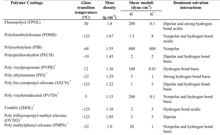
A model sensor array consisting of 11 SAW delay line oscillators coated with different polymers is taken for simulation and analysis. The nominal oscillator frequencies are 200 MHz. The polymers are listed in Table 1. Along with the target vapour TNT, 5 more interferent vapors are also included as listed in Table 2. The selection of polymers has been done by considering the solvation characteristics of analyte vapours and their complimentary characteristics
Shear moduli (dyne cm-2) Polymer Coatings Glass
transition temperature (°C) Mass density (g cm-3) G' G" Dominant solvation interactions Fluoropolyol (FPOL) 30 1.8 200 0.1 Dipolar and strong hydrogen
bond acidic
Polydimethylsiloxane (PDMS) -123 1.67 1.5 8 Nonpolar and hydrogen bond acidic
Polyisobutylene (PIB) -68 1.55 800 800 Nonpolar
Polyepichlorohydrin (PECH) -19 1.45 2 2 Dipolar and hydrogen bond basic
Poly vinylpropionate (PVPR)*
12 1.36 100 0.01 Hydrogen bond basic
Poly ethylenimine (PEI) *
-23 1.29 5 1 Strong hydrogen bond basic Poly bis-cynopropyl-siloxane (SXCN) *
-123 1.22 1 5 Dipolar and hydrogen bond basic
Poly vinyltetradecanal (PVTD) *
5 1.15 200 0.1 Nonpolar and hydrogen bond basic
Fomblii (ZDOL) *
-125 1.10 2 5 Hydrogen bond acidic
Poly trifluoropropyl-methyl-siloxane
(OV202) * -123 1.05 2 5 Dipolar
Poly methylphenyl-siloxane (PMPS) *
-32 1.0 20 1 Nonpolar and hydrogen bond basic
*Note: The shear moduli for the later seven polymers are assumed values.
Chemical
Compounds Vapour pressure at 25 °C (Torr)
Characteristics Trinitrotoluene (TNT) 3.0´10-6 It is a common explosive47
Dinitrotoluene (DNT) 2.1´10-4 It is always present in TNT as impurity, and has significantly higher vapour pressure than TNT47
Dimethyl methyl
phosphonate (DMMP) 1.15 A simulant of chemical weapon agent
48
Toluene (TOL) 21.9 A potential interferent vapour arising from vehicular emission49
Benzene (BNZ) 80.9 A potential interferent vapour arising from vehicular emission49
Water (H2O) 17.5 Universal interferent49
Table 1. Polymer coatings selected for the model SAW sensor array for detection of TNT vapour, and their characteristics28,29,39,40
Table 2. Analyte chemical compounds in vapour phase for detection by model SAW sensor array and their characteristics
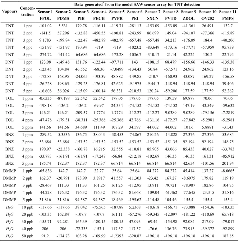
needed in the chemical interface for selective and sensitive vapour sorption. This has been done based on the linear solvation energy relationship (LSER) 38, and using the available solvation parameters in published literature28,29,39,40. The calculated partition coefficient for different vapour-polymer pairs is shown in Table 3. The sensor array output is computed using Eqns (1) and (2) for 30 concentration levels of each analyte vapour. Since the vapour pressure of these compounds varies over a large range under normal conditions as shown in Table 2, their concentrations in the headspace samples of the suspected targets will also vary accordingly. In view of this, the synthetic array response data was generated by varying the concentrations of the different analyte vapours in unit steps from 1 to 30 with units taken to be ppt (parts per trillion) for TNT and DNT, ppb (parts per billion) for DMMP and ppm (parts per million) for benzene, toluene and water. To convert these vapour concentrations from the parts by volume to g/cm3, the normal temperature and pressure conditions are assumed. In this way, a synthetic data matrix of size 180´11 was generated where individual sensors are represented in the columns and the vapour samples in the rows. The noise and outliers were added to the data as explained in the preceding. A typical data matrix for 5 concentrations of each vapour corrupted with additive Gaussian noise and uniformly distributed outliers is shown in Table 4. Here the Gaussian mean is also assumed to be randomly distributed. 4. PATTERN RECOGNITION SYSTEM
The output of individual sensors in the array under action of a vapour sample results from cumulative effect of several molecular interaction processes. The vapour molecules and polymer matrix interact via polar and nonpolar affinities, hydrogen bonding processes and dispersive forces. The LSER models these interactions as a solvation process in which different interaction mechanisms contribute independently, and the total effect results from linear superposition of individual contributions. In the LSER model, each contribution is expressed as product of two solvation parametersone characterising the vapour molecules and the other characterising the polymer. These parameters represent complementary solvation characteristics. For example, the hydrogen bond acidity of vapour molecules and the hydrogen bond basicity of the polymer, or the dipole moment
of vapour molecules and the polarisability of functional groups in polymer. The solvation parameters are the characteristic descriptors of vapour-polymer interactions. The set of all solvation parameters of molecules of a chemical compound in vapour will be unique, and can be taken to represent its mathematical signature.
The outputs of different polymeric sensors in a multisensor array system present varied representations of the vapour solvation parameters. The real vapour samples contain several types of molecules present simultaneously. The exposure to a real vapour sample therefore generates a response vector that is superposition of several sub-responses arising from different types of vapour species. If one labels different real vapour samples by index k, then k kj ik ij ik ij j kj j j j i j i j R c R æ c a sö b s = = = ç ÷ = è ø
å
åå
å å
å
R (3)where cik represents the fractional concentration of i-th
vapour species in k-th sample, and Rij is unit concentration
response of j-th sensor due to i-th species. The response vector for a given vapour sample thus depends on the fractional concentrations and specific sensitivities of different molecular species cik and aij , respectively; s denotej
sensor directions in multi-dimensional data space. Measurements for a set of m samples by n element sensor array can be written in a matrix form
1 11 12 1 1 2 21 22 2 2 1 2 n n m m m mn n R b b ... b s R b b ... b s ... ... ... R b b ... b s æ ö æ öæ ö ç ÷ ç ÷ç ÷ ç ÷ ç= ÷ç ÷ ç ÷ ç ÷ç ÷ ç ÷ ç ÷ç ÷ ç ÷ ç ÷ç ÷ è ø è øè ø (4)
If the vapour samples contain only one compound; if the set of sensors in the array are independent, and if the polymer solvation parameters are known; then Eqn. (4) presents a set of linear algebraic equations which can be solved to determine the set of solvation parameters of vapour molecules. However, this would be an unrealistic idealisation even in most simple applications. Therefore, the sensor array-based measurements can not be used to extract vapour solvation parameters. The goal of a pattern recognition system is to build a set of mathematical descriptors (each being some combination of characteristic solvation
Polymer (Calculated partition coefficient for vapour/polymer pairs) Vapour
FPOL PDMS PIB PECH PVPR PEI SXCN PVTD ZDOL OV202 PMPS TNT 9.918 7.2318 7.9477 9.9765 8.5193 9.975 9.8161 8.3878 7.61 8.6142 8.7322 DNT 7.3324 5.7639 6.1152 7.5025 6.5198 7.657 7.0826 6.4336 5.793 6.5423 6.7481 Toluene 2.4072 3.0662 2.7658 3.0168 2.8025 3.4881 2.1887 2.8726 2.251 2.7902 3.1599 Benzene 1.9646 2.6129 2.2153 2.5704 2.4204 3.0775 1.7736 2.3765 1.8616 2.3493 2.6961 DMMP 6.3804 3.765 3.576 4.5009 3.964 4.2715 3.7459 3.8568 5.6477 4.3799 4.0997 Water 2.3064 1.3397 -0.191 1.6368 2.1962 6.4792 2.2628 2.06 2.4344 1.0149 1.4053 Table 3. Equilibrium partition coefficients (log K) calculated using LSER model and the solvation
descriptors) from the multisensor data such that they represent the vapour identity in unique manner. It can be noted that the set of characteristics sensitivities aij itself would be
unique to different molecules. Therefore, they would suffice to define the molecular signature. However, extracting them from Eqn. (4), where relative concentrations of different species are not known, is almost impossible. Therefore, the statistical estimation procedures make the bedrock of most pattern-recognition algorithms. This necessitates
generating data with known vapour samples (called training data) first, and established the statistical estimation methods of signature building in supervised mode.
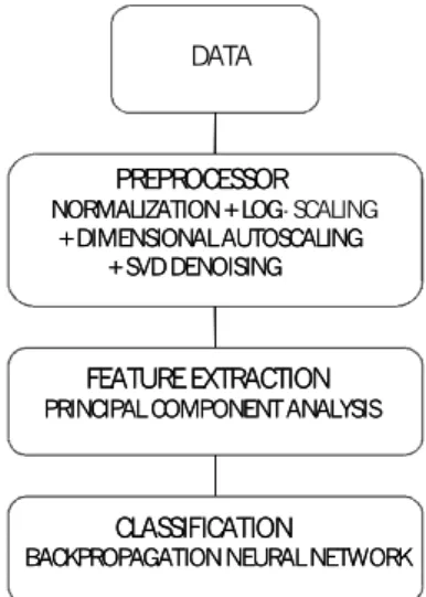
A pattern-recognition system consists of preprocessor, feature extraction, and classification stages. In each stage, several processing sub-steps are used, either independently or in combination. The goal of a pattern-recognition system is to optimise classification efficiency through proper selection of methods at each stage, and by establishing the best Data generated* from the model SAW sensor array for TNT detection
Vapours Concen-tration Sensor 1 FPOL Sensor 2 PDMS Sensor 3 PIB Sensor 4 PECH Sensor 5 PVPR Sensor 6 PEI Sensor 7 SXCN Sensor 8 PVTD Sensor 9 ZDOL Sensor 10 OV202 Sensor 11 PMPS TNT 1 ppt -101.02 5.531 179.78 -116.11 -119.71 -281.13 -153.09 -153.09 -41.361 26.491 132.7 TNT 2 ppt -141.5 57.296 -132.88 -450.55 -190.81 -243.99 86.699 149.04 -94.107 -77.366 -115.89 TNT 3 ppt 9.1783 -199.84 -122.47 -482.79 -482.79 -657.48 -657.48 34.213 -176.09 184.4 -40.206 TNT 4 ppt -151.97 -151.97 170.94 -719 -719 -1023.2 -83.649 -173.16 -177.71 -57.959 95.739 TNT 5 ppt -274.72 -141.42 -64.686 -64.686 -173.28 -1036.7 -310.17 -21.14 42.224 130.2 22.794 DNT 1 ppt 123.98 -149.48 131.76 -122.44 -97.711 143 -108.15 68.479 -156.66 -146.33 -135.38 DNT 2 ppt -123.45 104.84 46.552 -68.36 -7.0499 -134.43 50.84 -67.571 24.962 24.962 123.16 DNT 3 ppt -172.83 168.95 -24.065 -193.39 48.882 -149.85 -210.7 -160.93 43.087 169.27 -156.58 DNT 4 ppt -26.228 198.65 -129.23 -176.81 42.625 -9.1975 -9.4413 -148.94 -148.94 -148.94 39.406 DNT 5 ppt -16.608 36.026 -115.09 -100.14 56.331 -210.53 120.24 -59.206 177.59 177.59 52.262 TOL 1 ppm -0.6335 -87.198 52.542 52.542 178.05 178.05 178.05 139.59 69.878 70.06 70.06 TOL 2 ppm -198.18 -136.2 -136.2 69.97 24.334 -74.152 -74.152 -74.152 147.19 43.549 -59.632 TOL 3 ppm 146.21 146.21 -209.57 1.7774 1.7774 -112.27 -112.27 9.0389 9.0389 -79.156 -7.2819 TOL 4 ppm -47.478 -179.31 -38.311 -25.368 -25.368 42.766 -131.16 -172.27 -27.842 -5.2981 -5.2981 TOL 5 ppm 141.56 141.56 34.689 111.49 107.29 34.597 44.002 44.002 101.6 5.8881 -31.43 BNZ 1 ppm -289.52 -5.3536 136.75 38.043 -38.453 -74.867 210.26 -14.828 27.376 27.376 53.684 BNZ 2 ppm 53.684 53.684 -153.52 -153.52 -153.52 -153.52 -153.52 -151.35 92.194 92.194 148.75 BNZ 3 ppm 190.97 -22.338 -160.78 16.215 32.555 -110.81 85.905 43.066 85.433 40.027 -33.783 BNZ 4 ppm -33.783 -161.91 -161.91 -17.247 -56.84 -212.18 -102.69 146.35 146.35 161.31 -85.912 BNZ 5 ppm 185.74 182.37 182.37 182.37 66.814 66.814 66.814 66.814 42.654 -101.56 201.94 DMMP 1 ppb -65.836 142.7 142.7 22.77 25.64 25.64 84.272 84.272 45.414 137.27 -8.0665 DMMP 2 ppb 162.37 -20.791 173.99 3.8917 41.557 -11.303 -23.42 167.27 -8.6975 179.82 119.19 DMMP 3 ppb -28.468 111.33 111.33 161.25 161.25 -112.95 13.911 79.721 -78.907 182.86 104.75 DMMP 4 ppb -44.228 176.32 176.32 176.32 176.32 81.668 -109.04 -61.462 -77.645 -23.315 31.816 DMMP 5 ppb 31.816 31.816 94.387 94.387 18.469 -195.62 -114.48 104.46 155.4 155.4 155.4 H2O 10 ppb -117.66 -117.66 38.042 -75.565 -187.88 5.2368 -18.618 -166.71 -73.088 -154.36 -103.35 H2O 20 ppb -103.35 162.84 -107.7 -107.7 161.11 -67.276 -59.345 -12.097 -181.22 -110.69 65.718 H2O 30 ppb -155.71 92.281 165.39 -180.15 -180.15 47.093 69.44 -154.98 92.084 217.09 -79.017 H2O 40 ppb 206 206 -72.335 -153.1 117.37 117.37 -76.6 136.76 73.915 -39.372 -92.899 H2O 50 ppb 91.2 -174.73 103.28 -109.99 -1.2393 -320.82 -196.18 -196.18 -196.18 -196.18 182.85
Table 4. Synthetic data matrix generated by the model SAW sensor array for 5 concentrations of each vapour
*Note: The data includes a Gaussian noise source with random mean over [30,+30] Hz and fixed standard deviation 10 Hz, and random outliers with uniform distribution over [50,+50] Hz
among several alternate combinatorial possibilities. Often, different combination strategies work best in different application domains. In SAW sensor array-based vapour recognition system, it has been found recently41-43 that a preprocessor comprised data normalisation wrt polymer thickness and vapour concentration, then logarithmic scaling followed by denoising by singular value decomposition (SVD) in combination with the principal component analysis (PCA) for feature extraction and the neural network classification yields substantially enhanced classification rate. The validation data used in these analyses were collected from the published literature, and pertained to the sensing of a number of volatile organic compounds including nerve agents and environmental hazards. In the present work which proposes simulated SAW sensor array model as a validation tool for pattern recognition algorithms, the same preprocessing and pattern recognition strategy has been adopted. It is shown schematically in Fig. 1. The method is summarised as follows.
The data was, first prepared by dividing the output of each sensor Dfij by the respective vapour concentrations
C i and frequency shifts j p
f
D due to polymer coatings, and then taking their logarithms to define new data matrix as
log( i j)
ij ij p
f f C f
D ¬ D D . Next, the data matrix was mean-centered and variance-normalised wrt the vapour samples for each sensor in the array. This is called dimensional autoscaling44, and it is implemented as ( ) /
ij ij j j f f f D ¬ D - D s where 1 (1/ )N ij ij i f N f = D =
å
D and 2 1 (1 / ) (N ) j ij j i N f f = s =å
D - Drepresents the column mean and standard deviation, respectively. Then, the denoising was done by truncating the full rank SVD expansion of the redefined data matrix by a matrix of lower rank. The procedure implicitly assumes that the rank of the data matrix is lower than the number
of sensors in the array. The details of SVD denoising are presented43. The data matrix regenerated on the basis of truncated SVD approximates the original data with reduced noise.The preprocessed data matrix as explained above is then PCA processed, and the first few principal components are taken to define the set of features to represent vapour identities. The classification is done by artificial neural network based on the training by error backpropagation algorithm.
4.1 Implementation
The synthetic data generation was done by the method described in Section 3. The preprocessing, denoising by SVD, and feature extraction by PCA were done as described in the preceding. For classification, the four commonly used classifiers in electronic nose data analysis were used with an aim to examine their relative performance under noisy conditions. These were: artificial neural network with error backpropagation algorithm (ANN), K-nearest neighbour (KNN), naïve Bayes, and support vector machine (SVM). Most of the programs were implemented in MATLAB environment. However, the KNN, naïve Bayes, and SVM classifiers were implemented in R. The classifiers were trained with total 120 samples taken to represent 20 samples from each of the 6 classes (TNT, DNT, toluene, benzene, DMMP and water), and tested with 60 samples (10 samples from each class).
The 180´11 data matrix created by the 11 sensors array were preprocessed with and without SVD denoising. This was followed by PCA-based feature extraction and classification. The classification was done using only 3 highest eigenvalue principal components. The ANN was implemented using a 3-layer architecture (3´6´6) with 3 neurons in the input layer, 6 neurons in the hidden layer, and 6 neurons in the output layer. The trainbfg function with tansig activation in the hidden layer and linear activation in the out-layer were used with the training goal set at 105. The convergence was achieved typically after 300 epochs. The KNN was implemented using class package45 in R with k = 5. The naïve Bayes and SVM classifiers were implemented using e1071 package46 in R. The value the tuning parameter Laplace for naïve Bayes was set to be zero. This resulted in best results. For SVM, the radial Gaussian kernel with tuning parameter gamma = 0.5 produced the best results.
5. VALIDATION RESULTS
5.1 Preprocessing and Principal Component Analysis Scores
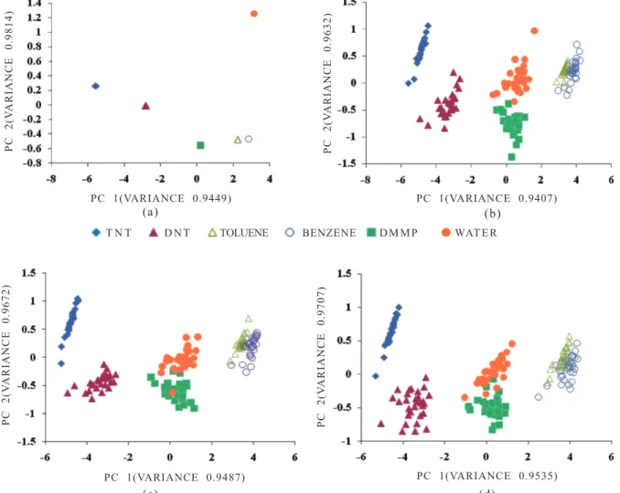
Figure 2 through Fig. 5 show PCA results of the whole 180 ´ 11 data matrix generated under different noise and processing conditions. In Fig. 2 are shown the results with 4 levels of noise strength without doing SVD denoising. This shows how the presence of noise sources in data acquisition makes blurs class separability in feature space. When no noise is added, all the points of a class coincide, and different classes are distinctly separated, Fig. 2(a).
CLASSIFICATION
BACKPROPAGATION NEURAL NETWORK
FEATURE EXTRACTION
PRINCIPAL COMPONENT ANALYSIS
PREPROCESSOR
NORMALIZATION + LOG SCALING + DIMENSIONAL AUTOSCALING
+ SVD DENOISING
DATA
CLASSIFICATION
BACKPROPAGATION NEURAL NETWORK
FEATURE EXTRACTION
PRINCIPAL COMPONENT ANALYSIS
PREPROCESSOR
NORMALIZATION + LOG-+ DIMENSIONAL AUTOSCALING
+ SVD DENOISING
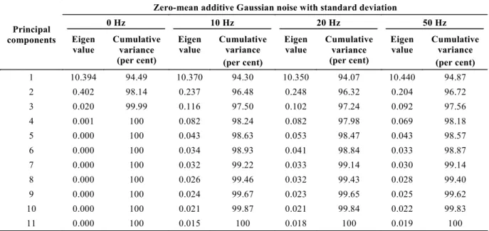
As the magnitude of noise increases, the sample points of each class get scattered and neighbouring classes begin to overlap, Figs 2(b) to (d). This makes the task of classification difficult; particularly note the mixing of toluene and benzene samples, and DMMP and water samples. The level of difficulty goes up in proportion to the magnitude of noise. This shows how vital it is to employ an appropriate data denoising method in the preprocessor stage. Table 5 shows the eigenvalues and cumulative variances of principal components. Notice that without noise, the complete information (measured by cumulative variance) is contained in the first 3 principal components. With noise added, a small part of information (< 3 per cent) is spread over 8 principal components. If one eliminates these 8 principal components to reduce the dimensionality of problem, some information is lost, and is not available to the classifier. Often, one has to trade-off the impact of this loss on the classifier performance and the computational gain in terms of reduced dimensionality. Figure 3 shows the importance of data cleaning by SVD denoising prior to doing PCA. It can be noticed that both intraclass and interclass dispersion is reduced after denoising; particularly notice the compaction
of TNT sample points and separability of toluene and benzene samples.
Two more types of difficulty levels were added to the synthetic data to examine the influence of SVD denoising on feature extraction. In one case, the mean output of the noise source was randomly varied assuming a uniform distribution over a certain range of values keeping the standard deviation fixed. In the other case, outliers were further added to this noise source. To add the outliers, a random outlier value was generated within a range assuming uniform distribution along with a probability value using a normal distribution function. If the probability value exceeds a certain predefined threshold (say, 0.9) then that outlier was added to the noise source output. Figure 4 and 5 show the PCA results after the first and the second type of data corruption, respectively. In the first case, mean value was generated over [-30, +30] Hz keeping the standard deviation 10 Hz. In the second case, the outliers were added over [-50, +50] Hz. Recall that the fundamental frequency of operation of SAW oscillators has been taken to be 200 MHz. The data corruption in the Hz range therefore implies ppm (parts per million) level of SAW oscillator T N T D N T TOLUENE BENZENE D M M P WATER
PC 1(VARIANCE 0.9449) PC 1(VARIANCE 0.9535) PC 1(VARIANCE 0.9487) PC 1(VARIANCE 0.9407) PC 2(V ARIANCE 0.9814) PC 2(V ARIANCE 0.9707) PC 2(V ARIANCE 0.9672) PC 2(V ARIANCE 0.9632)
Figure 2. Principal component score plots of the model sensor array response for different levels of additive Gaussian noise. (a) No noise (noise source with zero mean and zero standard deviation), (b) noise with zero mean and 20 Hz standard deviation, (c) noise with zero and 50 Hz standard deviation, and (d) noise with zero mean and 100 Hz standard deviation.
(a) (b)
PC 1(VARIANCE 0.9297)
PC 2(V
ARIANCE 0.9597)
TNT DNT TOLUENE BENZENE DMMP WATER
PC 1(VARIANCE 0.9430)
PC 2(V
ARIANCE 0.9648)
Zero-mean additive Gaussian noise with standard deviation
0 Hz 10 Hz 20 Hz 50 Hz
Principal
components Eigen
value Cumulative variance (per cent)
Eigen
value Cumulative variance (per cent)
Eigen
value Cumulative variance (per cent)
Eigen
value Cumulative variance (per cent) 1 10.394 94.49 10.370 94.30 10.350 94.07 10.440 94.87 2 0.402 98.14 0.237 96.48 0.248 96.32 0.204 96.72 3 0.020 99.99 0.116 97.50 0.102 97.24 0.092 97.56 4 0.001 100 0.082 98.24 0.082 97.98 0.069 98.18 5 0.000 100 0.043 98.63 0.053 98.47 0.043 98.57 6 0.000 100 0.034 98.93 0.041 98.84 0.033 98.87 7 0.000 100 0.032 99.22 0.033 99.14 0.030 99.14 8 0.000 100 0.026 99.46 0.032 99.43 0.028 99.40 9 0.000 100 0.024 99.67 0.023 99.65 0.025 99.62 10 0.000 100 0.021 99.87 0.021 99.84 0.022 99.83 11 0.000 100 0.015 100 0.018 100 0.019 100 PC 1(VARIANCE 0.9283) PC 2(V ARIANCE 0.9508)
TNT DNT TOLUENE BENZENE DMMP WATER
PC 1(VARIANCE 0.9564)
PC 2(V
ARIANCE 0.9735)
Figure 3. Principal component score plots of the model sensor array response corrupted with zero-mean 10 Hz standard deviation Gaussian noise source: (a) without denoising, and (b) after SVD denoising.
Figure 4. Principal component score plots of the model SAW sensor array response with data corrupted by a noise source having random mean over [-30, + 30] Hz and standard deviation 10 Hz: (a) without denoising, and (b) after denoising.
Table 5. Eigenvalues of principal components and cumulative variances of the model sensor array data corrupted with noise sources of different strengths
(a)
(b)
(a)
stabilities. This is quite realistic for the SAW sensors. The influence of SVD denoising is clearly evident in Fig. 4. The separation between classes improves, and within a class the sample points are more compactly represented after denoising. Table 6 summarises the eigenvalues and cumulative variance results for this data. From a comparison of the trends of cumulative variances, it can be seen that the SVD spreads some information to higher principal components which will be lost during truncation for denoising. However, as will be seen from the classification results in Table 8, this loss is upset by the gain due to improved interclass separation.
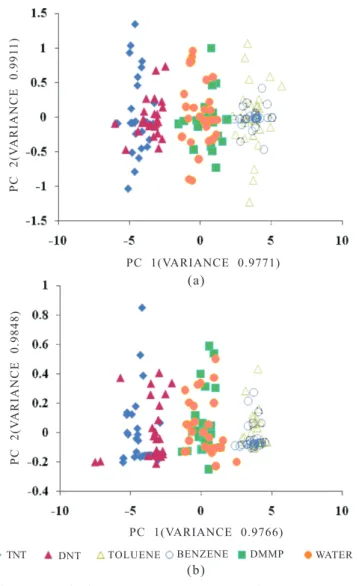
The effect of adding outliers is however highly detrimental. This can be seen from the principal component score plots in Fig. 5. The overlaps between different classes have increased to such a level that it is nearly impossible to discriminate between TNT and DNT, between DMMP and water, and between toluene and benzene samples. If the data points in these pairs can be taken together to
represent a single class, then the analysis can, at the most, discriminate samples among 3 classes. It can also be noted that the effect of SVD denoising in this case is only marginal. It underlines the non-usability of SVD expansion and truncation in outlier detection and rejection. Table 7 summarises the PCA eigenvalue and cumulative variance results for this case. The variance distribution is not affected much by SVD denoising.
PC 1(VARIANCE 0.9766) PC 2(V ARIANCE 0.9848) PC 1(VARIANCE 0.9771) PC 2(V ARIANCE 0.991 1)
TNT DNT TOLUENE BENZENE DMMP WATER Figure 5. Principal component score plots of the model sensor
array response with data corrupted by Gaussian additive noise as in Fig. 3 and the random outliers having magnitudes over [50, +50] Hz: (a) without SVD denoising, and (b) after SVD denoising.
Data corrupted with Gaussian additive noise with random mean over [-30, +30] Hz and standard deviation fixed at 10 Hz
Without SVD denoising After SVD denoising Principal component Eigen value Cumulative variance (per cent) Eigen value Cumulative variance (per cent) 1 10.521 95.65 10.021 92.83 2 0.1907 97.38 0.2483 95.08 3 0.0585 97.91 0.1495 96.44 4 0.0475 98.34 0.0912 97.27 5 0.0395 98.70 0.0867 98.06 6 0.0313 98.98 0.0623 98.63 7 0.0279 99.24 0.0501 99.08 8 0.0264 99.48 0.0372 99.42 9 0.0237 99.69 0.0317 99.71 10 0.0184 99.86 0.2076 99.90 11 0.0152 100 0.0113 100 Table 6. Influence of SVD denoising on PCA results
(a)
(b)
Data corrupted with Gaussian additive noise with random mean over [-30, +30] Hz and standard deviation fixed at 10 Hz, and outliers over [-50, +50] with probability threshold 0.9
Without SVD
denoising After SVD denoising Principal component Eigen value Cumulative variance
(per cent) Eigen value
Cumulative variance (per cent) 1 10.748 97.71 10.743 97.66 2 0.1593 99.91 0.0897 98.48 3 0.0429 99.50 0.0560 98.98 4 0.0201 99.68 0.0366 99.31 5 0.0116 99.79 0.0249 99.55 6 0.0069 99.85 0.0183 99.71 7 0.0056 99.90 0.0129 99.82 8 0.0038 99.93 0.0079 99.90 9 0.0033 99.96 0.0061 99.95 10 0.0026 99.99 0.0038 99.98 11 0.0009 100 0.0015 100 Table 7. Influence of SVD denoising on PCA results of data
5.2 Classification
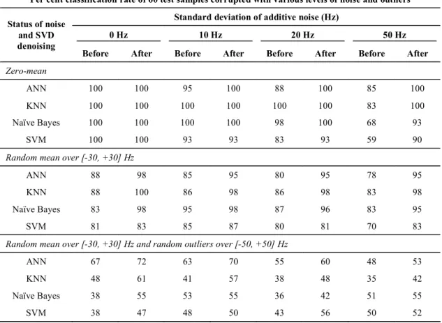
Table 8 summarises the classification results obtained using four classifiersbackpropagation artificial neural network (ANN), K-nearest neighbour (KNN), Naïve Bayes, and support vector machine (SVM). The data with zero noise yields 100 per cent correct classification as expected. As the noise level increases, the classification rate decreases, being the worst in case of noise added with outliers. It can be noted that in general, the SVD denoising improves the classification rate significantly with all the classifiers. These results also reveal some interesting aspects of different classifiers. One particularly noticeable feature is the performance the ANN classifier. This remains perhaps the most robust in the presence of challenges due to additive Gaussian noise and outliers. The ANN consistently produces high result. In comparison, the KNN and Naïve Bayes yield competing and sometimes better performance if the outliers are not present. However, by addition of outliers their performance (particularly KNN) deteriorates dramatically. The SVM does not yield as high results in the case of noisy data, though it seems to do better in the presence of high noise and outliers. The SVM appears to be more suited for outlier detection in noisy data. Table 9 shows the confusion matrix for one analysis. It can be seen from this table that maximum confusion occurs between class 3 and class 4 which are toluene and benzene respectively, (Table 3). It is consistent with the PCA score plots shown in Fig. 2 through Fig. 4. The toluene and
benzene separation is lowest in feature space. The influence of outliers in destroying class separability is quite apparent in Fig. 5.
6. CONCLUSIONS
The synthetic data generated by SAW sensor array simulation is found to be quite useful in experimenting with pattern recognition methods. The sensor array model can be extended to include any number of polymers, and some other physical phenomena such as drift, aging, thermal noise, flicker noise, and response non-linearity through their proper mathematical representation. This type of synthetic data provides two types of advantages. One, an optimum set of polymers can be selected to impart the largest class separation in the feature space without actually doing experiments with the real material and sensors. The latter is quite cost intensive and time-consuming exercise. Second, the anticipated disturbances in the sensor operation or data acquisition can be modeled and incorporated in the array response. This can then be used either to test efficacy of the existing pattern recognition procedures or to develop new methods to obtain better classification accuracy. The development of pattern recognition system is perhaps the most costly component in the development of an electronic nose system. Therefore, this approach to search for the appropriate sensors and to optimise data processing procedures will be of great help in reducing the time and cost of electronic nose development. Though the case study presented
Per cent classification rate of 60 test samples corrupted with various levels of noise and outliers Standard deviation of additive noise (Hz)
0 Hz 10 Hz 20 Hz 50 Hz
Status of noise and SVD denoising
Before After Before After Before After Before After Zero-mean
ANN 100 100 95 100 88 100 85 100 KNN 100 100 100 100 100 100 83 100
Naïve Bayes 100 100 100 100 98 100 68 93
SVM 100 100 93 93 83 93 59 90 Random mean over [-30, +30] Hz
ANN 88 98 85 95 80 95 78 95 KNN 88 100 86 98 86 98 83 98
Naïve Bayes 83 98 95 98 87 96 83 95
SVM 81 83 85 87 80 81 70 83 Random mean over [-30, +30] Hz and random outliers over [-50, +50] Hz
ANN 67 72 63 70 55 60 48 53 KNN 48 61 41 57 38 48 35 42
Naïve Bayes 38 55 53 55 36 42 51 55
SVM 38 47 48 50 43 56 50 52 Table 8. Effect of noise and outlier on classification using ANN, KNN, Naïve Bayes, and SVM classifiers
here implements only a limited set of possibilities, the analysis clearly underlines the usefulness of this strategy. As example, the role of singular value decomposition in denoising the sensor array data and its impact on the classification accuracy is illustrated, the role of outliers and the difficulty they create in pattern recognition is demonstrated, and the relative effectiveness of different classifiers under varied noise is analysed.
ACKNOWLEDGEMENTS
This work was supported in part by the Defence Research & Development Organisation (Government of India) under Grant ERIP-ER-0703643-01-1025 and by Department of Science and Technology (Government of India) under Grant DST-TSG-PT-2007-06. The author Shri S.K. Jha is thankful to the Directorate of Forensic Science, Ministry of Home Affairs, New Delhi and the Director, Central Forensic Science Laboratory, Chandigarh, for their support and JRF sponsorship. The authors are thankful to their colleagues Mr Prashant Singh, Mr Shashank S. Jha, Ms Divya Somvanshi and Mr Dinesh Kumar for their support and cooperation. REFERENCES
1. Singh, Suman. Sensorsan effective approach for the detection of explosives. J. Hazard. Mater., 2007, 144, 15-28.
2. Dionne, B.C.; Rounbehler, D.P.; Achter, E.K.; Hobbs,
J.R. & Fine, D.H. Vapour pressure of explosives. J. Energetic Mater., 1986, 4(1), 447-72.
3. Review of conventional electronic noses and their possible application to the detection of explosives. In Electronic noses and sensors for the detection of explosives, edited by J.W. Gardner & Kluwer, J. Yinon. Ch. 1. 2004.
4. Yinon, J. Detection of explosives by electronic noses. Analytical Chemistry, 2003, 75(5), 99A-105A. 5. Pamula, V.K. Detection of explosives. In Handbook
of machine olfaction: Electronic nose technology, edited by T.C. Pearce, S.S. Schiffman, H.T. Nagle & J.W. Gardner. Willy-VHC Verlag GmbH & Co., Weinheim, 2003. pp. 547-60.
6. Settles, G.S. & Kester D.A. Aerodynamic sampling for landmine trace detection. SPIE Aerosense, April 2001, Vol. 4394. Paper No. 108.
7. Wilson, A.D. & Baietto, M. Applications and advances in electronic nose technologies. Sensors, 2009, 9, 5099-148.
8. Sarah, J. T. & William, C.T. Polymer sensors for nitroaromatic explosives detection. J. Mater. Chem., 2006, 16, 2871-883.
9. James, D.; Simon, M.S.; Zulfiqur, A. & OHare, W.T. Chemical sensors for electronic nose systems. Microchimica Acta, 2005, 149, 1-17.
10. Hughes, R.C.; Ricco, A.J.; Butler, M.A. & Martin, S.J.
ANN KNN
Predicted class rate (per cent) Classification Predicted class rate (per cent) Classification
9 2 0 0 0 0 9 2 0 0 0 0 1 8 0 0 0 0 1 8 0 0 0 0 0 0 8 5 0 0 0 0 8 1 1 0 0 0 2 5 0 0 0 0 2 9 2 0 0 0 0 0 9 2 0 0 0 0 7 1 True class 0 0 0 0 1 8 78 True class 0 0 0 0 0 9 83 SVM Naïve Bayes
Predicted class rate (per cent) Classification Predicted class rate (per cent) Classification
5 4 0 0 0 0 6 0 0 0 0 0 5 6 0 0 0 0 4 10 0 0 0 0 0 0 10 6 0 0 0 0 8 0 0 0 0 0 0 4 0 0 0 0 2 10 0 0 0 0 0 0 8 1 0 0 0 0 8 2 True class 0 0 0 0 2 9 70 True class 0 0 0 0 2 8 83 Table 9. Confusion matrix for ANN, KNN, Naïve Bayes, and SVM classifiers in the analysis
of noisy data corrupted with additive Gaussian noise source random mean over [-30, +30] Hz and standard deviation 50 Hz
Chemical microsensors. Science, 1991, 254(5028), 74-80.
11. Murray, M.G. & Southard, G.E. Sensors for chemical weapons detection. IEEE Instrum. Meas. Magazine, 2002, 5(4), 12-21.
12. Dorozhkin, L.M. & Rozanov, I.A. Acoustic wave chemical sensors for gases. Analytical Chemistry, 2001, 56 (5), 399-16.
13. Dickert, F.L.; Forth, P.; Bulst, W.E.; Fischerauer, G. & Knauer, U. SAW devices-sensitivity enhancement in going from 80 MHz to 1 GHz. Sensors Actuators B, 1998, 46, 120-25.
14. Yadava, R.D.S. Enhancing mass sensitivity of SAW delay line sensors by chirping transducers. Sensors Actuators B, 2006, 114, 127-31.
15. Yadava, R. D. S.; Kshetrimayum, R. & Khaneja, Mamta. Multifrequency characterization of viscoelastic polymers and vapour sensing based on SAW oscillators. Ultrasonics, 49(8), 638-45.
16. Kshetrimayum, R.; Yadava, R.D.S. & Tandon, R.P. Mass sensitivity analysis and designing of surface acoustic wave resonators for chemical sensors. Meas. Sci. Technol., 2009, 20, 1-10.
17. Malocha, D.C.; Pavlina, J.; Gallagher, D.; Kozlovski, N.; Fisher, B.; Saldanha N. & Puccio, D. Orthogonal frequency coded SAW sensors and RFID design principles. In IEEE Frequency Control Symposium, May 2008. pp. 278-83.
18. Grate, J.W. Acoustic wave microsensor arrays for vapour sensing. Chemical Review, 2000, 100, 2627-648. 19. Microsensors and sensor microsystems - SAW arrays/
integrated-SAW. http://www. sandia.gov/mstc/ MsensorSensorMsystems/technical-information/. 20. Sherrit, S.; Bao, X.Q.; Bar-Cohen, Y. & Chang, Z.
BAW and SAW sensors for in-situ analysis. In Proceedings SPIE Smart Structures Conference, San Diego, CA., 2-6 Mar, 2003, Vol. 5050, Paper No.11. 21. Alizadeh, T., Zeynali, S. Electronic nose based on the polymer coated SAW sensors array for the warfare agent simulants classification. Sensors Actuators B, 2008, 129, 412-23.
22. Staples, E.J. & Viswanathan, S. Development of a novel odour measurement system using gas chromatography with surface acoustic wave sensor. J. Air Waste Manag. Asso., 2008, 58(12), 1522-528. 23. Reibel, J.; Stahl, U.; Wessa, T. & Rapp, M. Gas analysis with SAW sensor systems. Sensors Actuators B, 2000, 65, 173-75.
24. Moore, D.S. Instrumentation for trace detection of high explosives. Rev. Sci. Instrum., 2004, 75(8), 2499-512.
25. Skrypnik, A.; Voigt, A. & Rapp, M. in-situ soil gas analysis with a robust SAW sensor system integrated in percussion driven penetration cones. In IEEE Transducers Conf. (Solid-State Sensors, Actuators and Microsystems), June 2007. pp. 1007-10. 26. Crtsalnuovo, S.A.; Frye-Mason, G.C.; Kottenstette,
R. J.; Heller, E. J.; Matzke, C. M.; Lewis, P.R.; Manginell,
R.P.; Baca, A.G.; Hletala, V.M. & Wendt, J.R. Gas phase chemical detection with an integrated chemical analysis system, Sandia National Laboratories Report No. SAND2000-0250C. Apr 2000.
27. Zellers, E.T.; Batterman, S.A.; Han, M. & Patrash, S. J. Optimal coating selection for the analysis of organic vapour mixtures with polymer-coated surface acoustic wave sensor arrays. Analytical Chemistry, 1995, 67(6), 1092-106.
28. Ho, C.K.; Lindgren, E.R.; Rawlinson, K.S.; McGrath. L.K. & Wright, J.L. Development of a surface acoustic wave sensor for in-situ monitoring of volatile organic compounds. Sensors, 2003, 3, 236-47.
29. McGill, R.A.; Mlsna, T.E.; Chung, R; Nguyen, V.K. & Stepnowski, J. The design of functionalised silicon polymers for chemical sensor detection of nitroaromatic compounds. Sensors Actuator B., 2000, 65(1-3), 5-9. 30. Gardner, J.W.; Boilot, P. & Hines, E.L. Enhancing electronic nose performance by sensor selection using a new integer-based genetic algorithm approach, Sensors Actuators B., 2005, 106, pp. 114-121.
31. Corcoran, P.; Anglesea, J. & Elshaw, M. The application of genetic algorithms to sensor parameter selection for multisensor array configuration. Sensors Actuators, 1999, 76, 57-66.
32. Nishikawa, T.; Hayashi, T.; Nambo, H.; Kimura, H. & Oyabu, T. Feature extraction of multi-gas sensor responses using genetic algorithm. Sensors Actuators B, 2000, 64, 2-7.
33. Hierlemann, A.; Ricco, A. J.; Bodenhofer, K. & Gopel, W. Effective use of molecular recognition in gas sensing: results from acoustic wave and in-situ FTIR measurements, Analytical Chemistry, 1999, 71, 3022-035.
34. Hoang, S.H.; Horng, G.D.; Chiang, C.Y., Ko, C.H.; Lo, Y.C.; Chen, C. I. & Chang, C.K. A novel measurement Device for SAW Chemical Sensors with FT-IR Spectro-microscopic Analytical Capability, Tamkang J. Sci. Eng., 2004, 7(2), 99-102.
35. Albert, K.J.; Lewis, N.S.; Schauer, C.L.; Sotzing, G..A.; Stitzel, S.E.; Vaid, T. P.& Walt, D.R.Cross-Reactive Chemical Sensor Arrays. Chemical Review, 2000, 100, 2595-626.
36. Park, J.; Groves, W. A. & Zellers, E. T. Vapour recognition with small arrays of polymer-coated microsensors a comprehensive analysis. Analytical Chemistry, 1999, 71, 3877-886.
37. Martin, S.J.; Frye, G.C. & Senturia, S.D. Dynamics and response of polymer-coated surface acoustic wave devices: effect of viscoelastic properties and film resonance. Analytical Chemistry, 1994, 66(14), 2201-219. 38. Rebiere, D.; Dejous, C.; Pistre, J.; Planade, R.; Lipskier,
J. & Robin, P. Surface acoustic wave detection of organophosphorus compounds with fluoropolyol coatings. Sensors Actuator B, 1997, 43, 34-39. 39. Houser, E.J.; Mlsna, T.E.; Nguyen, V.K.; Chung, R;
Mowery, R.L. & McGill, R.A. Rational materials design of sorbent coatings for explosives: applications with chemical sensors. Talanta, 2001, 54(3), 469-84.
40. Rebiere, D.; Dejous, C.; Pistre, J.; Planade, R.; Lipskier, J. & Robin, P. Surface acoustic wave detection of organophosphorus compounds with fluoropolyol
coatings. Sensors Actuator B., 1997, 43, 34-39.
41. Yadava, R.D.S. & Chaudhary, Ruchi. Solvation, transduction and independent component analysis for pattern recognition in SAW electronic nose. Sensors Actuators B, 2006, 113, 1-21.
42. Jha, S.K. & Yadava, R.D.S. Preprocessing of SAW sensor array data and pattern recognition. IEEE Sensors J., 2009, 9(10), 1202-208.
43. Jha, S.K. & Yadava, R.D.S. Denoising by singular value decomposition and its application to electronic nose data processing. IEEE Sensors J. (in press). 44. Osuna, R.G. & Nagle, H.T. A method for evaluating
data preprocessing techniques for odour classification
with an array of gas sensors, IEEE Trans. Syst. Man
Cybern. B., 1999, 29(5), 626-32.
45. Venables, W.N. & Ripley, B.D. Modern applied statistics with S. Ed. 4. Springer, New York, 2002.
46. Dimitriadou, E., Hornik, K., Leisch, F., Meyer, D. & Weingessel, A. Misc functions of the Department of Statistics (e1071), TU Wien. R package Ver 1. 2008, 5-18.
47. Harper, Ross J.; Almirall, José R. & Furton, Kenneth G. Identification of dominant odor chemicals emanating from explosives for use in developing optimal training aid combinations and mimics for canine detection.
Talanta, 2005, 67(2), 313-27.
48. Tevault, D. E.; Buchanan, J. H. & Buettner, L. C. Ambient
Contributors
Mr S.K. Jha obtained his BSc and MSc in Physics from Udai Pratap Autonomous College, Varanasi, affiliated to V.B.S. Purvanchal University, Jaunpur, India, in 2003 and 2005, respectively. He is Junior Research Fellow sponsored by the Central Forensic Science Laboratory, Chandigarh, and is pursuing PhD at the Department of Physics, Banaras Hindu University, Varanasi. His research interests include: sensor array vapour detection of illicit materials, signal processing, multivariate data processing, and pattern recognition.
Dr R.D.S. Yadava received his PhD (Physics) from Banaras Hindu University, Varanasi, in 1981. He is presently a Professor of Physics in the Department of Physics, Faculty of Science, Banaras Hindu University, Varanasi. His current research interests include: sensor array systems, signal processing, electronic nose, pattern recognition, sensor/data fusion based on acoustic wave (SAW and QCM), conducting polymer, metal-oxide and cantilever sensor technologies.
volatility of DMMP. Int. J. Thermophysics. 2006, 27(2), 486-93.
49. CRC handbook of chemistry and physics, Edited by