SEASONED EQUITY OFFERINGS AND MARKET VOLATILITY
by
CHANYOUNG EOM
A DISSERTATION
Presented to the Department of Finance and the Graduate School of the University of Oregon
in partial fulfillment of the requirements for the degree of
Doctor of Philosophy June 2011
DISSERTATION APPROVAL PAGE Student: Chanyoung Eom
Title: Seasoned Equity Offerings and Market Volatility
This dissertation has been accepted and approved in partial fulfillment of the requirements for the Doctor of Philosophy degree in the Department of Finance by:
Dr. Roberto Gutierrez Chair
Dr. Ekkehart Boehmer Member
Dr. Wayne Mikkelson Member
Dr. Jeremy Piger Outside Member
and
Richard Linton Vice President for Research and Graduate Studies/Dean of the Graduate School
Original approval signatures are on file with the University of Oregon Graduate School. Degree awarded June 2011
c
DISSERTATION ABSTRACT Chanyoung Eom
Doctor of Philosophy Department of Finance June 2011
Title: Seasoned Equity Offerings and Market Volatility Approved:
Dr. Roberto Gutierrez
New equity shares are sold for raising capital via a primary seasoned equity offering (SEO). In their 2010 article, Murray Carlson, Adlai Fisher, and Ron Giammarino discovered an intriguing relationship between market volatility and primary SEOs, namely that the volatility decreases before a primary SEO and increases thereafter. This pattern contradicts the real options theory of equity issuance for investment. In this study, I examine in greater detail whether the pre- and post-issue volatility dynamics are related to the probability of issuing new equity. I find little evidence that the decision to conduct a primary SEO depends on changes in market volatility after controlling for previously recognized determinants of SEOs. This reconciles the volatility finding of Carlson et al. with the real options theory of equity issuance for investment. I also examine secondary SEOs, in which only existing equity shares are sold and therefore no capital is raised by the firm. For secondary SEOs, real options theory makes no predictions about risk changes around the events. I find that market volatility tends to decline before a secondary SEO, a finding which warrants further attention.
CURRICULUM VITAE
NAME OF AUTHOR: Chanyoung Eom
GRADUATE AND UNDERGRADUATE SCHOOLS ATTENDED: University of Oregon, Eugene, Oregon
University of Cincinnati, Cincinnati, Ohio University of Iowa, Iowa City, Iowa Hanyang University, Seoul, South Korea DEGREES AWARDED:
Doctor of Philosophy in Finance, 2011, University of Oregon Master of Science in Finance, 2006, University of Cincinnati Master of Science in Statistics, 2005, University of Iowa Bachelor of Arts in Economics, 2001, Hanyang University
ACKNOWLEDGEMENTS
I gratefully acknowledge beneficial comments from Ekkehart Boehmer, Roberto Gutierrez (chair), Wayne Mikkelson, and Jeremy Piger. Special thanks go to Roberto Gutierrez for helpful discussion and numerous comments which have significantly improved this paper. I also thank Diane Del Guercio for useful comments. Finally, I thank Egemen Genc for providing the data of quarterly liquidity. All remaining errors are mine.
This dissertation is dedicated to my wife, Hyunjae, and children, Yumin and Taeil, who have always given me a smile and believed that I could do it.
TABLE OF CONTENTS
Chapter Page
I. INTRODUCTION . . . 1
II. DATA . . . 4
III. EXTENSION OF CARLSON ET AL. (2010) . . . 9
IV. VOLATILITY TIMING . . . 15
4.1. Test Specification . . . 15
4.2. Stationary Test . . . 18
4.3. Empirical Proxies . . . 20
4.4. Empirical Results . . . 29
V. CONCLUSION . . . 43
APPENDIX: DERIVATION OF EQUATION 4.2. . . 45
LIST OF FIGURES
Figure Page
3.1. Event-time EW Averages of Market Volatility . . . 11 4.1. SEO Volume and Other Empirical Proxies over 1Q 1970 – 4Q 2005 . . . 26 4.2. Orthogonalized Impulse Response Functions (IRFs) . . . 32
LIST OF TABLES
Table Page
2.1. Summary Statistics and Jensen’s Alphas . . . 5
2.2. Frequency Distribution of SEO Issuers . . . 8
3.1. Vogelsang Tests . . . 13
4.1. DF-GLS Tests . . . 20
4.2. Correlations and Variance Inflation Factors (VIFs) . . . 27
4.3. Granger-causality Tests . . . 30
4.4. Vector Autoregressive (VAR) Analysis . . . 34
4.5. Equations for∆VOL in the VAR(p) Model . . . 39d 4.6. VAR Analysis with the VIX Index and the GARCH Estimates . . . 42
CHAPTER I INTRODUCTION
Since a monumental paper by Myers and Majluf (1984), enormous attention has been paid over recent decades to uncover key economic determinants of public equity issuance, namely initial public offerings (IPOs) and seasoned equity offerings (SEOs). As surveyed by Ritter (2003), Baker et al. (2007), and Eckbo et al. (2007), financial economists broadly agree that equity offerings are motivated by capital demands, information asymmetry, liquidity, and investor sentiment, none of which is mutually exclusive in explaining public equity offerings.
A recent paper by Carlson et al. (2010) provides a new finding that market volatility is apparently decreasing before the issuance of a primary SEO and increasing thereafter. In primary SEOs, new equity shares are sold to raise capital to exercise the firm’s growth options. Largely motivated by the volatility finding of Carlson et al. (2010), this paper starts with a rigorous statistical test to examine if the volatility dynamics prior to issuance are statistically significant. The findings are intriguing. Although it is decreasing on average, market volatility before a primary SEO is not statistically decreasing. In contrast, I find that market volatility significantly decreases prior to secondary SEOs, an event in which current shareholders sell large blocks of equity and capital is not raised by the firm.
Focusing on the possibility that market volatility is a new determinant of public equity issuance, I further examine whether or not the pre- and post-issue volatility dynamics are related to an issuance decision after controlling for previously recognized determinants of SEOs. For this task, I rely on a test procedure utilizing aggregate issuance volume rather than an unobservable firm-level issuance probability. Considering a lead-lag relation among variables in a system of equations and a potential multicollinearity problem via an
underfitting analysis and a principal component analysis, I find that the change in market volatility before issuance is negatively related to the issuance probability of a secondary SEO. In contrast, I do not find the same evidence for primary SEOs. Finally, I find little evidence that either primary or secondary SEOs is associated with a post-issue increase in market volatility.
The findings of this paper contribute to the finance literature in the following two ways. First, no relation between market volatility and primary offerings reconciles the volatility finding of Carlson et al. (2010) with the real options theory of primary SEOs in Carlson et al. (2006). In their 2010 paper, the authors improve the real option-based model of primary SEOs in Carlson et al. (2006) by augmenting commitment-to-invest, and find that beta dynamics of primary SEO-conducting firms are consistent with the model predictions; on average, beta is increasing prior to issuance and decreasing thereafter. At the same time, however, they observe that the market volatility dynamics displayed by primary SEO-conducting firms appear to contradict the risk dynamics of primary SEOs.1 They interpret that a pre-issue decrease in market volatility is indicative of the volatility timing of primary SEOs–more primary SEOs are made at times of low market volatility. In this paper, I find that the issuance probability of a primary SEO is not statistically related to the changes in pre- or post-issue market volatility, meaning that the decision to make a primary SEO is not affected by the volatility dynamics.
Next, the significant pattern of decreasing market volatility prior to secondary SEOs is interesting, in that real options theory makes no predictions about risk changes for a public equity issuance that does not raise capital. I find that pre-issue market volatility seems to dominate other well-known determinants of secondary SEOs, such as information
1Carlson et al. (2010) offer several potential explanations for the volatility dynamics around the issuance of a primary SEO. One, firms might prefer to raise capital when certainty about proceeds is greater. Two, the option value of waiting to invest is lower when volatility is lower. Three, additional investment commitments might serve to increase future growth options and induce higher post-SEO volatility.
asymmetry, liquidity, and investor sentiment, none of which remains significant when the change in pre-issue market volatility is considered as an additional determinant. As pointed out by Kim and Weisbach (2008), little attention has been paid to secondary offerings and our understanding is fairly limited, even though a significant number of offerings conducted by the U.S. firms are classified as secondary offerings.2 Given this limited understanding of the secondary offerings, the volatility dynamics displayed by secondary SEO-issuing firms in relation to the issuance probability deserve scholarly attention. Considering that no theory is available, I declare the documented dynamics of pre-issue volatility in events of secondary SEOs as puzzling.
This paper is organized as follows. Chapter 2 describes the data set used in this paper and provides summary statistics. In chapter 3, I reproduce and extend the volatility dynamics first observed by Carlson et al. (2010). Chapter 4 consists of an empirical analysis on a relation between an issuance probability and recent changes in market volatility around SEOs, along with other potential determinants affecting an issuance decision. Finally, chapter 5 concludes.
2For instance, I find that secondary offerings account for almost 20% of all SEOs conducted by the U.S. firms over the period 1970 – 2005. Heron and Lie (2005) and Kim and Weisbach (2008) report the proportion of secondary SEOs in the U.S. is 15.7% over the period 1980 – 1998 and 13.8% over the period 1990 – 2003 respectively.
CHAPTER II DATA
I collect SEO samples from Thomson Financial’s SDC database. Starting with a population of SEOs that have been conducted by the U.S. firms over the period 1970 – 2005, I match each issuer’s six-digit CUSIP in Thomson Financial’s SDC database with CUSIP Issuer Number in the CRSP CUSIP master file and then eliminate SEOs that are not found in the master file. Following the conventions of previous studies, I exclude (a) ADRs, ADSs, and GDRs, (b) SEOs without SDC information on offering prices, (c) SEOs in which offering prices are less than $5, (d) simultaneous offerings of debt and equity, and (e) simultaneous offerings to domestic and foreign markets. Throughout the paper, I define primary SEOs as SEOs consisting of 100% new shares and secondary SEO as SEOs consisting of 100% existing shares.1 These selection procedures leave 7,313 primary SEOs and 1,831 secondary SEOs for a main empirical analysis.
Panel A of Table 2.1. provides summary statistics of 9,144 SEOs constructed above. According to Panel A, a greater amount of proceeds (in constant 2000 dollars) is raised in the form of secondary SEOs than primary SEOs, where proceeds in each year are adjusted to real 2000 dollars using consumer price index. Compared with those of primary SEOs, large standard deviations indicate that secondary SEOs are characterized with the extreme values of proceeds and the number of shares offered to the public. Overall, Panel A is
1Depending on the purpose of proceeds from equity offerings, firms sell new equity in the form of primary offerings in which raised capital is retained to initiate new profitable projects, or sell existing shares via secondary offerings for liquidating the positions of a group of shareholders, often including insiders–for instance, CEOs, directors and officers (D&O), and presidents or founders–in open transactions [see, e.g., Kim and Weisbach (2008)]. According to an early study by Mikkelson and Partch (1984), for instance, the secondary offerings featured with large block sales of common stock are approved by the exchange on the judgment that the blocks cannot be absorbed in the normal course of trading, and distinctly differ from the primary offerings by their innocent effects on capital structure.
TABLE 2.1.: Summary Statistics and Jensen’s Alphas
Panel A shows the means, medians, and standard deviations of total proceeds and total shares of SEOs that have been conducted by the U.S. firms over the period 1970 – 2005. Panel B computes Jensen’s alphas from the Fama-French factor model by running rpt−
rf t=α+β1MKTt+β2SMBt+β3HMLt+et, whererptis the monthly return on a calendar-time EW portfolio consisting of firms that have issued SEOs in the past 36 months andrf tis the one-month T-bill rate. See Fama and French (1992, 1993) for the definitions of MKTt, SMBt, and HMLt. The t-statistics are corrected for heteroskedasticity.
Panel A. Summary Statistics
Total proceeds (in millions) Total shares (in thousands) N Median Mean Std Dev Median Mean Std Dev Primary SEOs 7,313 47.12 84.76 137.07 1,600 2,836 5,257.75 Secondary SEOs 1,831 44.18 94.73 176.74 950 2,818 6,538.61 Panel B. Jensen’s alphas
N α(%) t-statistic R2
Primary SEOs 4,509 -0.39 -3.74 0.87
Secondary SEOs 1,444 -0.08 -0.75 0.89
consistent with a general notion that the wealth effect of secondary SEOs would be huge on a small group of stakeholders selling their own shares for a liquidation purpose.2
I further exclude (f) unit offerings, (g) offerings without CRSP PERMCO, (h) offerings not listed on NYSE/AMEX/NASDAQ, (i) offerings having no returns on the CRSP monthly return files during the three year period after issuance, and (j) offerings not having CRSP share code of either 10 or 11. This filtering leaves 4,509 primary SEOs and 1,444 secondary SEOs respectively. Then, I estimate Jensen’s alphas of the Fama-French three-factor model of Fama and Fama-French (1993) and evaluate three-year post-issue
2The impact of selling existing shares on the personal wealth of stakeholders in a secondary SEO is documented in other papers. According to Clarke et al. (2004), for instance, the number of secondary shares offered to the public as a fraction of shares outstanding averages 18% for the sample of secondary SEOs conducted over the period of 1980 – 1996. Since the market capitalization of secondary SEO-conducting firms averages $931.36 million over the sample period, secondary SEOs shall increase the post-issue wealth of stakeholders by $167.64 million on average.
performance of these 5,953 SEOs. Monthly returns on SEO-issuing firms and the Fama-French factors are obtained from the CRSP.
Following Fama (1998) and Mitchell and Stafford (2000), the dependent variables in the factor regressions are the monthly returns on a calendar-time EW portfolio of firms that have issued SEOs in the past 36 months. The use of a calendar-time portfolio is recommended by many long-run event studies [see, e.g., Kothari and Warner (2007)]. For instance, the cross-correlation induced by buy-and-hold abnormal returns (BHARs) would incorrectly overestimate t-statistics of Jensen’s alphas, or equivalently speaking, overemphasize a managerial ability to sell overvalued equity [see, e.g., Brav et al. (2000)]. In addition, Schultz (2003) advocates the use of a calendar-time portfolio for reducing a problem associated with pseudo market timing stating that post-issue underperformance has nothing to do with a true market timing ability.
Panel B of Table 2.1. reports Jensen’s alphas of the Fama-French three-factor model along with the t-statistics corrected for heteroskedasticity. In Panel B, the abnormal performance over the three-year period after issuance largely replicates the findings of previous studies. The EW alpha for primary SEOs is equal to -0.39% (t =−3.74) per month, which is similar in magnitude to -0.37% in Brav et al. (2000) and -0.35% in Lyandres et al. (2007), and implies that new shares are sold at their overvalued prices, as asserted by the theory of windows-of-opportunity [see, e.g., Loughran and Ritter (1995, 2000), Spiess and Affleck-Graves (1995), Cornett et al. (1998), Rangan (1998), Teoh et al. (1998)].3 By contrast, secondary SEOs are not followed by post-issue underperformance; Jensen’s alpha is -0.08% (t=−0.75). This is consistent with the finding of Lee (1997) who
3Financial economists standing on rational pricing theory negate the post-issue underperformance by mentioning (a) a bad model problem [Fama (1998)], (b) problematic statistical inferences due to the cross-correlation of issuance events [Brav et al. (2000) and Mitchell and Stafford (2000)], (c) error-in-risk adjustments [Eckbo et al. (2000), Carlson et al. (2006), Lyandres et al. (2007), Li et al. (2009)], and (d) pseudo market timing [Schultz (2003), Butler et al. (2005)].
makes the same conclusion on a basis of BHARs. Overall, the SEO sample of this paper well replicates the previous findings that primary shares are sold at their overvalued prices, while secondary shares are not.
As the last summary statistics, I compute size and book-to-market in the way advocated by Fama and French (1992, 1993) using accounting information on SEO issuers from the COMPUSTAT Annual Industrial Files. First, I define size as the share price times the number of shares outstanding in June. Book common equity (BE) is defined as stockholder’s equity (SEQ), minus preferred stock, plus balance-sheet deferred taxes and investment tax credit if available, minus core post retirement adjustment if available, where the preferred stock is defined as preferred stock liquidating value, preferred stock redemption value, or preferred stock par value (PSTK). Missing SEQ is replaced with common equity (CEQ), plus PSTK. When either CEQ or PSTK is missing, SEQ is estimated as book assets, minus liabilities. I drop negative BE firms. Finally, market common equity is defined as the share price times the number of shares outstanding in December.
In Table 2.2., SEO issuers are sorted across size and book-to-market quintiles by the benchmark size and book-to-market breakpoints obtained from Kenneth French’s Web site.4 Following Lyandres et al. (2007), I assign issuers in the period from July of yearT to June of yearT+1 to quintiles at the fiscal year ending in calendar yearT−1. If either size or book-to-market at issue yearT is missing, I replace them with the corresponding values observed in yearT+1. As a result, 4,541 primary SEOs and 1,220 secondary SEOs have valid COMPUSTAT information on size and book-to-market at issue year. The frequency distribution of SEO issuers in Table 2.2. is consistent with the previous finding that small-growth firms are likely to conduct primary SEOs. Consistent with the IPO finding of
TABLE 2.2.: Frequency Distribution of SEO Issuers
SEO-issuing firms are assigned across size and book-to-market quintiles in the way advocated by Lyandres at al. (2007). The frequency distribution of 4,541 primary SEOs and that of 1,220 secondary SEOs are reported in Panels A and B respectively.
Panel A. Primary SEOs
SMALL 2 3 4 BIG ALL
LOW 16.12 5.24 2.44 1.48 1.08 26.36 2 7.27 3.88 3.44 2.11 1.23 17.93 3 6.96 4.47 3.77 2.25 1.19 18.64 4 8.63 4.58 3.08 2.77 2.38 21.44 HIGH 7.84 2.47 2.11 1.76 1.45 15.63 ALL 46.82 20.64 14.84 10.37 7.33 100.00 Panel B. Secondary SEOs
SMALL 2 3 4 BIG ALL
LOW 9.02 9.10 7.95 5.57 5.08 36.72 2 6.80 5.16 4.18 3.52 3.52 23.18 3 3.85 3.20 2.21 3.11 2.87 15.24 4 3.85 3.85 1.48 1.56 1.64 12.38 HIGH 5.66 1.80 2.05 1.80 1.15 12.46 ALL 29.18 23.11 17.87 15.56 14.26 100.00
Huyghebaert and Van Hulle (2005), I also observe that secondary SEO-issuing firms are growth-oriented.
CHAPTER III
EXTENSION OF CARLSON ET AL. (2010)
This chapter reproduces and extends the dynamics of market volatility surrounding events of SEOs, which is originally documented by Carlson et al. (2010).
Following Schwert (1989), I estimate market volatility in month τ as the standard deviation of returns on a CRSP daily value-weighting (VW) market index in monthτ. For each SEO jthat has been conducted in monthτ0over the period January 1970 – December 2005, I construct a time-series of market volatility for a 73-month period centered on the issue month and denote it by VOLj,τ forτ ∈[τ0−36,τ0+36]and j=1, . . . ,9,144. Using these series of VOLj,τ, I further construct a time-series of event-time EW averages, denoted by VOLτ, for 7,313 primary and 1,831 secondary SEOs respectively. By construction, VOLτ represents the average market volatility in month τ with which an issuer may encounter when she is randomly drawn from a population of observed issuers over the period January 1970 – December 2005 with an equal probability.
For a purpose of extension, I define a high-volume month of primary SEOs as month τ in which
Mτ−1+Mτ+Mτ+1
3 >Q3
where Mτ is the number of primary SEOs conducted in month τ and Q3 is the upper quartile across three-month centered moving averages of primary SEOs over the period from January 1970 to December 2005, as suggested by Bayless and Chaplinsky (1996). Similarly, a low-volume month is defined as the month in which its three-month centered moving average falls below the lower quartile. For secondary SEOs, I repeat the same procedures, and then define high- versus low-secondary SEO volume months.
One may think that dynamics of VOLτin high- versus low-SEO volume periods would represent the evolution of VOLτ in the periods of high versus low issuance probability. To see it, suppose first that Zt individual firms consider a SEO and make their issuance decisions independently in time t.1 Let a random variableYi,t+1 be equal to 1 if firm i
conducts a SEO at timet+1 with issuance probability of pi,t+1and 0 otherwise. Then, the observed number of firms conducting a SEO at timet+1, or equivalently speaking, SEO volume at time t+1, denoted by Nt+1, is equal to ∑Zi=t1Yi,t+1. After taking expectation in both sides, I write that E[Nt+1] =∑Zi=t1pi,t+1. Assuming further that Zt is constant over time, one sees that high-SEO volume periods correspond to the periods with high cross-sectional mean of pi,t+1, while low-SEO volume periods are featured with low cross-sectional mean of pi,t+1.2 Thus, the volatility dynamics in high- versus low-SEO volume periods would describe the pre- and post-issue evolutions of market volatility in the regime of high issuance probability versus of low issuance probability.
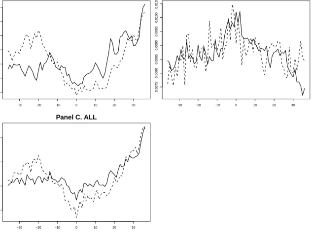
Figure 3.1. plots VOLτ displayed by primary SEOs (depicted in solid lines) and that by secondary SEOs (depicted in dotted lines). In the periods of high SEO volume, Panel A shows that VOLτ is decreasing prior to issuance and attains its minimum at the month of issuance in events of both primary and secondary SEOs. Interestingly, the opposite is observed in the periods of low SEO volume; both primary and secondary SEOs are preceded by increasing VOLτ in Panel B. As a result, Panels A and B conclude that the cross-sectional average of issuance probabilities could be negatively related to the pre-issue
1Independent issuance decisions can be consistent with SEO waves, in that firm’s decision is determined by firm-specific factors as well as market-wide common factors. By decomposing a firm-specific profitability shock into a systematic shock and an idiosyncratic shock, for instance, Pastor and Veronesi (2005) show that the systematic shock triggered by shocks to market-wide common factors shall lead to IPO waves, or equivalently speaking, a clustering of going public, although each firm makes an issuance decision independently on a basis of individual firm-level profitability.
2Denote high- and low-SEO volume by E[NHIGH
t+1 ]and E[NtLOW+1 ]respectively. Then, E[NtHIGH+1 ]>E[NtLOW+1 ] implies that∑Zi=1pHIGHi,t+1 >∑
Z
i=1pLOWi,t+1, wherepiHIGH,t+1 andpLOWi,t+1represents the issuance probabilities in high-and low-SEO volume periods respectively. The assumption of constantZtshall be relaxed in chapter 4.
−30 −20 −10 0 10 20 30 0.0070 0.0075 0.0080 0.0085 0.0090 0.0095 0.0100 Panel A. HIGH V OL −30 −20 −10 0 10 20 30 0.0075 0.0080 0.0085 0.0090 0.0095 0.0100 0.0105 Panel B. LOW −30 −20 −10 0 10 20 30 0.0075 0.0080 0.0085 0.0090 Panel C. ALL
FIGURE 3.1.: Event-time EW Averages of Market Volatility
Panel A reports VOLτ over the 73-month period centered on issue month in high-SEO volume periods. Those in low- and all-SEO volume periods are reported in Panels B and C respectively. VOLτ displayed by primary and secondary SEOs are depicted in solid and dotted lines respectively.
change in market volatility–that is to say, an issuance probability is high when pre-issue market volatility has decreased, but is low when pre-issue market volatility has increased.
In addition, Figure 3.1. shows that the pre-issue dynamics of VOLτ would differ by offering types. An informal eye-ball test of Panel C that is a reproduction of the volatility finding of Carlson et al. (2010), for instance, reveals that secondary SEOs are on average preceded by a greater change in VOLτ relative to primary SEOs. For testing formally if the pre-issue dynamics of VOLτ differs by offering types, I focus on a linear trend in a
time-series of VOLτ, denoted byγ, over the 24-month period prior to issuance. According to Eckbo et al. (2007), the average number of years between the IPO offer date and the SEO as the first post-IPO security offering is 2.31 years. Although no theory predicts an appropriate length of the time interval for this test, I choose the 24-month period by interpreting Eckbo et al. (2007) as evidence that it takes 2.31 years on average for firms to time an equity offering in accordance with changes in market volatility.
In order to test for the null that the linear trend is zero, I perform the Wald-type test of Vogelsang (1998) based on a model
yτ =µ+γ τ+uτ,
whereyτ =VOLτ, uτ =αuτ−1+d(L)eτ, d(L) =∑∞i=0diLi, and eτ ∼i.i.d.(0,σe2). In the presence of general forms of serial correlation, Vogelsang (1998) proposes the Wald-type statistics of t−PS1T andt−PS2T, and claims that t−PS1T has more power butt−PST2 is more robust to a fractionally integrated process. I employ both t−PS1T and t−PS2T to construct a 90% confidence interval forγ throughout the paper.3
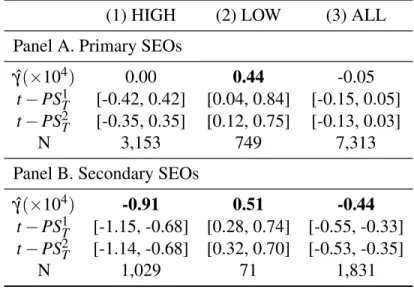
Table 3.1. demonstrates that the pre-issue dynamics of VOLτ statistically differs by the type of shared offered to the public. For instance, columns (1) and (2) of Panel A show that ˆγ in primary SEOs is significant at a 10% level in low-SEO volume periods alone. In secondary SEOs, however, the corresponding columns of Panel B find that ˆγ is significantly negative in the periods of high issuance probability as well as significantly positive in the periods of low issuance probability at a 10% level. Column (3) makes a similar conclusion that, on average, a pre-issue change in VOLτis significantly negative in events of secondary
3Vogelsang (1998) uses 90% confidence intervals for testing a deterministic linear trend. Several finance papers performing the Vogelsang test follow this convention of adopting 90% confidence intervals [See, e.g., Campbell et al. (2001), Xu and Malkiel (2003), Bekaert et al. (2009)].
TABLE 3.1.: Vogelsang Tests
This table performs the Vogelsang tests forH0:γ =0 by runningyτ =µ+γ τ+uτ, where
yτ =VOLτ over 24 months before issuance, uτ =αuτ−1+d(L)eτ,d(L) =∑∞i=0diLi, and
eτ ∼i.i.d.(0,σe2). I use botht−PS1T and t−PS2T to construct 90% confidence intervals for γ, where t−PSiT is defined as T−1(Rβ∗)0
h
R(X0X)−1R0
i−1
(Rβ∗)/ sz2exp(bJTi(m)) fori=1 and 2. Parameters for computingJTi(m)are available on Table II(i) of Vogelsang (1998).
(1) HIGH (2) LOW (3) ALL
Panel A. Primary SEOs ˆ
γ(×104) 0.00 0.44 -0.05
t−PS1T [-0.42, 0.42] [0.04, 0.84] [-0.15, 0.05]
t−PS2T [-0.35, 0.35] [0.12, 0.75] [-0.13, 0.03]
N 3,153 749 7,313
Panel B. Secondary SEOs ˆ
γ(×104) -0.91 0.51 -0.44
t−PS1T [-1.15, -0.68] [0.28, 0.74] [-0.55, -0.33]
t−PS2T [-1.14, -0.68] [0.32, 0.70] [-0.53, -0.35]
N 1,029 71 1,831
SEOs but not of primary SEOs. Overall, Table 3.1. concludes that the volatility timing, or equivalently speaking, a relation between an issuance probability and a pre-issue change in market volatility would be prevalent when making a secondary SEO rather than making a primary SEO. I shall further examine it in chapter 4.
Equally importantly, column (3) of Table 3.1. seems to refute the volatility-timing puzzle of Carlson et al. (2010) who graphically illustrate that on average an event-time EW average of market volatility or VOLτ is decreasing prior to issuance in events of primary SEOs.4 In their paper, the authors improve an original real option-based model of primary
4As noted earlier in this paper, Carlson et al. (2010) also find that market volatility has increased after issuance. While Table 3.1. refers to the first half, chapter 4 shall examine the last half of the volatility finding of Carlson et al. (2010) in terms of the Granger-causality of equity issuance for predicting future market volatility.
SEOs in Carlson et al. (2006) by augmenting commitment-to-invest, and predict that the risk of primary SEO-conducting firms shall be increasing prior to issuance, in that growth options generate riskier cash flows than existing assets-in-place up to the moment when the options are exercised by means of primary SEOs. As an empirical exercise, Carlson et al. (2010) estimate time-varying betas of the conditional capital asset pricing model (CAPM) by running short-window regressions, as originally implemented in Lewellen and Nagel (2006), and find that, on average, the beta is increasing prior to issuance, which is consistent with the model prediction. As recognized by the authors, however, the decreasing market volatility dynamics displayed by primary SEO-conducting firms apparently contradicts the SEO risk dynamics implied by real options theory.
In column (3) of Table 3.1., I find that ˆγ for primary SEOs is insignificantly different from zero at a 10% level. As long as an issuer attempts to time a primary offering with respect to decreasing market volatility over 24 months prior to issuance, as presumed in this paper, this insignificant ˆγ suggests that the claimed volatility-timing puzzle by Carlson et al. (2010) could be statistically suspicious to some degree. Along with it, chapter 4 shall provide additional evidence showing that the issuance decision of a primary SEO is not related to the dynamics of market volatility around events. Therefore, I conclude that the volatility dynamics prior to the primary SEO events is not statistically significant enough to be recognized as the puzzling evidence from the perspective of primary SEO-conducting firm’s risk dynamics implied by real options theory.
CHAPTER IV VOLATILITY TIMING
Chapter 3 gives one an interesting finding that, if it is present, the volatility timing would be more prevalent in selling secondary shares via SEOs. In this chapter, I rigorously examine whether or not an issuance probability is related to the pre- and post-issue dynamics of market volatility, along with other determinants that are presumably related to the motivation behind public equity issuance. In section 4.1, I describe a general test procedure for timing market-wide components in equity issuance. Section 4.2 examines if SEO volume is stationary, which is a critical assumption underlying the test procedures. Later, I construct several empirical proxies reflecting the motivation behind equity issuance in section 4.3. Finally, section 4.4 provides empirical results concerning the volatility timing.
4.1. Test Specification
I follow Pastor and Veronesi (2005) and assume that an issuance decision is made on a basis of the changes in explanatory variables rather than the levels of those, or equivalently speaking, an issuer makes an offering in accordance with recent changes in market conditions rather than cumulative market conditions.1 Thus, I propose the following predictive model
pi,t+1=αi+β
0
i∆ftM, (Equation 4.1.)
1Pastor and Veronesi (2005) provide the theoretical argument on the endogeneity of IPO timing, and predict that a going-public decision shall be related to recent improvements in market conditions since the option to wait becomes less valuable to delay an IPO as market conditions improves. The authors find an empirical support that, for instance, a collective action of going public is critically related to recent market returns, but is unrelated to the level of the aggregate M/B ratio.
where pi,t+1 represents a probability that firm i issues public equity in time t+1, ∆ represents the first difference, and ftM represents a k×1 vector of market-wide factors that are discussed by the previous literature as potential economic determinants affecting
pi,t+1.
It would be ideal to directly measure the unobservable firm-level issuance probability
pi,t+1for each firmiin a set of all potentialZtissuers and then regresspi,t+1on explanatory variables. Although it is appealing, the empirical implementation this way is challenging since the unobservable pi,t+1 is hard to measure correctly. In their logit regressions, for instance, DeAngelo et al. (2010) use the dependent variable that equals one if a firm conducts a SEO in a given year and zero otherwise, and treat it as a proxy for pi,t+1. It should be noted that their logit regressions are possibly subject to a sample selection bias that is induced by incidental truncation–that is to say, their SEO sample does not represent all potentialZtissuers considering SEOs, but instead include only observed firms that have been conducted SEOs for a given sample period.
I use aggregate SEO volume or Nt to avoid this empirical challenge relating to the hardship of measuring pi,t+1 correctly. Given thatNt is persistent but stationary, as shall be shown later, I assume that Nt follows the autoregressive (AR) model of order l, and thus write thatNt−µ =φ1(Nt−1−µ) +· · ·+φl(Nt−l−µ) +ηt, where µ =E[Nt] andηt is a white noise. Invoking a property of the Bernoulli distribution, then, one can write the following regression specification
Nt+1=A0+β0(Zt∆ftM) + l
∑
k=1φkNt−k+1+ηt, (Equation 4.2.)
where A0≡∑Zi=t1αi+µ∑lk=1φk. See Appendix for details. Importantly, Equation 4.2. states that a relationship of SEO volume with the changes in market-wide determinants,
multiplied byZt, effectively reflects a cross-sectional average of firm-specificβi0 or a firm-specific relationship between pi,t+1and∆ftM in Equation 4.1..
Previous studies point out the complex interaction and feedback among variables in Equation 4.2., so that running a single equation without accounting for such complex relations would result in inefficient estimates. For instance, Baker and Wurgler (2000) find that current aggregate issuance activity is negatively related to a future market return. Pastor and Veronesi (2005) find that current IPO volume is positively related to a lagged market return, but is negatively related to lagged market volatility and a future market return. As a result, these complex lead-lag relations shall be investigated in the analysis of simultaneous-equations models instead of running the single regression.
For the efficiency gain, I use a following vector autoregressive (VAR) model
yt =c+Φ1yt−1+Φ2yt−2+. . .+Φpyt−p+εt, (Equation 4.3.)
where yt = (nt,∆fˆtM)0, nt is defined as ln(Nt∗), Nt∗ = max{Nt,0.5}, ∆fˆtM is defined as Zt∆ftM, and εt ∼ i.i.d.(0,Ω). Throughout the paper, the lag length of p shall be selected using Schwart-Bayesian (BIC) information criterion. There are a few remarks on implementing Equation 4.3.. First, I treatA0in Equation 4.2. as a constantcin Equation 4.3. for simplicity. Unreported results show that the main findings of this paper remain unchanged when c is specified as seasoned dummy variables alternatively. Instead of a raw series of Nt, I use nt for suppressing excessive fluctuations of SEO volume which could cause a so-called regression phenomenon. The same treatment is found in Dahlquist and de Jong (2008) applying the log transformation to monthly IPO volume. Finally, Zt is computed as the number of CRSP-listed firms used in computing a CRSP VW market index. Following Lowry (2003), I use the actual number of public firms as estimates of
1972 by assuming that the actual number of public firms grows at the rate of 0.045% per month.
4.2. Stationary Test
For implementing the VAR model specified in Equation 4.3., I first construct two time-series of quarterly SEO volume using 7,313 primary SEOs, denoted by{NP,t}144t=1, and 1,831 secondary SEOs, denoted byNS,t 144
t=1, both of which have been conducted from the period 1Q 1970 – 4Q 2005.
The construction of SEO volume series at a quarterly frequency is conventional [see, e.g., Lowry (2003) and Pastor and Veronesi (2005)]. I follow this convention, in that a monthly time-series of secondary SEO volume contains too many zeros; secondary SEOs have not been made for a total of 45 months over the sample period. The frequent presence of such months with no offerings shall cause a problem with using a simple VAR model because a desirable asymptotic property is hardly achievable in a finite sample. One remedy would be obtained by explicitly specifying a stochastic process of monthly SEO volume via, for instance, a Poisson process [see, e.g., Dahlquist and de Jong (2008)]. In the context of a system of equations, however, this approach brings forth a significant burden of computation, which is simply beyond the scope of this paper.
Since the main assumption underlying Equation 4.2. is the stationarity of a SEO volume series, I check whether a time-series of{Nt}is stationary or nonstationary. For this task, one might simply perform the augmented Dickey-Fuller (ADF) test forH0:{Nt} ∼
I(1).2 However, the sample autocorrelation function of{Nt}verifies that the SEO volume is highly persistent, and thus this persistency could make the use of the ADF test problematic
2In her study of IPO volume fluctuations, Lowry (2003) performs the augmented Dickey-Fuller test and concludes that persistent IPO volume is nonstationary.
since the ADF test is known to have very low power against theI(0) alternatives that are close to being I(1). Accounting for the persistence and achieving the maximum power against the local-to-unit alternative, I instead perform the so-called DF-GLS test proposed by Elliot, Rothenberg, and Stock (1996). Formally speaking, I testH0:π=0 by running a regression that ∆Ntd=πNt−d 1+ k
∑
j=1 πj∆Nt−d j+et, whereNtd =Nt−ψˆ0Dt, ˆψ =argminψ∑(Ntα¯ −ψ 0 Dt)2, and ¯α =1+c¯/144. By settingDt equal to one and ¯cequal to minus seven, I intend to test the null thatNt∼I(1)without drift against the alternative thatNt∼I(0)with nonzero mean since no obvious linear trends are observed in both series of{NP,t}144t=1 andNS,t 144t=1. Following Ng and Perron (2001) for size improvement, furthermore, I selectkask∗=argmink≤kmaxMAIC(k), where MAIC is the modified Akaike information criterion.
Table 4.1. performs the DF-GLS tests. For both SEO volume series, H0 :π =0 is rejected at a 5% level. Thus, it concludes that SEO volume is persistent but stationary, which is consistent with the previous findings of Viswanathan and Wei (2008) and Dahlquist and de Jong (2008).3 As a result, this stationarity of quarterly SEO volume justifies the transition to Equation 4.2.. In an empirical analysis followed on, I shall employ
nP,t andnS,t, wherenP,t andnS,t are defined as ln(NP∗,t)and ln(NS∗,t)respectively. Table 4.1. verifies that the DF-GLS tests for the stationarity of{nt}also reject the null of unit root at a 5% level in both primary and secondary SEOs.
3Viswanathan and Wei (2008) make the same conclusion that the DF-GLS test rejects the null of a unit root in monthly SEO volume. They also reject the null of a unit root in monthly IPO volume at a 5% level. Dahlquist and de Jong (2008) find that a unit root hypothesis of monthly IPO volume is rejected under the ADF test and a stationarity hypothesis of monthly IPO volume is not rejected under the KPSS test.
TABLE 4.1.: DF-GLS Tests
This table performs the DF-GLS test by running∆ydt =πydt−1+∑kj=1πj∆ydt−j+et,where
y ={Nt,nt}, Nt is the number of SEOs in quarter t over the period from 1Q 1970 to 4Q 2005, nt =ln(Nt∗), Nt∗ =max{Nt,0.5}, ytd =yt−ψˆ, ˆψ =argminψ∑(yαt¯ −ψ)2, and
¯
α =1−7/144. For implementing the tests, kis selected as k∗=argmink≤kmaxMAIC(k), where MAIC is the modified Akaike information criterion of Ng and Perron (2001). The t-statistics for testingH0:π=0 are reported in parentheses. The critical values are -2.58 at 1%, -1.95 at 5%, and -1.61 at 10%. Nt nt Offering Type k πˆ R2 k πˆ R2 Primary SEOs 10 -0.29 0.32 12 -0.33 0.37 (-3.00) (-3.34) Secondary SEOs 1 -0.15 0.13 8 -0.15 0.26 (-2.93) (-2.31) 4.3. Empirical Proxies
As a variable of main interest, market volatility or VOLt is computed as the quarterly variance of CRSP daily VW market index returns in quarter t. Along with VOL, I include several proxies for capital demands, information asymmetry, liquidity, and investor sentiment in a vector of market-wide component ftM, none of which is mutually exclusive in explaining SEO decisions.
First, it is well known that primary SEOs are preceded by price run-up. Among others, for instance, Choe et al. (1993) find that more offerings are made in expansionary phases of the business cycle at which market returns tend to increase. Given this well-documented price run-up, I compute the market return, denoted by RETt, by compounding CRSP daily VW market index returns over quarter t, and include it in the vector yt. Pastor and Veronesi (2005) explain why primary IPO waves are preceded by increasing market returns, in that greater capital demands, induced by decreasing expected market
risk premium, lead to more primary offerings. Thus, the capital demand story predicts that RET shall be positively related to the issuance probability of a primary offering. At the same time, however, it should be noted that RET can be influenced by investor sentiment. This implies that the relation of an issuance probability with pre-issue market returns has dual interpretations; SEOs are motivated for the price run-up that reflects either increasing capital demands or increasing investor sentiment.
In semi-strong form efficient, Myers and Majluf (1984) and Lucas and McDonald (1990) hypothesize that information asymmetry induces the adverse-selection costs of issuing equity and, as a result, predict that more firms will conduct equity offerings when information asymmetry is low. Follow-on studies provide empirical support for it. With the notion of time-varying adverse-selection costs, for instance, Korajczyk et al. (1991) find that firms prefer to issue equity just after credible information has released via earnings announcements. According to Bayless and Chaplinsky (1996), the negative announcement effect is lower in magnitude in high SEO volume periods than in low SEO volume periods, which is suggestive of a negative relationship between an issuance probability and market-wide information asymmetry. Although these studies exclusively focuses on primary offerings, the theory of information asymmetry can be equally applied to secondary offerings, in that stakeholders liquidating their positions via secondary SEOs may prefer to sell their own shares when the market is most informed about the fundamental value of their firms.
I consider the dispersion of abnormal returns around public firms’ earnings announcements made in quarter t as a proxy for market-wide information asymmetry prevailing in the corresponding quarter. In practice, I compute the variance of CARi,t for all firms with earnings announcements in quartert, where CARi,t is a three-day cumulative return around each announcement, or equivalently speaking,∑1d=−1(ri,d−rM,d). Assuming
that the magnitude of CARi,t reflects the degree of information asymmetry, Lowry (2003) claims that the dispersion of CARi,t should be positively related to the degree of market-wide information asymmetry.4Unlike Lowry (2003) using the dispersion of CARi,twithout modifications, I extract their innovations by running the AR model of order two on a time-series of Var[CARi,t]over the period 3Q 1971 – 4Q 2005, and then computing the estimated residuals from the AR(2) fit. This is because a time-series of Var[CARi,t]is persistently increasing over time, and its first two sample partial autocorrelation coefficients are non-zero while the rest are insignificantly different from non-zero. Throughout the paper, I take the estimated residual in quarter t as a proxy for market-wide information asymmetry in quartert, denoted by INFOt.
Among others, Amihud and Mendelson (1986) and Pastor and Stambaugh (2003) argue that the expected return is an increasing function of illiquidity, or equivalently speaking, security price is negatively related to illiquidity. This suggests the possibility that an issuer maximizing the wealth of stakeholders in events of equity issuance may have an incentive to conduct an offering when market-wide illiquidity is low so as to minimize trading costs. As a result, it is predicted that an issuance probability shall be positively related to liquidity, so long as the concern about low trading costs is material. Like the SEOs motivated by information asymmetry, one sees that the SEO activity motivated by liquidity is consistent with the notion of market efficiency.
4As a second proxy for information asymmetry, she computes the dispersion of analysts’ annual earnings forecasts for all public firms in the IBES database. Table 3 of Lowry (2003), however, shows that this proxy has a positive coefficient which is insignificant at a 5% level. For this reason, she takes the dispersion of CARi,t as the sole proxy for information asymmetry throughout her paper. In unreported results, I
have the same observation in the VAR analysis; the dispersion of analysts’ annual earnings forecasts has a insignificantly positive coefficient in the VAR models on primary and secondary SEO volume. Since the proxy for information asymmetry should be negatively related to the issuance probability via a channel of adverse-selection costs of issuing equity, this paper also does not consider the dispersion of analysts’ annual earnings forecasts as a proxy for information asymmetry.
For market-wide trading costs, I rely on a price-impact proxy of Amihud (2002) as a measure of market-wide liquidity in quartert, denoted by LQDt.5 Following Watanabe and Watanabe (2007), LQDt is constructed in three steps. First, PRIMj,t is defined as (1/Dj,t)∑Dd=j,t1|rj,d,t|/νj,d,t, whererj,d,t andνj,d,t are the return and dollar volume of stock
j on day d in quarter t and Dj,t is the number of daily observations in quarter t, and is computed for stock j only if (a) it is ordinary common equity exchanged in NYSE and AMEX, (b) Dj,t is greater than 44, and (c) the beginning-of-the quarter price is between $5 and $1,000. Next, the aggregate price impact, APRIMt is computed each quartert as (1/Kt)∑Kj=t1PRIMj,t, where Kt is the number of stocks included in quartert. At the last step, LQDt is computed as the negative estimated residual from the modified AR(2) model of APRIMt that is specified in Watanabe and Watanabe (2007).
Finally, the behavioral literature argues that public equity offering can be motivated by investor sentiment, as asserted by the notion of windows-of-opportunity. With the presence of temporary mispricing due to a limit on arbitrage, the managerial opportunistic behavior suggests that a higher level of market-wide mispricing would lead to more offerings aiming to exploit abnormal profits that are arising during the periods of windows-of-opportunity.
In this paper, a composite index of sentiment, denoted by SENTt, is used to measure market-wide investor sentiment, which is originally proposed in Baker and Wurgler (2006, 2007). By construction, SENTtis the first principal component of six empirical proxies that are known to represent the degree of market-wide mispricing, such as the closed-end fund discount (CEFD), NYSE share turnover (TURN), the number (NIPO) and average first-day returns (RIPO) on IPOs, the equity share in new issues (S), and the dividend premium (PDND).
I first construct the quarterly series of these empirical variables, all of which are available at a monthly frequency in Jeffrey Wurgler’s Website.6 Quarterly CEFDs and PDNDs are computed as monthly CEFDs and PDNDs recorded in March, June, September, and December. TURN in quartertis computed as the average of monthly TURNs in quarter
t. NIPO in quarter t is computed as the sum of monthly NIPOs in quarter t. RIPO in quartert is computed as the weighted average of monthly RIPOs in quartert, where each monthly RIPO is weighted by a corresponding monthly NIPO. Finally, S in quarter t is computed as a ratio of the sum of monthly SEs in quarter t to the sum of monthly SEs plus SDs in quartert, where SE and SD represent aggregate equity and debt respectively. Then, I follow the same procedures of Baker and Wurgler (2006, 2007) and compute the first principal component of the correlation matrix of six quarterly proxies. As a result, a composite sentiment index in quartertis formulated as
SENTt = −0.40CEFDt+0.46TURNt+0.39NIPOt+0.31RIPOt−1 −0.19St−1−0.59PDNDt−1.
Figure 4.1. shows the quarterly time-series of the variables constructed above. Panel A plots a time-series of primary SEO volume (depicted in a solid line) and that of secondary SEO volume (depicted in a dotted line), showing that both volume series have been fluctuated over time and tend to move together; a correlation between primary SEO volume and secondary SEO volume is 0.56. Interestingly, secondary SEOs have been conducted frequently prior to the stock market crash of 1987 and started increasing again since year 2000 that approximately corresponds to the end of the dot-com era. In years surrounding the stock market crash of 1987, market uncertainty was high in Panel B, market
performance was bad in Panel C, market opinions on fundamentals were severely diverged in Panel D, and market liquidity was dried up in Panel E, all of which are consistent with the findings of previous studies on the stock market crash. As a final remark, the quarterly sentiment index in Panel E is qualitatively as same as the annual index of Baker and Wurgler (2006) and the monthly index of Baker and Wurgler (2007) over the period 1970 – 2005.
In implementing Equation 4.3., I normalize all variables ofyt except fornt for having zero mean and one standard deviation, making them in comparable units. Panel A of Table 4.2. reports contemporaneous correlations among five normalized variables of ∆fˆ– ∆[VOL, RET,d ∆INFO,[ ∆LQD, and[ ∆SENT–along with the p-values from the Pearson\ moment tests. There are several notes. First, a positive relation between ∆[VOL and ∆INFO–greater market uncertainty corresponds to greater information asymmetry–would[ be consistent with Chen and Zhao (2009), in that market volatility is driven by unexpected shocks to future cash flows and information asymmetry–the difference between an insider’s view on and a market’s view on a firm’s fundamental value–is a main source of the cash flow shocks.7 Next, ∆LQD is negatively related to[ ∆VOL, which is conformable to the[ bid-ask determination theory; if market volatility falls, the market-wide illiquidity also falls because decreasing uncertainty regarding fundamentals reduces the expected costs of market making. No relation between∆[VOL and∆SENT would support Pastor and Veronesi\ (2005) viewing that a channel between market volatility and market-wide mispricing is unclear. A positive relation between ∆LQD and[ RET is anticipated by Amihud andd Mendelson (1986), in that the expected risk premium is a positive, concave function of illiquidity. ∆SENT is positively related to\ RET, which is not surprising as asserted by thed
7An early study by Campbell (1991) argues that market volatility is mainly driven by discount rate news rather than cash flow news. Chen and Zhao (2006) point out that an omitted-variable bias in a predictive regression for the expected market risk premium would cause a problem with measuring the discount rate news. As a result, they claim that Campbell (1991) treating the cash flow news as the residual could make an incorrect conclusion on the relative importance of discount rate news versus cash flow news.
1970 1975 1980 1985 1990 1995 2000 2005 0 20 60 100 140
Panel A. SEO volume
1970 1975 1980 1985 1990 1995 2000 2005 0e+00 4e−04 8e−04 Panel B. Volatility 1970 1975 1980 1985 1990 1995 2000 2005 −0.2 −0.1 0.0 0.1 0.2 Panel C. Return 1970 1975 1980 1985 1990 1995 2000 2005 −0.005 0.000 0.005 0.010
Panel D. Information asymmetry
1970 1975 1980 1985 1990 1995 2000 2005 −0.02 0.00 0.01 0.02 Panel E. Liquidity 1970 1975 1980 1985 1990 1995 2000 2005 −2 0 2 4 Panel F. Sentiment
FIGURE 4.1.: SEO Volume and Other Empirical Proxies over 1Q 1970 – 4Q 2005 Panel A depicts quarterly primary SEO volume in a solid line and quarterly secondary SEO volume in a dotted line. Panel B reports quarterly market volatility or VOLt. Panel C reports quarterly market returns or RETt. Panel D depicts a measure of quarterly information asymmetry or INFOt. Panel E shows a measure of quarterly liquidity or LQDt. Finally, Panel F shows a measure of quarterly investor sentiment or SENTt.
TABLE 4.2.: Correlations and Variance Inflation Factors (VIFs)
Panel A reports the contemporaneous correlations among∆[VOLt,RETdt,∆INFO[t,∆[LQDt, and ∆SENT\t. The p-values from the Pearson moment tests are reported in parentheses. Panel B reports the VIFs in the case that nt is regressing against ∆[VOLt−1, RETdt−1, ∆INFO[t−1,∆[LQDt−1, and∆SENT\t−1.
∆[VOLt RETdt ∆INFO[t ∆LQD[t ∆SENT\t Panel A. Correlations ∆[VOLt -0.43(0.00) 0.27(0.00) -0.57(0.00) 0.01 (0.92) d RETt 0.15(0.08) 0.42(0.00) 0.17(0.05) ∆INFO[t 0.02 (0.83) -0.19(0.03) ∆[LQDt -0.17(0.04)
Panel B. Variance Inflation Factors
VIF 1.91 1.64 1.29 1.75 1.19
behavioral literature. Finally, a negative relation of∆LQD with[ ∆SENT is understandable,\ in that high liquidity implies low trading costs for implementing the arbitrage strategy of exploiting temporary mispricing and subsequently leads to low investor sentiment [see, e.g., Shleifer and Vishny (1997)]. Overall, I find that the correlations among the variables in Panel A of Table 4.2. are broadly consistent with the findings of previous studies, and thus conclude that the variables successfully capture certain dimensions of market conditions reflecting information asymmetry, liquidity, and investor sentiment.
The strong correlations documented in Panel A of Table 4.2. would indicate that a problem arising from multicollinearity among variables adversely affects statistical inferences on estimated coefficients when the variables are used together as a vector of
yt in the VAR model specified in Equation 4.3.–as their correlations becomes stronger, it becomes more difficult to determine which variables actually influence n. Although it is not irrefutable to test whether the multicollinearity is really causing a problem in explaining
n, I compute the variance inflation factors (VIFs) as diagnostic statistics for detecting the multicollinearity problem in Panel B of Table 4.2..8 When regressingnt against the vector ∆fˆt−1, Panel B shows that ∆[VOL has the greatest VIF of 1.91 and implies that, if the multicollinearity causes a problem, the coefficient on ∆VOL is most likely to have an[ incorrectly underestimated t-statistic.
More importantly, as argued by Greene (2007), the multicollinearity becomes in principle problematic when one has a prior belief that bad data is employed in a good model, where the good model is secured by theory. Among others, a risk-return relation postulated in the asset pricing literature provides one with a good model implying thatRETd is a function of∆[VOL or vice versa. Exactly speaking, the risk-return relation states that the expected market risk premium is functional of conditional market volatility. Theex post
market return has its functional form of the unobservable expected market risk premium. At the same time, a change inex postmarket volatility is also related to the unobservable conditional market volatility. Consequently, the ex ante risk-return relation argues that
d
RET shall be related to ∆[VOL, in that both RET and∆VOL are empirical proxies for the unobservable expected market risk premium.
This predicted relationship between RET andd ∆[VOL, implied by the ex ante risk-return relationship, suggests that the standard error of the estimated coefficient on ∆[VOL shall be adversely affected by its functional relation withRET whenever both variables ared used together in a regression of equity issuance. Regardless of any statistical symptoms indicating how severely the multicollinearity affects the t-statistics of the estimated coefficients on RET andd ∆[VOL, thus, one would like to avoid the case where RET andd
8The VIF for variableb
krepresents an additional increase in the variance ofbkthat can be attributable to
the correlation ofXkwith other explanatory variables,X−k. The use of the VIFs cannot be refutable since no
theoretical argument is available to judge the threshold value that the VIF is high enough to adversely affect the variance of estimates.
∆[VOL are employed together in a single regression, so long as she believes that the asset pricing model of risk-return is gooda priori[see, e.g., Pastor and Veronesi (2005)].
4.4. Empirical Results
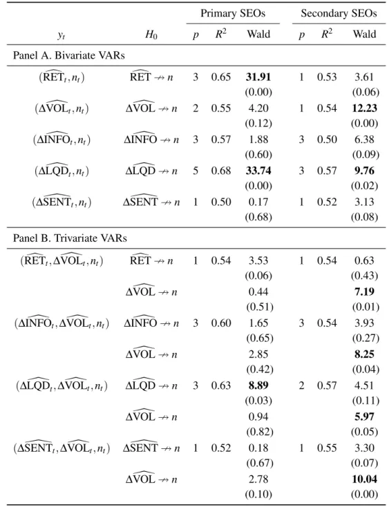
Table 4.3. reports the Granger-causality tests implied by the VAR(p) model fits of bivariate yt in Panel A and those of trivariate yt in Panel B. For instance, H0:RETd 9n states the null hypothesis thatRET does not Granger-caused n. The Wald statistics, corrected for heteroskedasticity, are reported along with the corresponding p-values in parentheses. According to the first two rows of Panel A,RET is useful to predict the issuance probabilityd of a primary offering, while∆VOL is useful to predict that of a secondary offering. In the[ remaining rows,∆INFO and[ ∆\SENT have no predictability for both nPandnS, but∆LQD[ Granger-causes both nP and nS. Without considering an omitted-variable bias, Panel A concludes that timing a SEO significantly differs on the dimensions of RET andd ∆[VOL– that is to say, an issuer shall time market returns when conducting a primary offering, while she shall time changes in market volatility when conducting a secondary offering.
The same conclusion is made on the different timing with respect toRET andd ∆[VOL in Panel B where the predictability is investigated in the trivariate VAR models and thus the omitted-variable bias would be less problematic relative to Panel A. One sees that∆[VOL is useful to predict the issuance probability of a secondary SEO in all four cases whereRET,d ∆INFO,[ ∆[LQD, and∆SENT are each combined with a pair of\ ∆[VOL andn. In contrast, ∆VOL is not useful to predict the issuance probability of a primary SEO in any four cases.[ Overall, Table 4.3. provides preliminary evidence that the volatility timing, if it is present, would be prevalent when conducting a secondary SEO.
Before moving to a multivariate VAR analysis, I compute orthogonalized impulse response functions (IRFs) implied by the bivariate VAR fits in Panel A of Table 4.3., and
TABLE 4.3.: Granger-causality Tests
This table performs the Granger-causality tests implied by the VAR(p) model that yt =
c+Φ1yt−1+. . .+Φpyt−p+εt, whereyt = (nt,∆fˆtM)
0
,∆fˆtM is defined asZt∆ftM, andεt∼
i.i.d.(0,Ω). For instance, H0:RETd 9n states the null thatRET does not Granger-caused
n. BIC information criterion is used for selecting p. The Wald statistics, corrected for heteroskedasticity, are reported along with the corresponding p-values in parentheses.
Primary SEOs Secondary SEOs
yt H0 p R2 Wald p R2 Wald
Panel A. Bivariate VARs
(RETdt,nt) RETd 9n 3 0.65 31.91 1 0.53 3.61 (0.00) (0.06) (∆[VOLt,nt) ∆[VOL9n 2 0.55 4.20 1 0.54 12.23 (0.12) (0.00) (∆INFO[t,nt) ∆INFO[ 9n 3 0.57 1.88 3 0.50 6.38 (0.60) (0.09) (∆LQD[t,nt) ∆LQD[9n 5 0.68 33.74 3 0.57 9.76 (0.00) (0.02) (∆SENT\t,nt) ∆SENT\9n 1 0.50 0.17 1 0.52 3.13 (0.68) (0.08)
Panel B. Trivariate VARs
(RETdt,∆VOL[t,nt) RETd 9n 1 0.54 3.53 1 0.54 0.63
(0.06) (0.43)
∆VOL[9n 0.44 7.19
(0.51) (0.01)
(∆INFO[t,∆VOL[t,nt) ∆INFO[ 9n 3 0.60 1.65 3 0.54 3.93
(0.65) (0.27) ∆[VOL9n 2.85 8.25 (0.42) (0.04) (∆LQD[t,∆VOL[t,nt) ∆LQD[9n 3 0.63 8.89 2 0.57 4.51 (0.03) (0.11) ∆VOL[9n 0.94 5.97 (0.82) (0.05)
(∆SENT\t,∆VOL[t,nt) ∆SENT\9n 1 0.52 0.18 1 0.55 3.30
(0.67) (0.07)
∆VOL[9n 2.78 10.04
examine how the causal impact of an innovation to explanatory variablex, denoted byηx, affects a future issuance probability. For this task, the recursive causal ordering is restricted thatx→n; in words,xaffectsn, butndoes not affectx.
Figure 4.2. reports orthogonalized IRFs ofnwith respect to orthogonalized shocks to d
RET, ∆[VOL, ∆INFO,[ ∆LQD, and[ ∆\SENT respectively. The IRFs of primary SEOs are depicted in solid lines and those of secondary SEOs are depicted in dotted lines. There are two things worth mentioning. First, the IRFs are consistent with the theoretical arguments on how each variable shall be related to an issuance probability. In response to the structural shock to RET, for instance, Panel A plots thatd n jumps immediately and then gradually decreases to zero thereafter. This positive effect is anticipated by the positive effect of price run-up on an issuance probability. The effects ofη∆INFO,η∆LQD, andη∆SENT in Panels C, D, and E are all consistent with the theoretical predictions on their roles in describing an issuance activity; an issuance probability will increase if information asymmetry falls or liquidity increases or investor sentiment increases.
Next, Panel B graphically illustrates that the shock to∆[VOL negatively influences an issuance probability. Interestingly, the effect of volatility shocks on an issuance probability is stronger in secondary SEOs than in primary SEOs; the change innS due to the market volatility shocks is almost twice in magnitude as big as that ofnP. In contrast, the remaining panels show that the structural shocks to other determinants affect almost equally the issuance probabilities of both types of offerings. Thus, Panel B of Figure 4.2. strengthens the findings of Table 4.3., concluding that market volatility shocks are more influential in making a secondary SEO rather than a primary SEO.
Table 4.4. performs the multivariate VAR models and reports the equations for nt. The t-statistics, given in parentheses, are corrected for heteroskedasticity. In column (1) where yt is defined as a vector of RETt,d ∆[VOLt, ∆INFOt,[ ∆LQD[t, ∆SENTt, and\
0 2 4 6 8 10 12
−0.05
0.05
0.15
0.25
Panel A. Innovation: ηRET
0 2 4 6 8 10 12
−0.25
−0.15
−0.05
Panel B. Innovation: ηVOL
0 2 4 6 8 10 12
−0.06
−0.02
0.02
Panel C. Innovation: ηINFO
0 2 4 6 8 10 12 0.00 0.10 0.20 Panel D. Innovation: ηLQD 0 2 4 6 8 10 12 −0.05 0.00 0.05 0.10
Panel E. Innovation: ηSENT
FIGURE 4.2.: Orthogonalized Impulse Response Functions (IRFs)
This figure plots orthogonalized IRFs from the bivariate VAR(p) model fits specified in Panel A of Table 4.3.. The initial ordering condition states that x→ n, where x ∈ n
d
RET,∆[VOL,∆INFO[,∆[LQD,∆SENT\ o
. Panel A plots ∂nt+h/∂ ηRET, where ηRET is an orthogonal shock toRETdt. Panel B plots∂nt+h/∂ ηVOL, whereηVOLis an orthogonal shock to∆[VOLt. Panel C plots∂nt+h/∂ ηINFO, whereηINFO is an orthogonal shock to ∆INFO[t. Panel D plots∂nt+h/∂ ηLQD, whereηLQDis an orthogonal shock to∆[LQDt. Finally, Panel E plots ∂nt+h/∂ ηSENT, where ηSENT is an orthogonal shock to ∆\SENTt. The IRFs are depicted in solid and dotted lines for primary and secondary SEOs respectively.
nS,t, the proxy for investor sentiment has a significantly negative coefficient at a 10% level, meaning that lagged investor sentiment is negatively related to the current issuance probability of a secondary SEO. This apparently counter-intuitive behavior regarding investor sentiment would be consistent with no post-issue abnormal performance of secondary SEO-conducting firms in Panel B of Table 2.1., in that an issuer seems to time a secondary offering when investor sentiment is decreasing and, as a result, secondary shares are sold at prices that are getting close to their fundamental values. As shall be shown in columns (3) and (4), this negative coefficient on ∆SENT\t−1 remains significant in the various equations for nS,t. To my best knowledge, no theory is available to predict this inverse relation between investor sentiment and the issuance probability of a secondary SEO.
Next, column (1) shows that the estimated coefficient on ∆[VOLt−1 is negative but insignificant at a 10% level. If column (1) would be free from the multicollinearity problem, one could conclude that secondary SEOs are rarely motivated by pre-issue dynamics of market volatility. As discussed above, however, the multicollinearity among explanatory variables could cause a statistical problem in column (1) whereRETdt−1and∆[VOLt−1are used together, and thus the t-statistic of the estimated coefficient on ∆[VOLt−1 would be underestimated, although the estimated coefficient is unbiasedly negative. I shall cope with the potential multicollinearity problem in remaining columns.
Concerning that the multicollinearity could matter to some extent in column (1), I first rely on an underfitting approach by dropping eitherRET ord ∆[VOL in a regression equation fornin the VAR setting. Although it is the most common remedy for the multicollinearity problem, however, the underfitting causes the omitted-variable bias unless a discarded variable is not related to retained variables or has no explanatory power for a dependent
TABLE 4.4.: Vector Autoregressive (VAR) Analysis
This table reports various equations fornt in the VAR(p) fits for nP,t and nS,t, where nP,t
andnS,t are defined as the logarithm of primary and secondary SEO volume respectively. In columns, PrinCompt is defined as the first principal component of a vector of RETdt, ∆INFO[t, and∆LQD[t. BIC information criterion is used for selecting p. The t-statistics, reported in parentheses, are corrected for heteroskedasticity.
(1)nS,t (2)nS,t (3)nS,t (4)nS,t (5)nP,t (6)nP,t (7)nP,t (8)nP,t Intercept 0.61 0.57 0.62 0.58 1.19 0.79 1.19 1.15 (3.58) (3.41) (3.70) (3.71) (4.69) (2.59) (4.82) (4.64) d RETt−1 0.06 0.08 0.11 0.10 (0.99) (1.36) (2.32) (2.18) ∆VOL[t−1 -0.05 -0.14 -0.11 0.04 -0.03 -0.03 (-0.62) (-2.04) (-1.79) (0.55) (-0.47) (-0.54) ∆INFO[t−1 -0.08 -0.01 -0.09 -0.10 -0.03 -0.09 (-1.58) (-0.19) (-2.03) (-2.14) (-0.66) (-2.19) ∆LQD[t−1 0.08 0.10 0.10 0.07 0.12 0.05 (1.19) (1.08) (1.84) (1.76) (1.92) (1.49) ∆SENT\t−1 -0.10 -0.09 -0.10 -0.09 -0.03 0.02 -0.03 0.00 (-1.79) (-1.56) (-1.85) (-1.75) (-0.81) (0.56) (-0.81) (0.00) PrinCompt−1 -0.07 -0.07 (-1.34) (-1.60) nt−1 0.71 0.65 0.71 0.73 0.68 0.54 0.68 0.70 (10.02) (6.16) (10.24) (11.85) (10.30) (6.60) (10.59) (10.74) ∆VOL[t−2 -0.13 -0.02 (-1.77) (-0.44) ∆INFO[t−2 0.11 0.02 (1.40) (0.44) ∆LQD[t−2 -0.01 0.03 (-0.14) (0.44) ∆SENT\t−2 -0.04 0.03 (-0.71) (0.58) nt−2 0.07 0.25 (0.71) (2.34) R2 0.54 0.55 0.54 0.56 0.57 0.58 0.57 0.54
variable.9 Note that the underfitting does not induce the omitted-variable bias, so long as the risk-return relation is truea prioriand a correct model of equity issuance consists of the expected market risk premium. Put differently, the omitted-variable bias matters to some extent in the underfitting analysis only when one believes that the correct model of equity issuance consists of bothRET andd ∆[VOL, or equivalently speaking,RET andd ∆[VOL have distinct roles in explaining the motivation behind SEOs.
I drop RET in column (2) butd ∆[VOL in column (3). Column (3) shows that the estimated coefficient on RETdt−1 is insignificantly different from zero at a 10% level, meaning that price run-up has no effect on the issuance probability of a secondary SEO. Recalling that the market-wide capital demands are proxied byRET, no explanatory powerd ofRET in column (3) is understandable by the fact that secondary offerings do not intendd to raise external capitals for initiating new projects. Without taking into account the volatility timing, column (3) finds that a secondary SEO-issuing firm seems to emphasize decreasing information asymmetry, increasing liquidity, and decreasing investor sentiment– the estimated coefficients on∆INFO[t−1, ∆[LQDt−1, and∆SENT\t−1are all significant at a 10% level.
The insignificant coefficient onRETdt−1is interesting in a statistical sense. When the correct model requires both RET andd ∆[VOL, one would be concerned about the omitted variable bias in column (3). Given a trade-off between the precision of estimation and the omitted-variable bias, it is known that the estimated coefficient onRETdt−1is more precise than that in column (1) on a basis of the mean-squared error (MSE) criterion [see, e.g., Greene (2007)]. Although it would be biased, therefore, the insignificant coefficient on
d
RETt−1in column (3) concludes that the correct model explaining a secondary SEO does
9Suppose that a model is correctly specified in a regression thaty=X
1β1+X2β2. Greene (2007) shows that runningyonX1without includingX2results in E[b1] =β1+P12β2,whereP12= (X
0 1X1)−1X
0
1X2. Thus, it is easy to see thatb1is unbiased ifX
0