CAHIER DE RECHERCHE <0915E WORKING PAPER <0915E Département de science économique Department of Economics Faculté des sciences sociales Faculty of Social Sciences
Université d’Ottawa University of Ottawa
When being out of school can be bad for the school:
a case for conditional cash transfers
*Fernanda Estevan
†December 2009
*
I thank Jean-Marie Baland, Jean Hindriks, Eric Verhoogen, David de la Croix, Vincent Vandenberghe, François Maniquet, Susana Peralta, Philippe Van Parijs, Marie-Louise Leroux, Alfonso Valdesogo, Carmen Camacho, Amrita Dhillon, and Olivier Bos for very useful comments at different stages of this research. This paper has been presented at the Doctoral Workshop and Workshop in Welfare Economics at Universite catholique de Louvain, EDP Jamboree in Paris School of Economics, BREAD/CEPR/University of Verona Summer School in Development Economics, Third Annual Conference on Development and Institutions at CEDI Brunel University, and University of Ottawa and has greatly benefited from their participants’ suggestions. I started this research while visiting CERGE-EI, Prague, under a Marie-Curie Host Fellowships for Early Stage Training (EST) in Public Policy, Market Organization and Transition Economies. Financial support from this fellowship is fully acknowledged. All remaining errors are mine.
†
Department of Economics, University of Ottawa, 55 Laurier E., Ottawa, Ontario, Canada, K1N 6N5; Email: [email protected].
Abstract
We develop a theoretical model to analyze how the lack of full enrollment affects the quality of public education chosen by majority voting. In our model, the households choose whether to enrol their child at school or not. Poor households do not send their children to school because there is an opportunity cost related to education. We show that if preferences for public education quality are decreasing in income, an ends against the middle equilibrium may arise with low levels of expenditures. In this setting, the introduction of a conditional cash transfer program may increase the educational budget chosen by majority voting. Indeed, by raising school enrollment, it increases the political support for educational expenditures.
Key words: education, school enrollment, conditional cash transfers, political economy.
JEL Classification: H42, I28, O12.
Résumé
Dans cet article, nous développons un modèle théorique pour analyser comment un taux de participation scolaire faible peut affecter la qualité de l’éducation choisie par vote majoritaire. Dans ce modèle, les ménages décident d’inscrire ou non leurs enfants à l’école. Les ménages pauvres n’envoient pas leurs enfants à l’école à cause du coût d’opportunité lié à l’éducation. Si les préférences pour la qualité de l’éducation publique sont décroissantes dans le revenu, l’équilibre est déterminé par une coalition entre les ménages pauvres et riches et le niveau de dépenses est faible. Dans ce contexte, l’introduction d’un programme de transferts conditionnels peut augmenter le budget de l’éducation choisi par vote majoritaire. En augmentant la participation scolaire, ce programme renforce le support politique pour les dépenses en éducation publique.
Mots clés: éducation, taux de participation scolaire, transferts conditionnels, économie
politique.
1
Introduction
There is a broad agreement on the need to provide universal primary education worldwide, as enshrined in the Millennium Development Goals.1 The main reason put forward is that education is a fundamental component of human capital devel-opment. Moreover, there is an additional argument for why full enrollment should be pursued that has been much disregarded in the literature. It is related to the detrimental impact that the lack of full enrollment may have on the political support for educational expenditures.
Low enrollment is an important issue, even if clear progress has been made in this domain in the past years. Between 1999 and 2005, 24 million children were given access to primary education. Nonetheless, there were still 72 million children out-of-school in 2005, mainly in developing countries (UNESCO, 2008).2
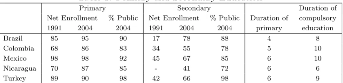
Several educational policies have contributed to increase school enrollment. The basic education system has been expanded in some countries. Legal provisions for compulsory education have been established and tuition fees have been abolished (UNESCO, 2008). While these measures are certainly important, they do not ensure that all children will be at school. Indeed, even countries with free-of-charge schools and compulsory education have been confronted with the lack of full enrollment. Table 1 presents primary and secondary education figures for for selected countries.
Table 1: Primary and Secondary Education
Primary Secondary Duration of Net Enrollment % Public Net Enrollment % Public Duration of compulsory 1991 2004 2004 1991 2004 2004 primary education Brazil 85 95 90 17 78 88 4 8 Colombia 68 86 83 34 55 78 5 10 Mexico 98 98 92 45 67 85 6 10 Nicaragua 70 87 85 - 41 72 6 6 Turkey 89 90 98 42 66 98 6 9
Source: UNESCO Institute for Statistics: http://stats.uis.unesco.org/.
There are several possible explanations for the fact that some children do not receive any education even if schools are publicly available. A prominent reason is that education encompasses a variety of direct and indirect costs. One example is the opportunity cost of education related to foregone child labor earnings.3
The recognition of such costs has given rise to a number of policies designed to stimulate the households’ demand for education. During the 1990s, several
coun-1
http://www.un.org/millenniumgoals/. 2
In 2005, total primary school enrollment was 688 million worldwide (UNESCO, 2008). 3
There is an extensive literature on child labor. Ranjan (1999) and Baland and Robinson (2000) constitute examples of papers highlighting the trade-off between education and child labor.
tries have implemented programs aimed at providing families with incentives to put their children through school, such as conditional cash transfers (CCT). Un-der these programs, low-income households receive a cash transfer if their children attend school. Apart from alleviating poverty in the short term, these programs are intended to have long-lasting benefits by raising the children’s human capital. The Brazilian Bolsa Familia and the Mexican Oportunidades constitute examples ofCCT programs, among others.4
At first sight, the fact that some children are excluded from the school system seems to benefit those currently at school. Indeed, the educational expenditures have to be divided among fewer children, resulting in a higher expenditure per student. While this analysis is correct for a fixed educational budget, it can no longer be applied once one considers that the total amount of educational expenditures reflects the households’ preferences for education. If this is the case, the fact that some children are out of school may have a perverse impact on school expenditures, as a consequence of lack of political support for increased funds for education.
The main purpose of this paper is to show how low enrollment may affect the level of educational expenditures chosen by the households in a political economy framework. In this context, we also analyze the effect of the introduction of a con-ditional cash transfer program on the equilibrium level of educational expenditures. In our model, all the households have the same preferences regarding education and private consumption. However, families are heterogeneous with respect to their income. While education increases their utility, there is an opportunity cost associ-ated to schooling. The latter may be relassoci-ated to foregone child labor earnings or to other indirect costs, such as material and transport. This cost leads poor households to drop their children out of school.
The key element in our argument is that once a household is out of school, it has no incentives to support educational expenditures. Indeed, its utility level is not affected by the quality of schools. In our model, we show that when rich households choose high quality of public education, the preferred level of education is chosen by the median voter and is therefore only indirectly affected by the fact that poor children are out of school. However, if rich households prefer low quality of public
4
There is a growing literature on conditional cash transfer programs. Cardoso and Souza (2004) show that Brazil’sBolsa Familiahad a positive impact on school attendance while the effect in terms of reduced child labor is small. The effects on school attendance were consistent with the micro-simulations’ prediction in Bourguignon et al. (2003). Using data from the MexicanOportunidades, Dubois et al. (2003) find a positive effect in school continuation while Gertler (2004) highlights the improvement in child’s health that can be attributed to the program. de Janvry et al. (2006) discuss the role of conditional cash transfers as safety nets. For a more complete review of the literature on conditional cash transfers, see Das et al. (2005).
education, they may form a coalition with poor households out of school. In this ends-against-the-middle equilibrium, the level of educational expenditures chosen is lower than the level preferred by the median voter.
A related approach is taken by Tanaka (2003) in a model where the households have the choice between education and child labor. Restricting the analysis to the case in which preferences for public education are increasing in income, Tanaka (2003) argues that if the medium voter is out of school, educational expenditures are very low and the level of child labor is huge. This result hangs on public school enrollment rates lower than 50%, what does not seem to be the rule even for de-veloping countries (Table 1). Moreover, the assumption that the preferred level of educational expenditures is increasing in income is restrictive if one considers the possibility of household production of education (Epple and Romano, 1996). In par-ticular, the possibility of supplementing public school with private services, such as tutoring leads to a preferred tax level that is decreasing in income.
Finally, we show that by increasing school enrollment,CCT programs may have a positive effect on the quality of public education. This is a consequence of aug-mented political support for educational expenditures caused by the inclusion of poor households in the school system.
The idea that households not benefiting from a publicly provided good may vote for low expenditures has been already explored in models combining public and pri-vate provision. In these models, public and (higher quality) pripri-vate schools coexist, the latter being chosen by rich households. Stiglitz (1974) was the first to investigate theoretically the consequences of public and private provision of education on the households’ preferences.5
Glomm and Ravikumar (1998) present conditions that ensure the existence of a majority voting equilibrium in this setting. It amounts to assuming that the pre-ferred level of educational expenditures is decreasing in income. Epple and Romano (1996) provide a generalization of this result and shows that if the level of educa-tional expenditures is increasing in income, an ends against the middle equilibrium may arise. In this setting, the poor and rich households join forces and vote for low educational expenditures.6 More recently, de la Croix and Doepke (2009) integrate fertility decisions in the analysis and show that the crowding out of public education spending occurs only if the society is dominated by the rich. Indeed, in a democracy where politicians are responsive to low income families, they argue that the presence
5
For a rigorous discussion on the conditions for the existence of a majority voting equilibrium, see Milgrom and Shannon (1994) and Gans and Smart (1996).
6
Epple and Romano (1996) were also interested in understanding the effect of educational vouch-ers. This issue has been further exploited in related models by Hoyt and Lee (1998), Chen and West (2000), and Cohen-Zada and Justman (2003).
of a large private education sector benefits public schools.7
While we share the methodology of Epple and Romano (1996), we focus on a totally different issue. In our model, education is exclusively provided by the state, but there is an opportunity cost related to its consumption. This cost prevents poor households from going to school and therefore explains the existence of an ends against the middle equilibrium.
This paper is organized as follows. Section 2 presents the model. In Section 3, we analyze the voting equilibrium when households choose the level of educational expenditures and the tax rate. In Section 4 we investigate the impact of theCCT program on the quality of public education chosen by majority voting. In Section 5 we simulate our model and in Section 6 we conclude.
2
The model
2.1 Households
We assume that the economy is composed of a continuum of households that are identical with respect to their preferences. These are defined over private consump-tion,c, and education, which is available at qualitye.8 The households’ preferences are represented by the utility functionU assumed to be increasing, strictly quasi-concave, and twice continuously differentiable.9 Each household has one adult and one child. We impose the following additional assumptions:
Assumption 1. Education is a normal good.
Assumption 2. There is a level of public education quality that renders a household indifferent between no school and public school, i.e.,
∀ c, c′ ≥0, with c > c′, ∃e >0 such that U(c′, e) =U(c,0).
Consequently, ∀e′ > e,U(c′, e′) > U(c′, e) since U is increasing in e. As shown
by Epple and Romano (1994) and reproduced in Appendix A, Assumption 1 implies that the marginal utility of private consumption decreases as its amount increases along an indifference curve, i.e.,
7
Fernandez and Rogerson (1995) also highlight a different mechanism in the context of higher education. In their model, individuals vote on a partial educational subsidy that may benefit only the medium and high income population if its level is not high enough to induce low income households enrollment.
8
For simplicity, we consider that expenditures in education always translate into quality. In reality, the relation between these them is less than evident, as pointed out by Hanushek (2005).
9
Subscripts denote partial derivatives, that is,Uxis the partial derivative of the utility function with respect tox.
dUc dc U (.)= ¯U <0. (1)
Assumption 2 ensures the desirability of education in the sense that every household is ready to sacrifice some consumption in order to obtain it, provided that its quality is substantial. While this assumption simplifies our presentation, it is not essential for our results.
Households are heterogeneous with respect to their income y. We suppose that y∈[y, y] and is distributed according to the density functionf(y). The correspond-ing cumulative distribution function is F(y). We normalize the population size to one. Average (and total) income is denoted byya and the median income by ym.
All households’ incomes are taxed at the constant rate t.10 The government uses the tax revenues to finance the public education system. Public education is freely available at quality eto all households.11 However, not all households go to public schools since acquiring education entails an opportunity cost w. The latter may be related to foregone child labor earnings or to other indirect costs related to schooling.12 The budget constraint of a household using public education is:
ci = (1−t)yi−w. (2)
The utility function of a household using public education is: U(ci, e),
whereci is given by (2). His indirect utility function is then given by:
Ve(e, t) =U((1−t)yi−w, e). (3)
If a household is out of school, its budget constraint is:
ci = (1−t)yi, (4)
since it does not have to pay for the opportunity cost of education. The utility function of a household out of school is:
10
At the end of Section 3, we discuss how our results change if we consider instead a lump sum or consumption tax scheme.
11
By considering one homogeneous public education market, we rule out the possibility that the household’s decision to live in a given community may depend on the quality of public education in that locality (Tiebout, 1956). However, taking into account this possibility seems natural and would constitute an interesting extension to this work.
12
Undoubtedly, school attendance can be combined with some amount of child work, as showed by Cardoso and Souza (2004). Therefore,wdoes not represent full child wages, but only the proportion of it that is incompatible with schooling. Note also that we have assumed that child labor is not taxed. This is realistic since children work mainly in the informal sector.
U(ci,0),
whereci is given by (4). Its indirect utility function is:
V0(t) =U((1−t)yi,0), (5)
and is not affected byesince the household does not participate in the educational system.
A householdicompares (3) to (5) in order to take its enrollment decision. Thus, its utility function is given by:
Υ(e, t, b) = max{U((1−t)yi,0), U((1−t)yi−w, e)}. (6)
Using (6), let Φ(¯e, t, w, yi) be the utility differential between joining or not the school system. It is defined by:
Φ(e, t, w, yi)≡U((1−t)yi,0)−U((1−t)yi−w, e). (7)
2.2 Government
The technology available in this economy is such thateunits of private consumption can be transformed into one unit of education of qualitye, i.e. the price of education is normalized to 1. We require that the government’s budget balances, so that:
tya=eθ (8)
whereθis the enrollment rate.
2.3 Equilibrium
Assumption 2 ensures that there is always a level of public education quality that persuades a household to enroll at school. In Lemma 1, we show that poor house-holds require a higher level of public education quality in order to join the educa-tional system than rich ones. This is related to the diminishing marginal utility of consumption and to the fact that poorer households are less willing to pay for the opportunity cost of education.
Lemma 1. There is a level of education quality, denoted˜ei, which renders household
iindifferent between no school and public school. The levele˜i is decreasing in yi.
Proof. The level of public education quality, ˜ei, that renders householdiindifferent
between not going to school and going to public school in the presence of a CCT program is defined by:
Φ(˜ei, t, w, yi)≡0, (9) using (7). When the level of public education is zero, (7) is positive:
Φ(0, t, w, yi) =U((1−t)yi,0)−U((1−t)yi−w,0)>0. Assumption 2 ensures that there is a level ofedenoted e′ such that:
Φ(e′, t, w, yi) =U((1−t)yi,0)−U (1−t)yi−w, e′
<0.
The continuity of Φ(e, t, w, yi) is ensured by the continuity of the utility function. Moreover, Φ(e, t, w, yi) is monotonic:
dΦ
de =−Ue((1−t)yi−w, e)<0,
so that it crosses the horizontal axis only once. Hence there is a ˜ei that satisfies (9). We next show that ˜ei is decreasing inyi. Applying the implicit function theorem to (9), we can write: ∂˜ei ∂yi =− Φy Φe = (1−t) [Uc((1−t)yi,0)−Uc((1−t)yi−w,e˜)] Ue((1−t)yi−w,˜e) <0, due to (1).
The monotonicity of ˜ei on yi implies the following result:
Corollary 1. If a household ichooses not to go to school, neither do all households
with incomeyj < yi. If a householdiprefers public education to no school, so do all
households with income yj > yi.
Proof. For a household i that strictly prefers no school to public school, we know
that Vie < Vi0, where Ve and V0 are given by (3) and (5). Thus ˜ei is higher than
the level provided, otherwise householdiwould go to school. This will also be true for a household j with income yj < yi, since by Lemma 1 it would require an even higher level of public education quality in order to join the public school.
Consider a household ithat strictly prefers public education to no school, that is,Ve
i > Vi0. This implies that the level of public education available, e, is higher
or equal than ˜ei, defined by (9), otherwise the household would be out of school. By Lemma 1, we know that ˜eis decreasing in income. Thus the level required by a householdj with income yj > yi is lower than ˜ei. Consequently, householdj also opts for public education.
Let yl denote the household that is indifferent between joining or not the edu-cational system for a quality of public education equal toe. Using (7), yl is defined by:
Φ(e, t, w, yl)≡0. (10)
Thus, the proportion of households attending the public school is given by:
θ(e, t) = 1−F(yl). (11)
In order to analyze the behavior of the government budget constraint, suppose an increase ine. Undoubtedly, such an increase in quality attracts additional pupils to the school system. However, the raise in quality requires an increase in the tax rate, reducing the disposable income of all households. Consequently, some low income households drop out of the educational system, unwilling to pay for the opportunity cost of education. There is room for a reduction in taxes. Lemma 2 shows that this last effect is of second order and does not offset the initial increase in the tax rate.
Lemma 2. An increase in the quality of public education always require a raise in taxes.
Proof. The total impact of the quality of public education,e, on taxes,t, is obtained
by totally differentiating (8): de −θ−e∂θ ∂e + dt ya−e∂θ ∂t = 0 dt de = θ+e∂θ∂e ya−e∂θ∂t dt de = θ ya 1 +εθ,e 1−εθ,t (12) where εθ,e = ∂θ∂eeθ and εθ,t = ∂θ∂tθt are the elasticities of the enrollment rate with respect to e and t, respectively. Differentiating (11) with respect to e and t, we have: ∂θ ∂e =−f(yl) ∂yl ∂e. (13) ∂θ ∂t =−f(yl) ∂yl ∂t. (14)
Applying the implicit function theorem to (10), we get: ∂yl ∂e =− Φe Φy = Ue((1−t)yl−w, e) (1−t) [Uc((1−t)yl,0)−Uc((1−t)yl−w, e)] <0, (15)
since the denominator is negative due to (1). We now compute the impact of the tax rate. Applying the implicit function theorem to (10), we obtain:
∂yl ∂t =− Φt Φy = yl 1−t >0. (16)
Combining the signs of (13), (14), (15), and (16), we have: dt
de >0. (17)
3
Voting on the quality of public education and on the
tax rate
In this section, we analyze the household’s choice of the quality of public education, e, that corresponds to a tax rate,t. We start by considering that all the individuals vote. At the end of the section, we discuss how the results would change if there was some level of vote abstention.
Throughout we assume that more than half of the households attend a public school implying that the median income voter chooses a positive level of educational expenditures. This assumption is consistent with most educational systems in de-veloping countries that have public enrollment rates greater than 50%.13 If this was not the case, the prediction of our model would be very similar to the one in Tanaka (2003). Indeed, we should expect very low or even zero educational expenditures, since a positive tax rate could not be the result of a voting equilibrium if less than half of the population benefit from it.
Additionally, we assume that at the median income household preferred level of public education quality, the poorest household chooses not to go to school. These assumptions ensure that the two groups of households actually exist (i.e. out of school and public school).
Consider a household currently at a public school. The slope of its indifference curves (in absolute terms) in the (e, t) space denoted byη(e, t) is:
η(e, t) = ∂U ∂e ∂U ∂t = Ue((1−t)yi−w, e) yiUc((1−t)yi−w, e), (18) using (3). 13
As illustrated in Table 1, Colombia and Nicaragua are the only countries that do not fulfill this requirement for secondary education. This is mainly due to the fact that the total secondary enrollment rates in these countries are very low.
The slope η(e, t) is not necessarily monotonic in y, as shown in (18). With the purpose of determining the voting equilibrium, we impose monotonicity conditions on the preferences over the expenditure-tax bundle (e, t) for the households attending public school. We suppose that their preferred level of (e, t) either increases or decreases with income for those households at school. Clearly, two opposite effects influence their preferences. On the one hand, rich households favor a higher quality of public education because education is a normal good. This is the so-calledincome effect. On the other hand, the rich pay a larger fraction of educational expenditures under proportional income taxation. Since any increase in quality requires a raise in taxes, richer households support decreases in the quality of education in order to reduce their tax burden. This corresponds to the substitution effect. If the income effect is larger (resp. smaller) than the substitution effect, the richer the household the larger (resp. smaller) its preferred level of the expenditure-tax bundle. We present the detailed analysis of both effects, based on Kenny (1978), in the Appendix B. We show that which effect dominates depend on the relative magnitudes of the income elasticity of education and the elasticity of substitution between consumption and education. The first case we study corresponds to the preferred bundle of expenditure-tax increasing with income.
Proposition 1. If the preferred bundle of expenditure-tax increases with income for the households at school, the majority voting equilibrium is the median income voter’s preferred tax rate.
Proof. Let (tm, em) be the expenditure-tax bundle preferred by the household with
median income among those belonging to the government budget constraint. It is given by: Ue((1−tm)ym−w, em) ymUc((1−tm)ym−w, em) = θ ya 1 +εθ,e 1−εθ,t ,
where the right-hand side is given by (12). To prove our claim, we show that (tm, em) defeats any bundle with more or less educational expenditures. Consider a bundle (t′, e′) representing a higher level of expenditures than (tm, em). All the households
at school with income lower than the median i.e., with y ∈ [yl, ym], prefer (tm, e) to (t′, e′). This is a consequence of the assumption that the preferred bundle of
expenditure-tax increases with income. Similarly, the households out of school i.e., those withy ∈[y, yl], also prefer (tm, em) to (t′, e′) in order to decrease taxes since
their utility is not affected by the quality of public education. Since these two groups represent half of the electorate, (tm, em) defeats (t′, e′). The same claim can be done
the preferred bundle increases with income, all the households with income higher than the median prefer (tm, em) to (t′′, e′′). Since they are 50% of the voters, (tm, em) beats (t′′, e′′).
If all households were at school, the median income voter preferred bundle would be the voting equilibrium. Indeed, the monotonicity conditions imposed on the preferences ensure single-crossing of the utility function given by (3). The fact that some households decide not to join the educational system does not alter the voting equilibrium under the assumption that the preferred bundle is increasing in income. This happens because the households not going to school and voting for small quality would anyway be the ones preferring the lower expenditure-tax bundle under this assumption. Therefore, the fact that they do not go to school does not affect the voting equilibrium.
We now turn to the case in which the preferred bundle of expenditure-tax de-creases with income for those households attending public school. The median in-come household’s preferred tax rate cannot be the majority voting equilibrium in this setting. All the households with income higher than the median would be in favor of a marginal decrease in the expenditure-tax bundle. Similarly, all the house-holds out of school would support the same marginal decrease since they do not benefit from the educational system. If there is an equilibrium, it will be given by a tax level decided by a coalition grouping the poorer and richer households. In this ends against the middle equilibrium, educational expenditures will be lower than the level chosen by the median voter.
This result is strictly related to the failure of the single-crossing condition of the utility function (6). In this case, the preferred bundle is decreasing in income. Thus, the poor households should be the ones supporting the highest expenditures in education. However, since they are out of school, they support low educational expenditures. Therefore, they join forces with the rich that also prefer low expendi-tures under the assumption that the preferred bundle is decreasing in income. We derive necessary conditions for an interior majority voting equilibrium in Proposition 2.
Proposition 2. If the preferred bundle is decreasing in income and there is a ma-jority voting equilibrium, it corresponds to the bundle in the government budget
constraint most preferred by a household yˆ. Between this pivotal voter, yˆ, and the
household indifferent between no school and public school,yl, there is exactly half of
the population.
Proof. The proof consists of two parts. We first suppose that at points on the
that half of the population is located between them. The second part shows that the existence of households yl and ˆy is essential for all candidate points to be an equilibrium.
Households with income y ∈ [yl,yˆ] strictly prefer to go to public school than to be out of school, according to Corollary 1. If the preferred bundle is decreasing in income, they would prefer a marginal increase in the expenditure-tax bundle to (ˆe,ˆt). If these households constitute the majority of the population, such a marginal increase defeats point (ˆe,ˆt).
Now consider households with incomey >yˆ. If the preferred bundle is decreasing in income, they prefer a marginal decrease in the expenditure-tax bundle to (ˆe,ˆt). Households with incomey < yl would also prefer a decrease in the expenditure-tax bundle since they are out of school. Thus, if they are majority, a marginal decrease in the expenditure-tax bundle defeats bundle (ˆe,ˆt). Hence, given the existence of householdsyl and ˆy at a point on the government budget constraint, there must be exactly half of the population between them for it to be an equilibrium.
The existence of householdylis ensured by the assumption that the lowest income household is out of school at the median income preferred level of expenditure-tax. In addition, if there is a household ˆyit must have an income higher thanyl, otherwise it would not have public school as its preferred choice. The non-existence of household ˆ
y precludes the existence of an equilibrium.14
Therefore, we may expect that those systems in which school enrollment is not widespread and the preferred level of expenditures is decreasing in income, the total educational budget is lower than if all the children were at public schools. Clearly, this does not imply that the amount spent by student is necessarily lower. Indeed, the educational expenditures are divided over a smaller number of pupils when enrollment is not total.
While the conditions stated in Proposition 2 are necessary, they are not sufficient for the existence of a majority voting equilibrium. The main difficulty in establishing a majority voting equilibrium in this setting is related to the absence of single-crossing in (6). To see this, consider the case of a household currently out of school. While he is opposed to a marginal increase in the quality of public education, he may vote for a large increase of it provided that it allows him to enter school. On the contrary, a middle income voter may favor a small increase of the quality but will most probably be against large increases. The candidate point is an equilibrium if the group that favors a large increase is smaller than the one against it. Ultimately, the fact that a given level of education quality satisfying Proposition 2 is an equilibrium
14
depends on the preferences and on the income distribution. In Section 5, we simulate the model in order to determine whether there is an equilibrium choice ofe. In all the exercises we have performed, the candidate point satisfying the necessary conditions appear as a majority voting equilibrium.
We now briefly discuss how our results change if one considers that public educa-tion is financed through other tax schemes. We start by considering the hypothetical case in which the government could impose a lump sum tax on all households. In this case, only the income effect is present. Indeed, the tax paid by each individual is unrelated to its income level. Thus, the preferred level of educational expenditures is monotonically increasing and the result in Proposition 1 always apply under the Assumption that education is a normal good. Another possibility is to consider that the tax is levied on consumption rather than on income. This is especially relevant in the context of developing countries where indirect taxes frequently constitute an important part of the tax revenues. Moreover, this reinforces the fact that all the households help financing the educational system, since one may argue that income taxes are normally not paid by very poor individuals. With commodity taxation, the results would be very similar except that child labor would be also taxed in this case.
In our model, the private sector is ruled out from the analysis. However, we can speculate how the results would change if one allowed for the existence of private schools in this model. While the private sector is generally small in developing countries, this may apply to some countries that have more private schools. As in Epple and Romano (1996) and in other papers mentioned above, the introduction of private schools would reduce the political support for public education expenditures by the rich households. Thus, one should expect a generalization of the ends against the middle result. Indeed, under both monotonicity assumptions, the poor and rich households would form a coalition and vote for low taxes.
Throughout we have assumed that all the individuals in this economy vote. In reality, some households do not vote, even when voting is compulsory. Clearly, if turnout is unrelated to the households’ characteristics, our results are unchanged. However, if the decision to go voting is related to the household’s income or schooling level, our results may change. The literature on developed countries shows a positive relation between income/ education and the probability to go voting. Few empirical studies investigate this issue in the context of developing countries. Fornos et al. (2004) investigate voting turnout in several Latin American countries. Their results suggest that voting turnout is not influenced by socioeconomic variables. In any case, the introduction of voting abstention correlated with income/ education level should be straightforward. Suppose that in an extreme case, all the households
out of school do not go voting. In this case, the majority voting equilibrium would correspond to the preferred level of the median voter among those households voting.
4
The introduction of a conditional cash transfer
In this Section, we analyze the impact of the introduction of aCCT program on the equilibrium level of educational expenditures. We assume that the CCT program grants a cash transfer equal to b if the household attends school. For the sake of interest, we restrict our analysis to the case in which the cash transfer partially compensates its recipients for the opportunity cost of education, i.e.,b < w.
We assume that theCCT program isuniversal, so that all households attending school are eligible to it. In reality, CCT programs are means-tested since there is a maximum income threshold in order to be eligible to it. However, considering
an universal program greatly simplifies the exposition without altering the main
results. In the presence of a CCT program, the budget constraint of a household using public education is:
ci = (1−t)yi−w+b, (19)
and its indirect utility function becomes:
Ve(e, t, b) =U((1−t)yi−w+b, e). (20)
We assume that the CCT program is financed by taxes. The government budget constraint becomes:
tya= (e+b)θ (21)
A householdicompares (5) to (20) in order to take its enrollment decision. Thus, its utility function is given by:
Γ(e, t, b) = max{U((1−t)yi,0), U((1−t)yi−w+b, e)}. (22)
Using (22), let Ψ(e, t, b, w, yi) be the utility differential between joining or not the school system when aCCT program is in place:
Ψ(e, t, b, w, yi)≡U((1−t)yi,0)−U((1−t)yi−w+b, e). (23)
Clearly, a cash transfer that completely compensates for the opportunity cost of education,b=w, induces full enrollment for any positive level of public education. In such a case, Ψ(e, t, b, w, yi)<0. Moreover, the poorer the household, the higher the level of cash transfer needed to persuade him to join the school system. This
is due to the diminishing marginal utility of consumption. Consequently, if the cash transfer only partially compensates the household for the opportunity cost of education, the CCT program may not be able to achieve full enrollment. Indeed, for very poor households, Φ(e, t, b, w, yi) > 0 for every value of b < w. This is particularly true if the level of public education quality, e, is not high enough to induce full enrollment, as we have assumed in Section 3.
We now turn to our main result concerning the effect of a CCT on the total amount of resources devoted to public education.
Proposition 3. If the preferred bundle of expenditure-tax is decreasing in income, an increase in the conditional cash transfer raises the level of public education ex-penditures obtained by majority voting.
Proof. Letyp denote the income level of the household indifferent between no school
and public school in the presence of a CCT program. Using (23) it is defined by
Ψ(e, t, b, w, yp) = 0. Consider the impact of an increase inb onyp. It is given by:
∂yp ∂b =− Ψb Ψy = Uc((1−t)yp−w+b, e) (1−t) [Uc((1−t)yp,0)−Uc((1−t)yp−w+b, e)] <0. (24)
With an increase in the CCT, the voter indifferent between going to school or not moves to the left. Proposition 2 states that between this household and the pivotal household, ˆy, should be located half of the population in order to (ˆe,ˆt) to be an equilibrium. Therefore, if the increase in b displaces yp to the left, the new ˆy (if it exists) also moves to the left, corresponding to a lower income level. Since the preferred level of the expenditure-tax bundle is decreasing in income, its preferred choice corresponds to a higher level of educational expenditures.
Proposition 3 shows that a CCT program may increase the support for large expenditures in public education by allowing low income households to join the educational system. This is true under the assumption that the preferred bundle of expenditure-tax is decreasing in income. The new pivotal voter is located more to the left and therefore it prefers a higher level of public educational expenditures compared to the previous situation. However, even if the tax rate increases, the amount of resources per student will not necessarily be higher. Indeed, part of the budget is used to finance the conditional cash transfer. Moreover, an increased cash transfer benefit attracts new students to the educational system, potentially decreasing the amount of resources per student. In Section 5, we simulate the model for different values of the cash transfer.
5
Simulation
In this Section we simulate the model in order to determine whether we have a global majority voting equilibrium under the assumption that the preferred bundle of expenditure-tax is decreasing in income. As shown in Appendix B, this case corresponds to an elasticity of substitution between education and consumption higher than the income elasticity of education. We first investigate the existence of a point satisfying the necessary conditions stated in Proposition 2. Then, we verify whether this point is a global majority voting equilibrium by comparing it to several other points in the government budget constraint.
In this simulation15, we define our parameters in order to fit as close as possi-ble the Brazilian data. For simplicity, we assume that the income distribution is log-normally distributed, lny ∼ N(µ, σ2). The parameters of the income distribu-tion are calculated in order to provide an annual mean and median income equal to R$20,400 and R$10,800, which correspond to the values obtained in the 2006 Brazilian Household Survey. These amount to µ= 2.38 and σ = 1.27 if income is measured in thousands. This corresponds to a Gini coefficient of 0.534, very simi-lar to the actual Gini coefficient calculated by IBGE equal to 0.528 in 2006.16 We simulate our model using the CES utility function:
U(c, e) = [βeρ+ (1−β)cρ]. (25) As shown in Appendix B, the preferred bundle of expenditure-tax is decreasing in income for a CES utility function whenever ρ > w−b
yi .
17 We calibrate our utility function in order to obtain roughly 85% of students enrolled at school. We arbitrarily fix the opportunity cost of education toR$650.18
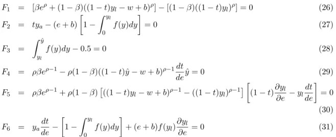
A bundle (e, t) satisfying the necessary conditions given in Proposition 2 is the solution to the following system of non-linear equations:
15
We usedMathematica to perform the simulations presented in this paper. The code is available upon request from the authors. We thank Dennis Epple and Richard E. Romano for providing us with their simulation code that was a great source of inspiration.
16
The Gini coefficient of a lognormal distribution is given by the ratio of standard deviation over the mean. The actual Gini coefficient is calculated by IBGE, Instituto Brasileiro de Geografia e Estatistica, Brazilian Institute of Geography and Statistics, www.ibge.gov.br.
17
In order to verify whether this condition holds, we have to check ifρ > w−b
yl , sinceyl is the
household with the lowest income to enter school. In all the simulations we have performed, this was always the case.
18
Bourguignon et al. (2003) estimate the annual child labor earnings to be around R$960 and
R$1,560. However, they recognize that school attendance can be combined with some amount of child work. Since we take into account only the part of the child labor earnings that is incompatible with schooling, we have chosen a value for the opportunity cost of education that is much lower than the observed child wages.
F1 = [βeρ+ (1−β)((1−t)yl−w+b)ρ]−[(1−β)((1−t)yl)ρ] = 0 (26) F2 = tya−(e+b) 1− Z yl 0 f(y)dy = 0 (27) F3 = Z yˆ yl f(y)dy−0.5 = 0 (28) F4 = ρβeρ−1−ρ(1−β)((1−t)ˆy−w+b)ρ−1 dt deyˆ= 0 (29) F5 = ρβeρ−1+ρ(1−β) ((1−t)yl−w+b)ρ−1−((1−t)yl)ρ−1 (1−t)∂yl ∂e −yl dt de = 0 (30) F6 = yadt de − 1− Z yl 0 f(y)dy + (e+b)f(yl)∂yl ∂e = 0 (31)
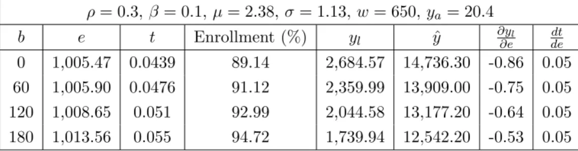
We present some results in Tables 2 and 3 for values ofbranging from 0 to 180. These results confirm the predictions obtained in the theoretical model. The higher the cash transfer, the more low income pupils can join the educational system. The increase in enrollment shifts the pivotal voter to the left of the income distribution. Since the preferred bundle of expenditure-tax is decreasing in income, the poorer the pivotal voter, the higher its preferred tax rate. In our results, this implies an increase in the expenditures per student, meaning that the increase in the tax rate is high enough to compensate for additional students. The key difference between these two cases is the elasticity of substitution between education and consumption equal to 1.66 and 1.43, respectively. A lower elasticity of substitution means that the households consider education and consumption as more complements and therefore the enrollment rate and the preferred level of education are higher.
ρ= 0.4,β = 0.1,µ= 2.38, σ= 1.13, w= 650, ya= 20.4 b e t Enrollment (%) yl yˆ ∂yl ∂e dt de 0 444.40 0.0136 62.62 7,513.79 39,276.40 -10.45 0.04 60 466.56 0.0177 68.65 6,243.89 29,501.80 -8.20 0.04 120 487.37 0.0222 74.58 5,122.09 23,455.30 -6.38 0.05 180 514.90 0.0274 80.53 4,090.98 19,179.10 -4.77 0.05
Table 2: Choice ofefor a given level ofb.
The conditions specified in equations (26) to (31) are necessary but not suffi-cient for an equilibrium. A majority voting equilibrium requires that the candidate point defined by the system of equations receives more than half of the votes when confronted to all the other possible points belonging to the government budget
con-ρ= 0.3,β = 0.1,µ= 2.38, σ= 1.13, w= 650, ya= 20.4
b e t Enrollment (%) yl yˆ ∂y∂el dedt
0 1,005.47 0.0439 89.14 2,684.57 14,736.30 -0.86 0.05 60 1,005.90 0.0476 91.12 2,359.99 13,909.00 -0.75 0.05 120 1,008.65 0.051 92.99 2,044.58 13,177.20 -0.64 0.05 180 1,013.56 0.055 94.72 1,739.94 12,542.20 -0.53 0.05
Table 3: Choice ofefor a given level ofb.
straint. In order to verify this, let (e, t) be the expenditure-tax bundle preferred by the pivotal voter, ˆy and defined by equations (26) to (31). Take (˜e,˜t) to be any alternative expenditure-tax bundle. This point has to belong to the government budget constraint, by satisfying the two equations:
K1 = β˜eρ+ (1−β)((1−t˜)˜yl−w+b)ρ − (1−β)((1−˜t)˜yl)ρ = 0 (32) K2 = ˜tya−(˜e+b) 1− Z y˜l 0 f(y)dy = 0 (33)
Let yk be the individual indifferent between public school at (e, t) and (˜e,˜t). It is defined by: [βeρ+ (1−β)((1−t)yk−w+b)ρ]− βe˜ρ+ (1−β)((1−t˜)yk−w+b)ρ = 0 (34) Suppose first that (e, t) > (˜e,˜t). Since the preferred bundle of expenditure-tax is decreasing in income, we know thatyk>yˆ. All the households with income higher than yk prefer (˜e,˜t) to (e, t). The households with income lower than yk compare public school at (e, t) with no school at (˜e,˜t), since in the latter case they pay lower taxes. Define yj as the household indifferent between being out of school at (˜e,˜t) and public school at (e, t). It is given by:
[βeρ+ (1−β)((1−t)yj−w+b)ρ]−
(1−β)((1−˜t)yj−w+b)ρ
= 0 (35) The political support for (e, t) against (˜e,t˜) come from the households with income between yj and yk. Thus, in order for (e, t) to be a majority voting equilibrium when compared to inferior levels of expenditure-tax, at least half of the population has to have income between yj and yk. Now consider that (e, t) < (˜e,˜t). In this case,yk<yˆ. Householdj is now defined as:
βe˜ρ+ (1−β)((1−t˜)yj −w+b)ρ
−[(1−β)((1−t)yj)ρ] = 0 (36) Now, the voters supporting (e, t) against (˜e,˜t) are those with income higher thanyk or smaller thanyj. Thus, they have to constitute more than half of the voters when (e, t) is compared to all alternatives representing a higher expenditure-tax bundle.
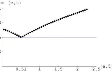
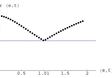
In all the simulations we have done, (e, t) appeared to be a global majority voting equilibrium. It has always been preferred to alternative bundles by a majority of voters in a pairwise comparison. Figures 1 and 2 illustrate the typical results we have obtained. They correspond to the cases presented in Tables 2 and 3 when the cash transfer is equal to 180.
0.51 1 1.5 2 2.5He,t L 0.25 0.5 0.75 1
Vote for He,tL
Figure 1: Voting for (e, t) against (˜e,t˜) whenρ= 0.4 andb= 180.
6
Conclusion
In this paper we assume that the level of public education expenditures is related to the household’s preferences. We show that the fact that some households are out of school may cause a reduction in the quality of public education. If preferences for public education are decreasing in income, poor and rich households may form a coalition and vote for low expenditures. In this setting, the introduction of aCCT program may actually improve the quality of public education. Indeed, by providing the access of low income households to the educational system, theCCT program may influence the voting equilibrium in favor of increased educational expenditures. This mechanism seems to be much ignored in many of the discussions related
0.5 1.01 1.5 2 He,t L 0.25 0.5 0.75 1
Vote for He,tL
Figure 2: Voting for (e, t) against (˜e,t˜) whenρ= 0.3 andb= 180.
to education policy. It is often argued that increasing the quality of education should be a prerequisite for the increase in enrollment. Similarly, much of critics against the conditional cash transfer programs argue that the quality of education is too low to justify sending children to school. This model shows that it may be hard to obtain an increase in the quality of education if the households are not at school. The incentives for policymakers to concentrate resources in education are very low if a large proportion of the population is out of school. Therefore, to start by increasing school enrollment may be a good strategy since it may change the priorities of policymakers and lead to an improvement in the quality of education.
References
Baland, J. M. and Robinson, J. A. (2000). Is child labor inefficient. Journal of Political Economy, 108(4):663–679.
Bourguignon, F., Ferreira, F. H. G., and Leite, P. G. (2003). Conditional cash trans-fers, schooling, and child labor: Micro-simulating brazil’s bolsa escola program. The World Bank Economic Review, 17(2):229–254.
Cardoso, E. and Souza, A. P. (2004). The impact of cash transfers on child labor and school attendance in brazil. Working Paper Vanderbilt University, 04-W07. Chen, Z. and West, E. G. (2000). Selective versus universal vouchers: Modeling
me-dian voter preferences in education. The American Economic Review, 90(5):1520– 1534.
Cohen-Zada, D. and Justman, M. (2003). The political economy of school choice: linking theory and evidence. Journal of Urban Economics, 54(2):277–308.
Das, J., Do, Q.-T., and Ozler, B. (2005). Reassessing conditional cash transfer programs. The World Bank Research Observer, 20(1):57–80.
de Janvry, A., Finan, F., Sadoulet, E., and Vakis, R. (2006). Can conditional cash transfer programs serve as safety nets in keeping children at school and from working when exposed to shocks? Journal of Development Economics, 79(2):349– 373.
de la Croix, D. and Doepke, M. (2009). To segregate or to integrate: education politics and democracy. The Review of Economic Studies, 76(2):597–628.
Dubois, P., de Janvry, A., and Sadoulet, E. (2003). Effects on school enrollment and performance of a conditional transfers program in mexico. Department of Agricultural & Resource Economics, UC Berkeley, Working Paper Series, 981. Epple, D. and Romano, R. E. (1994). Ends against the middle: Determining public
service provision when there are private alternatives. Working paper, University of Florida.
Epple, D. and Romano, R. E. (1996). Ends against the middle: Determining public service provision when there are private alternatives.Journal of Public Economics, 62(3):297–325.
Fernandez, R. and Rogerson, R. (1995). On the political economy of education subsidies. The Review of Economic Studies, 62(2):249–262.
Fornos, C. A., Power, T. J., and Garand, J. C. (2004). Explaining voter turnout in latin america, 1980 to 2000. Comparative Political Studies, 37(8):909–940. Gans, J. S. and Smart, M. (1996). Majority voting with single-crossing preferences.
Journal of Public Economics, 59(2):219–237.
Gertler, P. (2004). Do conditional cash transfers improve child health? evidence from progresa’s control randomized experiment. AEA Papers and Proceedings, 94(2):336–341.
Glomm, G. and Ravikumar, B. (1998). Opting out of publicly provided services: A majority voting result. Social Choice and Welfare, 15(2):187–199.
Hanushek, E. A. (2005). The economics of school quality. German of Economic Review, 6(3):269–286.
Hoyt, W. H. and Lee, K. (1998). Educational vouchers, welfare effects, and voting. Journal of Public Economics, 69(2):211–228.
Kenny, L. W. (1978). The collective allocation of commodities in a democratic society: a generalization. Public choice, 33(2):117–120.
Milgrom, P. and Shannon, C. (1994). Monotone comparative statics. Econometrica, 62(1):157–180.
Ranjan, P. (1999). An economic analysis of child labor.Economics Letters, 64(1):99– 105.
Stiglitz, J. E. (1974). The demand for education in public and private school systems. Journal of Public Economics, 3(4):349–385.
Tanaka, R. (2003). Inequality as a determinant of child labor. Economics Letters, 80(1):93–97.
Tiebout, C. M. (1956). A pure theory of local expenditures. Journal of Political Economy, 64(5):416–424.
UNESCO (2008). Education for all by 2015, will we make it? EFA Global Monitoring Report.
A
Proof of Diminishing Marginal Utility
Proof. This proof follows Epple and Romano (1994). Along an indifference curve,
we know that:
Ucdc+Uede= 0. (37)
The marginal utility of private consumption is given byUc(c, e). Differentiating this expression with respect tocand replacing (37), we obtain:
dUc dc U(.)= ¯U =Ucc−Uc UeUce. (38)
Assume thatpe units of private consumption can be transformed into one unit of consumption. The maximization problem of the household is:
maxU(c, e) s.t. c=y−pe. (39)
At any point (c, e) satisfying U(c, e) =U, the equilibrium condition implies that:
−pUc(y−pe, e) +Ue(y−pe, e) = 0. (40)
Totally differentiating (40) with respect toeand y, we can compute the response of eto a change iny:
de
dy =
pUcc−Uec
Uee−2pUec+p2Ucc. (41)
The denominator is negative due to the assumption of strict quasiconcavity of the utility function. This becomes more explicit once we replace p using (40). The assumption that e is a normal good implies that de
dy >0. Hence, the numerator is negative, or, using (40):
pUcc−Uec = Ue
UcUcc−Uec<0. (42)
Replacing (42) into (38), we obtain: dUc dc U (.)= ¯U = Uc Ue Ue UcUcc−Uec <0, (43)
what yields the result.
B
Elasticity
In this Section, we show that the desired level of public education expenditures increases (resp. decreases) with income whenever the income elasticity of education
is larger (resp. smaller) than the elasticity of substitution between e and c. The proof follows closely Kenny (1978) We then illustrate the results in our case for a CES utility function.
Consider an individual with a utility function U defined over consumption of a numeraire, c, and education of quality e. For simplicity, assume there is no condi-tional cash transfer program, that is, b = 0. Normalizing the price of c to 1 and usingqi to denote the price of epaid by householdi, its budget constraint is:
ci =yi−w−qie.
Since education is publicly provided and financed through proportional taxation, the price paid by each consumer depends on its income. The equilibrium of the government budget constraint in the absence of a conditional cash transfer program implies that:
t=eθ
ya
The cost of the provision of education for a household is:
tyi=eθ
yayi
Therefore the price of education of qualityefor an individual is:
qi= θyi
ya. (44)
Lete(q, y) be the demand function for educational services, where we eliminate the subscripts to simplify the notation. Totally differentiating it with respect toyyields:
de dy = ∂e ∂y + ∂e ∂q dq dy
Multiplying the equation by ye and the last term by qq obtains: de dy y e =ηey+εeq dq dy y q
where ηey = ∂y∂eye is the income elasticity of education and εeq = ∂e∂qqe is the price elasticity of the uncompensated demand for education. The last term in the right-hand side can be calculated using (44):
dq dy y q = θ ya y q = 1 Then,
de dy y
e =ηey+εeq (45)
The assumption that education is a normal good impliesηey >0. Thus,
de dy y e > 0 ⇔ ηey > εeq (46) de dy y e < 0 ⇔ ηey < εeq (47)
Similarly, the above conditions can be expressed in terms of the elasticity of substi-tution. The Slutsky equation of the demand forewith respect to q gives:
∂e ∂q = ∂e ∂q U= ¯U −e∂e ∂y, (48)
or, by multiplying through by qe and the last term by yy to obtain it in elasticity terms:
εeq =ξeq−ηey(1−α) (49)
whereξeq =∂q∂eqe
U= ¯U is the price elasticity of the compensated demand for educa-tion andα= yc is the proportion of income spent on private consumption. In order to computeξeq, consider a price change that is compensated by an income change that leaves the utility level unchanged. We get:
dU =Ucdc+Uede= 0. Since Uc Ue = 1 q, we can write: dc+qde= 0.
Multiplying both sides of this equation by dq1 qceyce yields:
α dc dq q c U= ¯U + (1−α) de dq q e U= ¯U = 0 αξcq + (1−α)ξeq= 0 (50)
By definition, the elasticity of substitution between the numeraire and education, σ, is:
σ= dlog(e/c)
dlog(1/p)|U= ¯U =ξcq−ξeq (51) Combining (50) and (51), we obtain:
ξeq=−ασ (52) Replacing (52) into (49) and then substituting the resulting equation into (45), we obtain: de dy y e =α(ηey−σ) (53) de dy y e > 0 ⇔ ηey > σ (54) de dy y e < 0 ⇔ ηey < σ (55)
B.1 Example: CES Utility Function
Consider the following utility function:
U(ci, e) =βeρ+ (1−β)cρi, (56)
whereci = (1−t)yi−w+b.
The elasticity of substitution,σ, is given by:
σ = 1
1−ρ (57)
The income elasticity of the demand for education is: ηey = yi yi−w+b (58) de dy y e > 0 ⇔ ρ < w−b yi (59) de dy y e < 0 ⇔ ρ > w−b yi (60)