UCD GEARY INSTITUTE
DISCUSSION PAPER SERIES
Generalized Extreme Value Regression
for Binary Rare Events Data: an
Application to Credit Defaults
Raffaella Calabrese
Geary Institute
University College Dublin
Silvia Angela Osmetti
Department of Statistics
University Cattolica del Sacro Cuore, Milan
Geary WP2011/20
September 2011
UCD Geary Institute Discussion Papers often represent preliminary work and are circulated to encourage discussion. Citation of such a paper should account for its provisional character. A revised version may be available directly from the author.
Any opinions expressed here are those of the author(s) and not those of UCD Geary Institute. Research published in this series may include views on policy, but the institute itself takes no institutional policy positions.
Binary Rare Events Data: an Application to
Credit Defaults
Raffaella Calabrese and Silvia Angela Osmetti
Abstract
The most used regression model with binary dependent variable is the logistic re-gression model. When the dependent variable represents a rare event, the logistic regression model shows relevant drawbacks. In order to overcome these drawbacks we propose the Generalized Extreme Value (GEV) regression model. In particular, in a Generalized Linear Model (GLM) with binary dependent variable we suggest the quantile function of the GEV distribution as link function, so our attention is focused on the tail of the response curve for values close to one. The estimation procedure is the maximum likelihood method. This model accommodates skewness and it presents a generalization of GLMs with log-log link function. In credit risk analysis a pivotal topic is the default probability estimation. Since defaults are rare events, we apply the GEV regression to empirical data on Italian Small and Medium Enterprises (SMEs) to model their default probabilities.
1 Introduction
Many of the most significant event in several areas are rare events - in economics and finance, in medicine and epidemiology, in meteorology and natural science and in international relations. In economics and finance, some pivotal applications of the extreme value theory and the rare event methodology are credit risk, Value At
Raffaella Calabrese
University College Dublin, Ucd Casl Belfield Office Park, Dublin 4, e-mail: [email protected]
Silvia Angela Osmetti
University Cattolica del Sacro Cuore, 1, Largo Gemelli, 20123 Milan e-mail: [email protected]
Risk and financial strategy of risk management (Embrechts et al., 1997; Dahan and Mendelson, 2001; Finkenstdt and Holger, 2003; Barro, 2009). In the natural science and in epidemiology the rare events as natural disasters and the epidemics occur infrequently but they are considered of great importance (Frei and Schar, 1998; Roberts, 2000). In international relations, revolutions, massive economic depres-sion and economic shocks are rare events (King and Zeng, 2001). Methodology for modelling occurrence of a rare event is well established. The Poisson distribution is generally used to model the frequency of rare events (see Falk, et al., 2010). In Gen-eralized Linear Models (GLMs) literature the log-linear model is commonly used to model independent Poisson counts (McCullagh and Nelder, 1989).
We consider binary rare events data, i.e. binary dependent variables with a very small number of ones. In GLM literature (see McCullag and Nelder, 1989; Dobson and Barnett, 2008) several models for binary response variable have been proposed by considering different link functions: logit, probit, log-log and complementary log-log models. However, the most used model for binary variables is the logistic regression. The logistic regression shows same important drawbacks in rare events studies: the probability of rare event is underestimated and the logit link is a symmet-ric function, so the response curve approaches zero as the same rate it approaches one. Moreover, commonly used data collection strategies are inefficient for rare event data (King Zeng, 2001). The bias of the maximum likelihood estimators of logistic regression parameters in small sample sizes, that has been well analysed in literature (McCullagh and Nelder, 1989: Mansky and Lerman 1977; Hsieh Mansky and McFadden, 1985), is amplified in the rare event study. Most of these problems are relatively unexplored by literature (King and Zeng, 2001).
The main aim of this paper is to overcome the drawbacks of the logistic regression in rare events studies by proposing a new model for binary dependent data with an asymmetric link function given by the quantile function of the Generalize Extreme Value (GEV) random variable. In the extreme value theory, the GEV distribution is used to model the tail of a distribution (Kotz Nadarajah, 2000; Coles, 2004). Since we focus our attention on the tail of the response curve for the values close to 1, we have chosen the GEV distribution. In GLMs (Agresti, 2002) the log-log and the complementary log-log link functions are used since they are asymmetric functions. In particular, the log-log link function is the quantile function of the Gumbel ran-dom variable. The inverse function of the complementary log-log is one minus the cumulative distribution function of the Gumbel random variable.
The present paper is organized as follows. The next section explains the main draw-backs of the logistic regression model for rare events data. In Section 3 the GEV model for binary rare events data is proposed. The subsection 3.1 presents the Weibull regression model as a particular case of the GEV model. Finally, in Sec-tion 4 we apply our proposal to empirical data to estimate the default probability in credit risk analysis. In particular, the first subsection describes the dataset of Italian Small and Medium Enterprises (SMEs) and the second subsection shows the estima-tion results by applying the GEV model to these data. In the following subsecestima-tion, the predictive accuracies of the logistic regression model and the GEV model are compared for different sample percentages of rare events. Finally, the last section is
devoted to conclusions. In appendix, we report the score functions and the Fisher information matrix of the parameters of the GEV model.
2 The main drawbacks of the logistic regression for rare events
data
LetY1,Y2, ...Yi, ...,Ynbe Bernoulli independent random variables that are equal to
one with probabilityπiand zero with probability(1−πi)fori=1,2, ...,n. A
Gener-alized Linear Model (GLM) considers a monotonic and twice differentiable function
g(·), calledlink function, and a covariate vectorxisuch that g(π) =β0xi.
By applying the inverse function ofg(·), it results that
πi=g−1(β0xi).
In the logistic regression model the probabilityπiis a logistic cumulative
distribu-tion funcdistribu-tion π(xi) = exp(β0xi) 1+exp(β0xi) (1) with β0= [β0,β1, ...,βk] x0= [1,x1, ...,xk].
By applying the inverse function to the equation (1), the logistic link function is the transformation used for the linearity
logit(π(xi)) =ln π(xi) 1−π(xi) =β0xi
The maximum likelihood method is usually used to estimate the parameters vector β.
The logistic regression shows important drawbacks when we study rare events data. Firstly, when the dependent variable represents a rare event, the logistic regression could underestimate the probability of occurrence of the rare event. Secondly, com-monly used data collection strategies are inefficient for rare event data (King and Zeng, 2001). In order to overcome this drawback the choice-based or endogenous stratified sampling (case-control design) is used. The strategy is to select onY by collecting observations for whichY=1 and a random selection of observations for whichY =0. This sampling method is usually supplemented with a prior correction of the bias of MLE estimators. An alternative procedures is the weighting the data to compensate the differences in the sample and population fractions of ones induced by choice-based sampling by the weighted exogenous sampling maximum estima-tor. Manski and Lerman, (1977), McCullagh and Nelder (1989) show a analytical
approximation for the bias in the MLE estimates to account for finite sample. This bias is amplified in application with rare events. Thirdly, the logit link is symmetric about 0.5 logit(π(xi)) =ln π(xi) 1−π(xi) =−logit(π(xi)) =−ln π(xi) 1−π(xi) .
This means that the response curve forπ(xi)approaches zero at the same rate it
approaches one. If the dependent variable represents a rare event, a symmetric link function is not appropriated. Since a counting rare event is usually modelled by a Poisson distribution, which has positive skewness, it is coherent to choose an asym-metric link function in order to obtain a response curve that approaches zero at a different rate it approaches one.
In rare events data values one of the dependent variable are more informative than zero, this follows by the variance matrix
V(βˆ) = " n
∑
i=1 πi(1−πi)x0ixi #−1 .The part of this matrix affected by rare events is the factorπi(1−πi). Most rare
events applications yield small estimates ofP{Yi=1|xi}=πifor all observations.
However, if the logit model has some explanatory power, the estimate ofπiamong
observations for which rare events are observed (i.e. for whichYi=1) will usually
be larger, and closer to 0.5, because probabilities in rare events studies are normally very small, than among observations for whichYi=0. The result is thatπi(1−πi)
will usually be larger for ones than zeros and so the variance will be smaller. In this situation, additional ones will cause the variance to drop more and hence are more informative than additional zeros.
For this reason, in this paper, we focus our attention on the tail of the response curve for the values closed to one.
3 The Generalized Extreme Value (GEV) regression model
Extreme value theory is a robust framework to analyse the tail behaviour of distribu-tions. Extreme value theory has been applied extensively in hydrology, climatology and also in the insurance industry (Embrechts et al., 1997). Embrechts (1999, 2000) considers the potential and limitations of extreme value theory for risk management. Without being exhaustive here, De Haan et al. (1994) and Danielsson and de Vries (1997) study quantile estimation. Bali (2003) uses the GEV distribution to model the empirical distribution of returns. Mc Neil (1999) and Dowd (2002) give an ex-tensive overview of extreme value theory for risk management.Unlike the normal distribution that arises from the use of the central limit theorem on sample average, the extreme value distribution arises from the limit theorem of
Fisher and Tippet (1928) on extreme values or maxima in sample data. The class of GEV distributions is very flexible with the tail shape parameterτcontrolling the shape and size of the tails of the three different families of distributions subsumed under it. The three families of extreme value distributions can be nested into a sin-gle parametric representation, as shown by Jenkinson (1955) and von Mises (1936). This representation is known as the Generalized Extreme Value (GEV) distribution and its cumulative distribution function is given by
FX(x) =exp ( − 1+τ x−µ σ −1τ) −∞<τ<∞, −∞<µ<+∞ σ>0 (2) defined onSX={x: 1+τ(x−µ)/σ >0}. The parameterτ is a shape parameter, whileµandσ(>0)are location and scale parameters respectively.
The Type II (Fr´echet-type distribution) and the Type III (Weibull-type distribution) classes of the extreme value distribution correspond respectively to the caseτ>0 andτ<0, while the Type I class (Gumbel-type distribution) arises in the limit as τ→0. The corresponding distributions of(−X)are also called extreme value distri-butions. We underline that Fr´echet and Weibull distributions are related by a change of sign.
In this paper we propose a generalization of the log-log model by using the quantile function of the GEV distribution as link function. For this reason we call this pro-posal Generalized Extreme Value (GEV) regression model.
For a binary response variable Yi and the vector of explanatory variables xi, let
π(xi) =P{Yi=1|xi}. Since we consider the class of GLMs, we suggest the GEV
cumulative distribution function as the response curve
π(xi) =exp{−[1+τ(β0xi)]−1/τ}. (3)
with
β0= [β0,β1, ...,βk] x0= [1,x1, ...,xk].
Forτ→0 the previous model(3)becomes the response curve of the log-log model and forτ>0 it becomes the Weibull response curve, a particular case of the GEV one.
The link function of the GEV model is given by
[−lnπ(x)]−τ−1 τ
=β0x (4)
that represents a noncanonical link function.
For the interpretation of the parametersβ andτ, we suppose that the value of the j -th regressor (wi-th j=1,2, ..k) is increased by one unit and all the other independent variables remain unchanged. Letx∗the new covariate values, whereasxdenotes the original covariate values. From the equation (4) we deduce that βj=g(π(x∗))− g(π(x))with j=1,2, ..,k. This means that if the parameterβj (with j=1,2, ..k)
the estimate π(x)decreases. Otherwise, if βj is negative, by increasing the j-th
regressor the estimateπ(x)of the GEV model also increases.
Moreover, we analyse the parameter β0: for all fixed values ofτ and for a null independent variable,β0have a positive monotonic relationship with the estimate of
π(x). Finally, we analyse the influence of theτparameter onπ(x). We find that for β0=0 and by considering null values for all the covariates, from the GEV model we
obtain an estimateπ(x)that is about equal toe−1for all the values ofτ. This means thatπ(x)variations depend on the covariate variations and not onτvariations. We propose to estimate the parameters of these models by the maximum likelihood method. LetY= (Y1,Y2, ...,Yn)a simple random sample of sizenfromY, the
log-likelihood function is l(β,τ) = n
∑
i=1 n −yi[1+τ(β0xi)]−1/τ+ (1−yi)ln[1−exp{−[1+τ(β0xi)]−1/τ}] o . (5) Some simulation studies are developed to verify the existence of maximum of the likelihood function, considered as a function of only one parameter for fixed values of the other parameters (likelihood profile function).The score functions, obtained by differentiating the log-likelihood function with respect to the known parametersβ andτ(see Appendix) are give by
∂l(β,τ) ∂ βj =− n
∑
i=1 xi j ln[π(xi)] 1+τ β0xi yi−π(xi) 1−π(xi) j=0,1, ...,k, (6) ∂l(β,τ) ∂ τ = n∑
i=1 1 τ2ln(1+τ β 0x i)− β0xi τ(1+τ β0xi) yi−π(xi) 1−π(xi) ln[π(xi)]. (7)Since the inverse of the link function (3) is a cumulative distribution function only for the values{xi: 1+τxi>0}, in order to identify the maximum likelihood
esti-mates, we apply a constrained optimization with{xi: 1+τ β0xi>0}The asymptotic
standard errors of the maximum likelihood estimators of the parameters in the mod-els are given by the Fisher’s information matrix (see Appendix). Since the Fisher in-formation matrix is not a diagonal matrix (see Appendix), the maximum likelihood estimators of the parametersβ andτ are dependent and they cannot be computed separately.
Since the score functions do not have closed-form, the maximum likelihood esti-mators need to be obtained by numerically maximizing the log-likelihood function using a constrained nonlinear optimization algorithm. The optimization algorithms require the specification of initial values to be used in iterative scheme.
Our suggestion is to use as initial point estimate forτ a value closed to zero. For this value the GEV model becomes the log-log model. Hence, in order to obtain the initial point estimate forβ, we analyse the log-log or Gumbell regression model (see Agresti, 2002) with the response curve
We compute the log-likelihood function of the Gumbel regression l(β) = n
∑
i=1 {yiln[π(xi)] + (1−yi)ln[1−π(xi)]} (9) = n∑
i=1{yiln[exp[−exp(β0xi)]] + (1−yi)ln[1−exp[−exp(β0xi)]]}
=
n
∑
i=1{yi[−exp(β0xi)] + (1−yi)ln[1−exp[−exp(β0xi)]]}.
The score functions are given by
∂l(β) ∂ βj = n
∑
i=1 xi jln[π(xi)] yi−π(xi) 1−π(xi) j=0,1, ...,k. (10)To identify the initial values forβ, we chooseβj∗=0 for j=1, ...,k. By substituting β∗j =0 forj=1, ...,kin equation (9) we obtain
β0∗=ln[−ln(y)].
We use the initial values proposed for the log-log model in order to identify the initial values β∗for the GEV regression model. In particular, we propose to use τ∗'0,β∗j =0 for j=1, ...,kandβ0∗=ln[−ln(y)].
Afterwards, by substituting the initial values for the parameterβ in the equation (6) for j=0 we obtain the estimate ofτ for the first step of the iterative procedure. By using such estimate ofτin the equation (6), we obtain the estimates ofβjwith
j=0,1, ...,kfor the first step in the GEV regression.
3.1 Weibull regression for binary data
A particular case of the GEV cumulative distribution function (2) forτ>0 is the Weibull cumulative distribution function
F(x) =exp ( − −x−µ σ k) x>µ −∞<µ<+∞ σ>0 k>0, (11)
whereµandσ(>0)are, respectively, a location and a scale parameters andkis a shape parameter.
By considering the Weibull cumulative distribution function (11) in the GLM for binary dependent variable, the response curve of the Weibull regression model is
wherek>0. The response curve of the Weibull regression model (12) is a partic-ular case of the GEV response curve (3) forτ>0. On the one hand, the Weibull response curve is an asymmetric function, analogously to the response curve (8) of the Gumbel regression model. On the other hand, unlike the Gumbel response curve (8), theπ(xi)in the Weibull model(12)approaches 1 sharply and approaches
0 slowly. In particular, the behaviour of Weibull response curve depends onk: if
kincreasesπ(xi)approaches sharper both 0 and 1. If the value of the j-th
regres-sor (with j=1,2, ..k) is increased and all the other independent variables remain unchanged, the Weibull response curve (12) decreases whenβj>0 and increases
whenβj<0. The link function of the Weibull regression model
ln 1 π(xi)
1/k
=β0xi. (13)
is a noncanonical link function.
We compute the log-likelihood function of the Weibull regression
l(β,k) = n
∑
i=1 {yiln[π(xi)] + (1−yi)ln[1−π(xi)]} (14) = n∑
i=1 {−yi(β0xi)k+ (1−yi)ln[1−exp(−(β0xi))k]}.The score functions are given by
∂l(β,k) ∂ βj =−k n
∑
i=1 xi j ln[π(xi)] β0xi yi−π(xi) 1−π(xi) j=0,1, ...,k, (15) ∂l(β,k,y) ∂k =−k n∑
i=1 ln[π(xi)]ln[β0xi] yi−π(xi) 1−π(xi) . (16)In order to apply an iterative algorithm, we need to identify the initial valuesβ∗and
k∗for the parameters. Our suggestion is to usek∗=1,βj∗=0 forj=1, ...,kand
β0∗=ln 1−n y . (17)
We obtain the initial value (17) by substitutingβ∗j =0 for j=1, ...,kandk∗=1 in (15) for j=0. We highlight that the Weibull regression with k=1 is a log-linear model whose response curve is the cumulative distribution function of an exponential random variable (McCullagh and Nelder, 1989).
4 An Application to Credit Default
Credit risk forecasting is one of the leading topics in modern finance, as the bank regulation has made increasing use of external and internal credit ratings (Basel Committee on Banking Supervision, 2005). Statistical credit scoring models try to predict the probability that a loan applicant or existing borrower will default over a given time-horizon, usually of one year. According to the Basel Committee on Banking Supervision (2004), banks are required to measure the one year default probability for the calculation of the equity exposure of loans. In this framework, banks adopting the Internal-Rating-Based (IRB) approach are allowed to use their own estimates of PDs. Moreover, Basel II requires these banks to build a rating sys-tems and provides a formula for the calculation of minimum capital requirements where the PD is the main input. For that reason, in many credit risk models such as CreditMetrics (Gupton et al., 1997), CreditRisk+ (Credit Suisse Financial Products, 1997) or CreditPortfolioView (Wilson, 1998), default probabilities are essential in-put parameters.
Altman (1968) was the first to use a statistical model to predict default probabil-ities of firms, calculating his well known Z-Score using a standard discriminant model. Almost a decade later Altman et al. (1977) modified the Z-Score by extend-ing the data-set to larger-sized and distressed firms. Besides this basic method, more accurate ones such as logistic regression, neural networks, smoothing nonparamet-ric methods and expert systems have been developed and are now widely used for practical and theoretical purposes in the field of credit risk measurement (Hand and Henley 1997a, b).
SMEs play a very important role in the economic system of many countries and particularly in Italy (about 90% of Italian firms are SMEs (Vozzella, Gabbi 2010). Furthermore, a large part of the literature (Altman, Sabato 2006; Ansell and al. 2009; Ciampi, Gordini 2008; Vozzella, Gabbi 2010) has focused on the special character of small business lending and the importance of relationships banking for solving information asymmetries. The informative asymmetries puzzle affects particulary SMEs for their difficulty to estimate and make known their fair value. Therefore, the lending to SMEs is riskier than to large corporates (Altman, Sabato 2006; Dietsch, Petey 2004; Saurina, Trucharte 2004). As a consequence, Basel II (BCBS, 2004) establishes that banks should develop credit risk models specifically addressed to SMEs. Only a few studies consider SMEs (Andreeva et al., 2011; Alt-man and Sabato, 2007; AltAlt-man et al. 2010; Hu and Ansell, 2007) since the gathering of SMEs data is quite difficult. Discriminant analysis and logistic regression have been the most widely used methods for constructing scoring systems for SMEs (e.g. Hand and Henley, 1997a, b; Hand and Niall, 2000).
In this paper we propose the GEV regression model in order to overcome the draw-backs of the logistic regression for rare events. Since defaults in credit risk analysis are rare events, we apply the GEV model to empirical data on Italian SMEs to model the default probability. Compliant to Basel II, the default probability is one year forecasted. Therefore, letYtbe a binary r.v. such that
Yt=
1,if a firm is default at timet; 0,otherwise.
and let xt−1 be the covariate vector at time t−1. In this application we aim at
estimating the conditional probability of default
π(xt−1) =P(Yt=1|xt−1)
by applying and comparing the GEV and the logistic regression models.
4.1 The data set
Data used in our analysis comes from AIDA-Bureau van Dijk, a large Italian fi-nancial and balance sheets information provider. We consider defaulted and non defaulted SMEs over the years 2005−2009. In particular, since the default proba-bility is one year forecasted, the covariates concern the period of time 2004−2008. The database contains accounting data of around 210,000 Italian firms with total as-set below 10 millions euro (Vozzella and Gabbi, 2010). From the sample we exclude the firms without the necessary information on the covariates.
Often default definitions for credit risk models concern single loan defaults of a company versus a bank, as also emerges from the Basel II instructions. This is the case for banks building models based on their portfolio data, that is relying on sin-gle loans data which are reserved (e.g., Altman and Sabato (2005) develop a logit model for Italian SMEs based on the portfolio of a large Italian bank). However, traditional structural models (i.e. Merton, 1974) refer to a firm-based definition of default: a firm defaults when the value of the assets is lower than the value of the liabilities, that is when equity is negative. In this work default is intended as the end of the firms activity, i.e. the status, where the firm needs to liquidate its assets for the benefit of its creditors. In practice, we consider a default occurred when a specific firm enters a bankruptcy procedure as defined by the Italian law. The reason for this choice lies in the data availability.
In according with Altman and Sabato (2006) on this dataset we apply a choice-based or endogenous stratified sampling. In this sampling scheme data are stratified by the values of the response variable. We draw randomly the observations within each stratum defined by the two categories of the dependent variable (1=default, 0=non-default) and we consider all the defaulted firms. Then, we select a random sample of non-defaulted firms over the same year of defaults in order to obtain a percentage of defaults in our sample as close as possible to the default percentage (5 %) for Italian SMEs (Cerved Group, 2011). In order to analyze the properties of our model for different probabilities of the rare eventP{Y =1}, we consider also a default percentage of 1%.
By applying the choice-based sampling, the observations are dependent. Since the sample sizes of this application are high, according to the superpopulation theory
(Prentice, 1986) we can consider all the examined samples as simple random sam-ples.
4.2 The estimation results
We apply the GEV regression model proposed in this work to the AIDA database. This application is interesting since it concerns SMEs, on which the availability of data is very difficult, in the Italian credit market, which could be different from other countries.
In order to model the default event, we choose the independent variables that repre-sent financial and economic characteristics of firms according to the recent literature (Vozzella and Gabbi, 2010; Ciampi and Gordini, 2008; Altman et al., 2006). These covariates cover the most relevant aspects of firm’s operations: leverage, liquidity and profitability.
Firstly, we consider 16 covariates: liquidity ratio, current ratio, leverage, solvency ratio, debt/EBITDA, return on equity, return on investment, turnover per employee, added value per employee, cash flow, banks/turnover, debt/equity ratio, return on solvency, EBITDA/turnover, total personnel costs/added value, cash flow/turnover. Secondly, we examine the multicollinearity and we remove the variables with a Vari-ance Inflation Factor higher than 5 (Greene, 2000, p.257-258). Thirdly, by applying the GEV model 7 variables are significant at the level of 5% for the PD forecast:
• Solvency ratio: the ratio of a company’s income over the firm’s total debt obliga-tions;
• Return on investment: the ratio of the returns of a company’s investments over the costs of the investment:
• Turnover per employee: the ratio of sales divided by the number of employees;
• Added value per employee: the enhancement added to a product or service by a company divided by the number of employees;
• Cash flow: the amount of cash generated and used by a company in a given period;
• Bank loans over turnover: short and long term debts with banks over sales vol-ume net of all discounts and sales taxes;
• Total personnel costs over added value: the ratio of a company’s labour costs divided by the enhancement added to a product or service by a company.
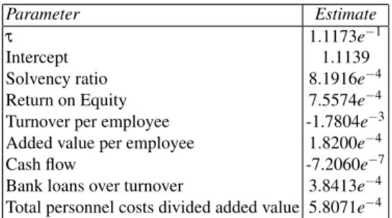
In order to avoid the overfitting, data are randomly divided into two parts: a sample on which the regression models are estimated and a control sample on which we evaluate the predictive accuracy of the models. The Table 1 reports the parameter estimates obtaining by applying the GEV model to the sample of 1485 defaulters and 29700 non-defaulters over the years 2005−2008.
In section 3 we explain the interpretation of the parameters of the GEV model. According to these interpretations we can analyse the influence of each variable in Table 1 on the PD estimate.
Parameter Estimate τ 1.1173e−1
Intercept 1.1139 Solvency ratio 8.1916e−4
Return on Equity 7.5574e−4
Turnover per employee -1.7804e−3
Added value per employee 1.8200e−4
Cash flow -7.2060e−7
Bank loans over turnover 3.8413e−4
Total personnel costs divided added value 5.8071e−4
Table 1 Parameter estimates using the sample of Italian SMEs (1485 defaulters and 29700 non-defaulters) over the years 2005−2008.
At first, Ansell et al. (2009) explain that the solvency ratio should have an inverse relationship with the PD estimate, coherently with our result but in contrast with Ansell et al.’s (2009) result. The return on equity and the added value per employee show the same kind of relationship with the PD, the first result coincides but the second one is in contrast with Ciampi and Gordini (2008). We highlight that our result for the added value per employee coincides with the expectations.
On the contrary, the turnover per employee and the cash flow show a direct rela-tionship with PD, coherently with Altman and Sabato (2006), Ciampi and Gordini (2008). The last two results in Table 1 are in contrast with the expectations: bank loans divided turnover and total personnel costs divided added value show an inverse relationship with the PD estimate. For this reason we analyse the results obtained in literature for these two variables. Ciampi and Gordini (2008) obtain a direct rela-tionship of bank loans divided turnover with the PD estimate. Alternatively, Altman and Sabato (2006) consider the short term debt over equity book value to model the PD and they show that this variable has an inverse relationship with the PD esti-mate, analogously to our result. On the contrary, Fantazzini and Figini (2009) show that the short term debt has a direct influence on PD, coherently with the expecta-tion. Ciampi and Gordini (2008) consider also total personnel costs divided added value in their regression model but their analysis shows a result coherent with the expectations and in contrast with the one showed in Table 1. Fantazzini and Fig-ini (2009) consider also labour costs in their model. In particular, they introduce the personnel expenses over sales in the regression model and this variable shows a direct influence with the PD estimate.
4.3 Forecasting accuracy
We compare the predictive accuracy of the GEV regression model here proposed with the one of logistic regression model. The predictive accuracy of these models is assessed using two performance measures: the Mean Square Error (MSE) and the Mean Absolute Error (MAE), defined as
MSE=1 n n
∑
i=1 (yi−yˆi)2 MAE= 1 n n∑
i=1 |yi−yˆi|. (18)whereyi and ˆyi are the actual and the predicted dependent variable on loani,
re-spectively. Models with lower MSE and MAE forecast the dependent variable more accurately.
The identification of defaulters is a pivotal aim for bank internal models. The rea-son is that it is much more costly to classify a SME as non-defaulter when it is a defaulter that to classify a SME as non-defaulter when it is a defaulter. In particular, when a defaulted firm is classified as non-defaulter by scoring model, banks give it a loan. If the borrower becomes defaulter, the bank may lose the whole or a part of the credit exposure. On the contrary, when a non-defaulter is classified as defaulter, bank loses only interest on loans.
For this reason, we focus our attention on the tail of the response curve for values of the dependent variable equal to one that represent defaults. Since for banks the underestimation of the PD could be very risky, the main aim of this subsection is to show that the GEV model overcomes the drawback of the logistic regression in the underestimation of rare events. For all these reasons we compare the two models by computing MAE and MSE only for the defaulters. This means that in the equations (18) we consider only the positive errorsyi−yˆi>0 andnis the number of
default-ers. We denote these errors by MAE+and MSE+, respectively.
Since the developed models may overfit the data, resulting in over-optimistic es-timates of the predictive accuracy, the MSE and the MAE must be assessed on a sample which is different from that used in estimating the model parameters. We choose a control sample size of 10% of the sample size used in estimating the model parameters. In particular, models are validated by using sample and out-of-time tests. In the first approach the model is fitted using data from a sample (Sample 1) and tested on a different sample (Out-of-samplesample). On the contrary, in the out-of-time test the model is fitted using data from one time period (Sample 2) and tested on a subsequent period (Out-of-timesample). In particular in the second ap-proach we estimate the model by using defaulters and non defaulters over the years 2005−2008 and we test the model by using the observations from 2009. The out-of-sample and out-of-time sample sizes are reported in Table 2.
We compare the sample and the control sample predictive accuracy of our proposal
Sample 1 Out-of-sample Sample 2 Out-of-time
1% 5% 1% 5% 1% 5% 1% 5%
Defaulters 1,485 1,485 165 165 1,650 1,650 64 64
Non-defaulters133,650 29,700 14,850 148,500 33,000 3,300 5,760 1,280
Table 2 The out-of-sample and out-of-time samples.
with the logistic regression model on AIDA data for different sample percentages of the rare event{Y =1}. As above-mentioned, we consider both the probabilities of the rare event 0.05 and 0.01.
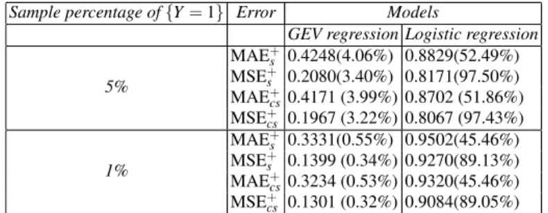
Table 3 reports the MAE and the MSE for each model and for each sample fre-quency of the rare event on the sample (denoted by the subscript “c”) and on the out-of-sample (denoted by the subscript “cs”). In order to evaluate the weights of the errors MSE+and MAE+ on the respective (total) errors MSE and MAE, we compute the ratios(MSE+/MSE)and(MAE+/MAE)weighted by sample relative frequencies of the rare events, equal to 0.05 and 0.01. We report their values be-tween round brackets in Table 3.
From the results reported in Table 3, our proposal exhibits both the MAE and the MSE lower than the respective errors of the logistic regression model for both the sample and control sample and for both the sample percentages of rare events. By comparing the percentages in round brackets, we deduce that for the logistic re-gression model the weights of positive errors are relevant. On the contrary, for our proposal the weights of these positive errorsyi−yˆi>0 are negligible. This means
that the GEV model overcomes the drawback of the logistic regression in the under-estimation of rare events.
Since the errors for the sample and the control sample are similar, the covariates are significant for the default discrimination of both the regression models. This means that both the models are well-explained. Moreover, by comparing the errors for different sample percentages of rare events, our model improves its accuracy by reducing the occurrence probability of the rare event. On the contrary, the logistic regression model shows worse performance. Since the main aim for banks is the
Sample percentage of{Y=1} Error Models
GEV regression Logistic regression
5% MAE+s 0.4248(4.06%) 0.8829(52.49%) MSE+s 0.2080(3.40%) 0.8171(97.50%) MAE+ cs0.4171 (3.99%) 0.8702 (51.86%) MSE+ cs 0.1967 (3.22%) 0.8067 (97.43%) 1% MAE+ s 0.3331(0.55%) 0.9502(45.46%) MSE+ s 0.1399 (0.34%) 0.9270(89.13%) MAE+cs0.3234 (0.53%) 0.9320(45.46%) MSE+cs 0.1301 (0.32%) 0.9084(89.05%)
Table 3 Forecasting accuracy measures of different models over different sample percentage of rare event{Y=1}on the sample (denoted by the subscript “c”) and the out-of-sample (denoted by the subscript “cs”).
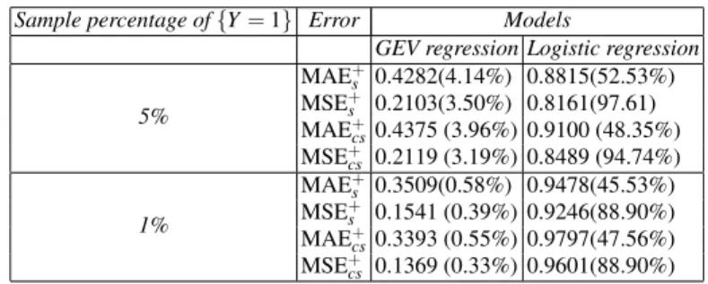
forecasting of default probability, the two models are validated on a subsequent pe-riod. This means that the two models are fitted on data referring the period of time 2004-2008 and the out-of-time predictive accuracy is evaluated on the sample refer-ring to 2009. The sample sizes used in the out-of-time test are reported in Table 2. We compare the predictive accuracy of our model with the logistic one by comput-ing the MAE+and MSE+on the sample (denoted by the subscript “c”) and out-of-time sample (denoted by the subscript “cs”). The results in Table 4 show both the MAE+and MSE+lower than the respective errors of the logistic model. The results obtained from the out-of-time test are coherent with the ones of the out-of-sample
test: in Table 4 the percentages in round brackets exhibit relevant weights of the positive errorsyi−yˆi>0 for the logistic regression and irrelevant positive errors
for our model. Moreover, by comparing the errors for different sample percentages of rare events the logistic model shows a worst performance for lower sample per-centage of rare events: the values of the MAE+and MSE+increase by reducing the percentage of rare events. On the contrary, the GEV model improves its accuracy. From these results the GEV model can be considered a suitable regression model for rare events.
Finally, in order to analyse the robustness of the GEV model we estimate the
coef-Sample percentage of{Y=1} Error Models
GEV regression Logistic regression
5% MAE+ s 0.4282(4.14%) 0.8815(52.53%) MSE+ s 0.2103(3.50%) 0.8161(97.61) MAE+ cs0.4375 (3.96%) 0.9100 (48.35%) MSE+ cs 0.2119 (3.19%) 0.8489 (94.74%) 1% MAE+s 0.3509(0.58%) 0.9478(45.53%) MSE+s 0.1541 (0.39%) 0.9246(88.90%) MAE+cs0.3393 (0.55%) 0.9797(47.56%) MSE+cs 0.1369 (0.33%) 0.9601(88.90%)
Table 4 Forecasting accuracy measures of different models over different sample percentage of rare event{Y=1}on the sample (denoted by the subscript “c”) and the out-of-time (denoted by the subscript “cs”).
ficients of both the regression models on a sample with a given sample percentage of rare events and we evaluate the accuracy on a sample with a different sample percentage of defaulters. By computing the MAE and the MSE on all the SMEs, the errors of our model do not change in comparison with the respective errors above-mentioned on a sample with the same percentage of defaulters1. This means that our model is robust for different sample percentages of defaulters. On the contrary, for the logistic regression models the same errors are significantly different.
Conclusions remarks
In this work we aim at proposing a new GLM regression model with a flexible asymmetric link function for binary response data in rare event studies. At first, we analyse the main drawbacks of the logistic regression model for rare events data. As well known, the GEV distribution is a suitable function for modelling extreme val-ues and rare event data. For this reason we propose the quantile function of the GEV distribution as link function. The GEV model depends on the regression parameters and on the shape parameter of the GEV distribution. Since the score functions do
not have closed-form, we obtain the maximum likelihood estimators by maximizing the log-likelihood function using an iterative algorithm. We specify initial values of parameters for this iterative algorithm and the Fisher information matrix. The main advantage of the GEV model is its excellent performance to identify the rare events. Thanks to this characteristic, the drawback with the logistic regression model in un-derestimating the probability of rare events is overcome.
In order to evaluate the performance of our methodological proposal we apply the GEV model to empirical data on Italian Small Medium Enterprizes (SMEs). Since defaults are events, we model the default probability for Italian SMEs over the years 2005-2009 by considering financial and economic covariates of SMEs. We test this model by comparing the predictive accuracy of our model with the logistic one. The application shows the substantial underestimation of the default probability by applying the logistic regression model. By reducing the sample frequencies of rare events (defaults), the predictive performance of the logistic regression model to identify the rare events becomes worse. On the contrary, the GEV model overcomes the underestimation problem and its accuracy to identify the rare events improves by reducing the sample percentage of rare events. Finally, we shows that the GEV model is a robust model, unlike the logistic regression model.
References
1. Agresti, A. (2002). Categorical Data Analysis. Wiley, New York.
2. Altman E. (1968). Financial ratios, discriminant analysis and the prediction of corporate bankruptcy. Journal of Finance 23(4), 589609.
3. Altman E., Haldeman R., Narayanan P. (1977). ZETA analysis: a new model to identify bankruptcy risk of corporations. Journal of Banking & Finance, 1, 2954.
4. Altman, E., Sabato, G. (2006). Modeling Credit Risk for SMEs: Evidence from the US Mar-ket, ABACUS, 19(6), 716-723 .
5. Ansell, J., Lin, S., Ma Y., Andreeva G. (2009). Experimenting with Modeling Default of Small and Medium Sized Enterprises (SMEs). Credit Scoring and Credit Control XI Conference, August.
6. Barro, R. (2009). Rare Disasters, Asset Prices, and Welfare Costs. American Economic Re-view, vol. 99 (1), 243-64.
7. Basel Committee on Banking Supervision (2004). International convergence of capital mea-surement and capital standards: A revised framework. Bank for International Settlements. Basel, June.
8. Cerved Group (2011). Caratteristiche delle imprese, governance e probabilit di insolvenza. Report. Milan, February.
9. Ciampi F., Gordini N. (2008). Using Economic-Finantial Ratios for Small Enterprize Default Prediction Modeling: an Empirical Analysis. Oxford Business & Economics Conference, Ox-ford.
10. Coles S. G. (2004). An Introduction to Statitical Modelling of Extreme Values. Springer-Verlag, London.
11. Credit Suisse Financial Products (1997). CreditRisk+: A Credit Risk Management Frame-work, Credit Suisse First Boston.
12. Dobson A.J., Barnett A.G. (2008). Introduction to Generalized Linear Models (3rd ed.). Chapman and Hall/CRC, Boca Raton.
13. Dahan E., Mendelson H. (2001). An extreme-value model of concept testing. Management Science, 47, 102116.
14. Danielsson J., de Vries C.G. (1997). Tail index estimation with very high frequency data. Journal of Empirical Finance, 4, 241-257.
15. De Haan L., Cansen D.W., Koedijk K., de Vries C.G. (1994). Safety first portfolio selection, extreme value theory and long run asset risks. In ”Extreme value theory and applications, J. Galambos et al. eds., Kluwer, Dordrecht, 471-487.
16. Dietsch M., Petey J. (2004). Should SME Exposure be treated as Retail or as Corporate Ex-posures? A Comparative Analysis of Default Probabilities and Asset Correlation in French and German SMEs. Journal of Banking and Finance, 28, 773-788.
17. Dowd K. (2002). Measuring Market Risk, John Wiley and Sons, Chichester and New York,. 18. Edmister R. (1972). An Empirical Test of Financial Ratio Analysis for Small Business Failure
Prediction. Journal of Financial and Quantitative Analysis, 7 (2), 1477-1493.
19. Embrechts P., Klppelberg C., Mikosch T. (1997). Modelling Extremal Events for Insurance and Finance, Springer Verlag, Berlin.
20. Embrechts P., S. Resnick, G. Samorodnitsky (1999). Extreme value theory as a risk manage-ment tool. North American Actuarial Journal 3, 30-41.
21. Embrechts P. (2000). Extreme Value Theory: Potential and Limitations as an Integrated Risk Management Tool. Derivatives Use, Trading & Regulation, 6, 449-456.
22. Falk M., Hsler J., Reiss R. (2010). Laws of Small Numbers: Extremes and Rare Events. 3 Edition, Springer, Basel.
23. Finkenstadt B., Rootzen H. (2003). Extreme Values in Finance, Telecommunications, and the Environment. Chapman & Hall, Boca Raton.
24. Fisher R.A., Tippett L.H.C. (1928). Limiting forms of the frequency distributions of the largest or smallest member of a sample. Proceedings of the Cambridge Philosophical Society, 24, 180-190.
25. Frei C., Schr C. (1998). Aprecipitation climatology of the alps from high-resolution rain-gauge observations. Int. J. Climatol., 18, 873-900.
26. Gupton G. M., Finger C. C., Bhatia M. (1997). CreditMetrics. Technical document, Available at http://www.riskmetrics.com/cmtdovv.html.
27. Greene W. H. (2000). Econometric Analysis. Prentice Hall, New York.
28. Hand D.J., Henley W.E. (1997a). Some developments in statistical credit scoring. In: Nakhaeizadeh N, Taylor C (eds) Machine learning and statistics: the interface. Wiley, New York, 221-237.
29. Hand D.J., Henley W.E. (1997b). Statistical classification methods in consumer credit scor-ing: a review. Journal of the Royal Statistical Society, Ser A 160, 523-541.
30. Hand D.J., Niall A. M. (2000). Defining attributes for scorecard construction in credit scoring. Journal of Applied Statistics, 27 (5), 527-540.
31. Hsieh D. A., Manski C.F., McFadden D., (1985). Estimation of Response Probabilities from Augmented Retrospective Observations. Journal of the American Statistical Association, 80 (391), 651-662.
32. Jenkinson A. F. (1955). The frequency distribution of the annual maximum (or minimum) values of meteorological elements. Quarterly Journal of the Royal Meteorological Society, 87, 158-171.
33. King G., Zeng L. (2001). Logistic Regression in Rare Events Data. Political Analysis, 9, 137-163.
34. Kotz S., Nadarajah S. (2000). Extreme Value Distributions. Theory and Applications, Impe-rial Colleg Press, London.
35. Manski C. F., Lerman S. R. (1977). The Estimation of Choice Probabilities from Choice-based Samples. Econometrica 45 (8).
36. McNeil A. J. (1999). Extreme value theory for risk managers. Internal Modelling and CAD II published by RISK Books, 93-113.
37. McCullagh P., Nelder J.A. (1989). Generalized Linear Model, Chapman Hall, New York. 38. McLachlan G. J., Krishnan T. (1997). The EM Algorithm and Extentions. Wiley, New York.
39. Merton R. (1974). On the pricing of corporate debt: The risk structure of interest rates. Journal of Finance, 29, 449-470
40. Prentice R.L. (1986). A case-cohort design for epidemiologic cohort studies and disease pre-vention trials. Biometrika, 66, 403-411.
41. Roberts, S. (2000). Extreme value statistics for novelty detection in biomedical data process-ing. Science, Measurement and Technology, IEE Proceedings, 147, 363-367.
42. Saurina, J., Trucharte C. (2004). The Impact of Basel II on Lending to Small-and Medium-Sized Firms: A Regulatory Policy Assessment Based on Spanish Credit Register Data. Journal of Finance Service Research, 26, 121-144.
43. von Mises R. (1936). La Distribution de la Plus Grande de n Valeurs. In Selected Papers of Richard von Mises, Providence, RI: American Mathematical Society, 2, 271-294.
44. Vozzella P., Gabbi G. (2010). Default and Asset Correlation: An Empirical Study for Italian SMEs. Working Paper.
45. Wilson T. C. (1998). Portfolio credit risk. Economic Policy Review 4, 71-82.
5 Appendix
In this appendix we obtain the score functions and the Fisher information matrix forβ andτof the GEV regression model. The notation used here is defined in the section 3. At first, in order to compute the score functions we consider the following equations ∂li(β,τ,yi) ∂ βj =∂li(π(xi)) ∂ π(xi) ∂ π(xi) ∂ βj ∂li(β,τ,yi) ∂ τ = ∂li(π(xi)) ∂ π(xi) ∂ π(xi) ∂ τ (19)
with j=1,2, ...,kandi=1,2, ...,n. From equations (3) and (5) we obtain that ∂li(π(xi)) ∂ π(xi) = yi π(xi) − 1−yi 1−π(xi) ∂ π(xi) ∂ βj =−xi j(1+τ β0xi)−( 1 τ+1)exp h −(1+τ β0xi)− 1 τ i ∂ π(xi) ∂ τ =−(1+τ β 0x i)− 1 τ 1 τ2ln(1+τ β 0x i)− β0xi τ(1+τ β0xi) exph−(1+τ β0xi)− 1 τ i
Substituting the former results in equations (19), the score functions (6) and (7) are obtained.
The second order partial derivatives of the log-likelihood function with respect to parameters (β,τ) are ∂2li(β,τ,yi) ∂2βj = ∂ 2l i(π(xi)) ∂2π(xi) ∂ π(xi) ∂ βj 2 +∂li(π(xi)) ∂ π(xi) ∂2(π(xi)) ∂2βj ∂2li(β,τ,yi) ∂2τ = ∂2li(π(xi)) ∂2π(xi) ∂ π(xi) ∂ τ 2 +∂li(π(xi)) ∂ π(xi) ∂2(π(xi)) ∂2τ ∂2li(β,τ,yi) ∂ βjβk = ∂ 2li(π(x i)) ∂2π(xi) ∂ π(xi) ∂ βj ∂ π(xi) ∂ βk +∂li(π(xi)) ∂ π(xi) ∂2(π(xi)) ∂ βj∂ βk
∂2li(β,τ,yi) ∂ βjτ = ∂ ∂ βj ∂li(β,τ,yi) ∂ τ where ∂2li(π(xi)) ∂2π(xi) =− yi [π(xi)]2 − 1−yi [1−π(xi)]2 ∂2(π(xi)) ∂2βj =x2i j(1+τ β0xi)− 1 τ−1exp−(1+τ β0xi)− 1 τ τ β0xi−τ 1+τ β0xi ∂2(π(xi)) ∂2τ =π(xi)[−ln(πxi)] 1 τ2ln(1+τ β 0x i)− β0xi τ(1+τ β0x) 2 [−ln(πxi)−1] − −2 τ3ln(1+τ β 0x i) + 2β0xi+τ(β0x)2 τ2(1+τ β0xi) ∂2(π(xi)) ∂ βj∂ βk =xi jxik(1+τ β0x)− 1 τ−1exp−(1+τ β0xi)− 1 τ τ β0xi−τ 1+τ β0xi
The Fisher information is the negative of the expectation of the second derivatives of the log-likelihood with respect to the parametersβandτ
−E ∂2li(β,τ,yi) ∂ βj∂ βk =−∂ π(xi) ∂ βj ∂ π(xi) ∂ βk −E ∂2li(β,τ,yi) ∂2π(xi) =−∂ π(xi) ∂ βj ∂ π(xi) ∂ βk 1 π(xi)[1−π(xi)] −E ∂2li(β,τ,yi) ∂ βj∂ τ =−xi j ln2[π(xi)]π(xi) (1+τ β0x)[1+π(xi)] 1 τ2ln(1+τ β 0x i)− β0xi τ(1+τ β0xi) −E ∂2li(β,τ,yi) ∂2τ =−∂ 2π(x i) ∂2τ 1 π(xi)[1−π(xi)] (20) sinceE ∂li(π(xi)) ∂ π(xi) =0.
By substituting the previous results in the equations (20) the Fisher information matrix is obtained.