High Precision Geoid Determination of Austria Using Heterogeneous Data

High Precision Geoid Determination of

Austria Using Heterogeneous Data

Norbert K¨uhtreiber

Department of Positioning and Navigation, Institute of Geodesy, TU-Graz, Steyrergasse 30, A-8010 Graz, Austria

Abstract. The first Austrian geoid computed by

S¨unkel in 1987, was an astrogeodetic geoid. Later on as a reasonable amount of gravity data was avail-able, a gravimetric geoid has been computed by K¨uhtreiber in 1998. While the astrogeodetic geoid computation in principle provides absolute geoid val-ues, the astrogeodetic method can only provide rel-ative geoid heights. Nevertheless satellite observa-tions (GPS) are used in both cases to fit the geoid. Since heterogeneous measurements (deflections of the vertical, gravity measurements and satellite mea-surements) have different sensibilities in terms of the spectral band of the gravity potential, a combination of all measurements in one computation process us-ing the least squares collocation technique yields best geoid results. The presented Austrian geoid is based on the combination of different data types. The com-bined geoid solution (using deflections of the vertical and gravity anomalies) is influenced by the amount and distribution of the data as well as the weights of the different observations types. Investigations to determine the best possible combination are shown in this work. The precision of the Austrian geoid has improved to the cm-level by combining hetero-geneous data.

1

Data

1.1 Digital Height Model

The Austrian height data used for the present in-vestigation was generated by the Federal Office of Metrology and Surveying. The data is based on grids, with different resolutions determined photogrammet-rically. The grid distance of these grids varies from 30 x 30 m for rough topography to 160 x 160 m in flat areas. From these base models, a digital ter-rain model was derived with the uniform resolution of 1”40625 x 2”34375, or equivalently, 44 m x 49 m,

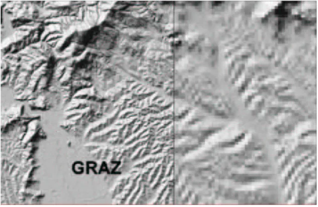
see Graf (1996). The big improvement in the quality of the height model is shown in Fig. (1).

Figure 1. Comparison of the new height model (left side,

resolution 1”40625 x 2”34375) and the old height model (right side, resolution 11”25 x 18”75)

For the neighboring countries, height data in dif-ferent resolution and quality were provided. All height information was used to supplement the Aus-trian height model in the uniform resolution of 1”40625 x 2”34375. A detailed report of the devel-opment of this height model is found in Graf (1996). 1.2 Density

As the gravity signal has a close relation to the den-sity of the underlying masses the denden-sity plays an im-portant role in all geodetic and geophysical process-ing of gravity field quantities. A reasonable density model has to be introduced. Different approaches can be used.

One possible approximation which can be used is a surface density model by assuming that the density of the related grid cells is constant from the surface of the topography down to the crust-mantle bound-ary (Moho). Such a digital surface density model was used for the geoid computation of Austria in 1987. In

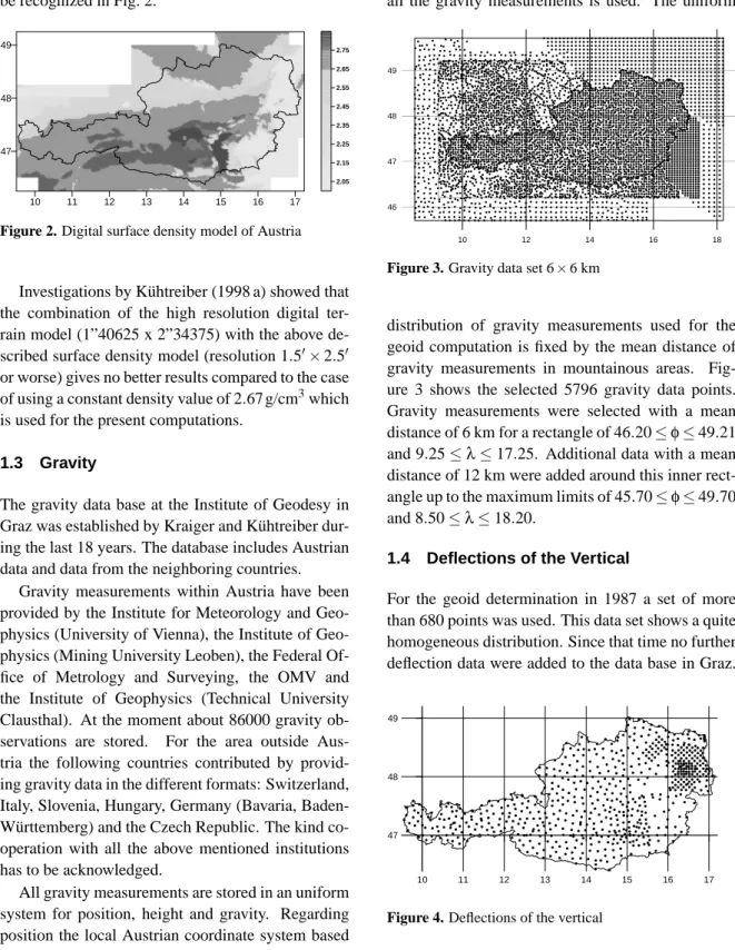
Walach (1987) the history of the mean surface den-sity model of Austria is given. Due to history the resolution of the model is inhomogeneous which can be recognized in Fig. 2. 10 11 12 13 14 15 16 17 47 48 49 2.05 2.15 2.25 2.35 2.45 2.55 2.65 2.75

Figure 2. Digital surface density model of Austria

Investigations by K¨uhtreiber (1998 a) showed that the combination of the high resolution digital ter-rain model (1”40625 x 2”34375) with the above de-scribed surface density model (resolution 1.50×2.50 or worse) gives no better results compared to the case of using a constant density value of 2.67 g/cm3which is used for the present computations.

1.3 Gravity

The gravity data base at the Institute of Geodesy in Graz was established by Kraiger and K¨uhtreiber dur-ing the last 18 years. The database includes Austrian data and data from the neighboring countries.

Gravity measurements within Austria have been provided by the Institute for Meteorology and physics (University of Vienna), the Institute of Geo-physics (Mining University Leoben), the Federal Of-fice of Metrology and Surveying, the OMV and the Institute of Geophysics (Technical University Clausthal). At the moment about 86000 gravity ob-servations are stored. For the area outside Aus-tria the following countries contributed by provid-ing gravity data in the different formats: Switzerland, Italy, Slovenia, Hungary, Germany (Bavaria, Baden-W¨urttemberg) and the Czech Republic. The kind co-operation with all the above mentioned institutions has to be acknowledged.

All gravity measurements are stored in an uniform system for position, height and gravity. Regarding position the local Austrian coordinate system based on the Bessel ellipsoid was chosen. The height sys-tem used is the Austrian orthometric height syssys-tem

based on the tide gage Triest. All gravity measure-ments refer to the system IGSN71.

For the following computations only a subset of all the gravity measurements is used. The uniform

10 12 14 16 18

46 47 48 49

Figure 3. Gravity data set 6×6 km

distribution of gravity measurements used for the geoid computation is fixed by the mean distance of gravity measurements in mountainous areas. Fig-ure 3 shows the selected 5796 gravity data points. Gravity measurements were selected with a mean distance of 6 km for a rectangle of 46.20≤φ≤49.21 and 9.25≤λ≤17.25. Additional data with a mean distance of 12 km were added around this inner rect-angle up to the maximum limits of 45.70≤φ≤49.70 and 8.50≤λ≤18.20.

1.4 Deflections of the Vertical

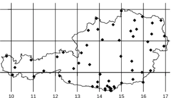
For the geoid determination in 1987 a set of more than 680 points was used. This data set shows a quite homogeneous distribution. Since that time no further deflection data were added to the data base in Graz.

10 11 12 13 14 15 16 17

47 48 49

Figure 4. Deflections of the vertical

the datum of the Military Geographic Institute. Fig-ure 4 shows the data set of deflections used in the following.

1.5 GPS/levelling

Figure 5 shows the distribution of the available GPS/levelling points, which can be used for

scal-10 11 12 13 14 15 16 17

47 48 49

Figure 5. GPS/levelling points

ing as well as for checking the geoid. The points shown are points of the AGREF-net of the Federal Office of Metrology and Surveying. The geocentric coordinates are referred to ITRF94. The orthomet-ric heights refer to UELN98. The distribution of the points is not quite homogeneous as most of the sta-tions are located in the eastern part of Austria. Only few stations are located at the mountainous western part of Austria.

2

Remove-Restore

The geoid computation is done by the well-known remove-restore procedure. The basic idea behind it is to take advantage of the fact that parts of the gravitational potential can be approximated by ex-isting models. The long wavelength part is known through a given earth’s gravitational model which is expressed in terms of a spherical harmonic expan-sion. The short wavelength part is a function of the mass (density) distribution of the topography and can be approximated by a DTM/DDM.

The way the remove-restore technique is applied is the following. In the remove step residual gravity anomalies∆gRESare computed by

∆gRES=∆g−∆gEGM−∆gDT M. (1) The two effects removed from the gravity anomalies

Table 1.Gravity reduction using the standard density of 2.67 g/cm3 and the adapted geopotential model EGM96. Anomalies are given in mgal. Statistics based on 5796 points. (6×6 km set)

min max mean std.dev.

∆gF −154.1 187.2 9.8 ±42.2

∆g_EGM96 −204.3 224.0 −1.1 ±47.6

∆g_iso −72.0 85.4 0.6 ±23.6

∆g are,∆gEGMthe long wavelength part of the

grav-ity anomalies and∆gDT Mthe short to medium wave-length part of the gravity anomalies. By this remove step we gain∆gRES which represent a smooth field with only local-to-regional structures.

Here the adapted EGM96 (Abd-Elmotaal and K¨uhtreiber, 2001) was used to compute the long wavelength part in the remove-restore procedure. For the short to medium wavelengthes a topographic iso-static reduction was performed using the adapted technique and a detailed height model with the res-olution 110025×180075. For the isostatic model an Airy-Heiskanen approach with a standard constant density of 2.67 g/cm3, a normal crustal thickness T of 30 km and a density contrast of 0.4 g/cm3was used. Table 1 shows the statistics for the reduction process. Figure 6 shows the reduced gravity anomaly field.

9 10 11 12 13 14 15 16 17 18 46 47 48 49 -60 -30 0 30 60 90

Figure 6. Gravity Anomalies after removing the short and

long wavelength part of the gravitational potential (contour interval 7.5 mgal).

After the remove-step geoid heights NRESare esti-mated from the residual gravity anomalies∆gRES. In the following the estimation was done by collocation. Details on the used covariance function are given in

sec. 3.

Finally the effects removed are restored again in terms of geoidal heights to NRES

N=NRES+NEGM+δNDT M. (2)

Here δNDT M is nothing else but the indirect effect which takes into account that removing the masses has changed the potential. NEGMis computed using the spherical harmonic expansion of the earth’s grav-itational model.

This technique is commonly applied in local grav-ity field determination. Early computations done by this method are e.g. S¨unkel (1983), Forsberg (1984).

3

Covariance Function

The well-known Tscherning-Rapp covariance func-tion model was used for the following LSC solufunc-tions. The global covariance function of the gravity anoma-lies Cg(P,Q)given by Tscherning and Rapp (1974, p. 29) is written as Cg(P,Q) =A ∞

∑

Q and A, B and s are the model parameters. A closed

expression for (3) is available in (ibid., p. 45). The local covariance function of gravity anoma-lies C(P,Q) given by Tscherning-Rapp can be de-fined as C(P,Q) =A ∞

∑

Modelling the covariance function means in practice fitting the empirically determined covariance func-tion (through its three essential parameters; the vari-ance C◦, the correlation lengthξand the variance of the horizontal gradient G◦H) to the covariance func-tion model. Hence the four parameters A, B, NN and

s are to be determined through this fitting procedure.

A simple fitting of the empirical covariance function was done using COVAXN-Subroutine (Tscherning, 1976).

The essential parameters of the empirical covari-ance parameters for 2489 gravity stations in Austria are 740.47 mgal2for the variance C0and 43.5 km for

the correlation lengthξ. The value for the horizontal gradient G◦Hwas roughly estimated by 100 E2.

For the fixed value B = 24 the following Tscherning-Rapp covariance function model param-eters were fitted: s=0.997065, A=746.002 mgal2 and NN=76. The parameters were used for the as-trogeodetic, the gravimetric as well as the combined geoid solution.

4

Astrogeodetic Solution

The astrogeodetic solution by collocation is based on 659 deflections of the vertical uniformly distributed over Austria (see sec. 1.4). After removing the long

10 12 14 16

46.5 48.5

-1.7 -1.6 -1.5 -1.4 -1.3 -1.2 -1.1 -1.0 -0.9 -0.8

M

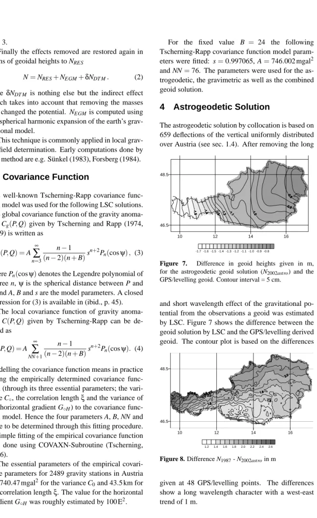
Figure 7. Difference in geoid heights given in m,

for the astrogeodetic geoid solution (N2002astro) and the

GPS/levelling geoid. Contour interval = 5 cm.

and short wavelength effect of the gravitational po-tential from the observations a geoid was estimated by LSC. Figure 7 shows the difference between the geoid solution by LSC and the GPS/levelling derived geoid. The contour plot is based on the differences

10 12 14 16

46.5 48.5

1.2 1.4 1.6 1.8 2.0 2.2 2.4 2.6

M

Figure 8. Difference N1987- N2002astroin m

given at 48 GPS/levelling points. The differences show a long wavelength character with a west-east trend of 1 m.

After the new astrogeodetic solution (N2002astro)

has been fitted to all GPS/levelling points using col-location the new astrogeodetic solution is compared to the Austrian geoid solution of 1987 (N1987) which

is based on the same data set of deflections (see Fig. 8). The big offset of 1.2 to 2.6 m can be ex-plained by the fact that the solution of 1987 has been scaled by Doppler/levelling points, which provide an accuracy of about 1 to 2 m only. Besides the big north-south trend we notice short wavelength vari-ations which can be explained by the better height information used in the new solution.

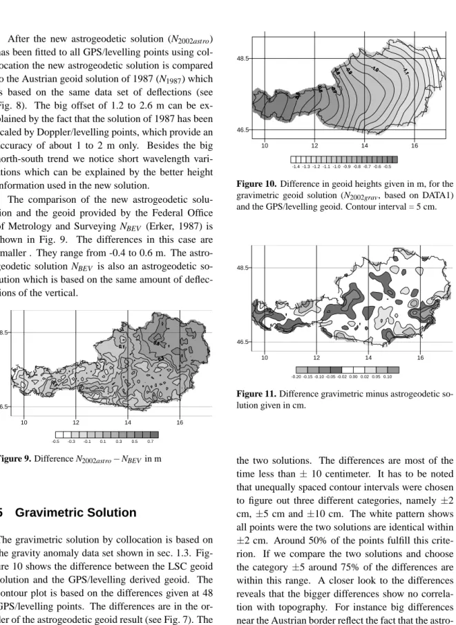
The comparison of the new astrogeodetic solu-tion and the geoid provided by the Federal Office of Metrology and Surveying NBEV (Erker, 1987) is shown in Fig. 9. The differences in this case are smaller . They range from -0.4 to 0.6 m. The astro-geodetic solution NBEV is also an astrogeodetic so-lution which is based on the same amount of deflec-tions of the vertical.

10 12 14 16

46.5 48.5

-0.5 -0.3 -0.1 0.1 0.3 0.5 0.7

M

Figure 9. Difference N2002astro−NBEV in m

5

Gravimetric Solution

The gravimetric solution by collocation is based on the gravity anomaly data set shown in sec. 1.3. Fig-ure 10 shows the difference between the LSC geoid solution and the GPS/levelling derived geoid. The contour plot is based on the differences given at 48 GPS/levelling points. The differences are in the or-der of the astrogeodetic geoid result (see Fig. 7). The differences show a high order polynomial trend with a west-east gradient of about 0.8 m.

Of particular interest is how the new gravimetric solution N2002gravfits the new astrogeodetic solution

N2002astro. Figure 11 shows the difference between

10 12 14 16

46.5 48.5

-1.4 -1.3 -1.2 -1.1 -1.0 -0.9 -0.8 -0.7 -0.6 -0.5

M

Figure 10. Difference in geoid heights given in m, for the

gravimetric geoid solution (N2002grav, based on DATA1)

and the GPS/levelling geoid. Contour interval = 5 cm.

10 12 14 16

46.5 48.5

-0.20 -0.15 -0.10 -0.05 -0.02 0.00 0.02 0.05 0.10

M

Figure 11. Difference gravimetric minus astrogeodetic

so-lution given in cm.

the two solutions. The differences are most of the time less than±10 centimeter. It has to be noted that unequally spaced contour intervals were chosen to figure out three different categories, namely±2 cm,±5 cm and±10 cm. The white pattern shows all points were the two solutions are identical within

±2 cm. Around 50% of the points fulfill this crite-rion. If we compare the two solutions and choose the category±5 around 75% of the differences are within this range. A closer look to the differences reveals that the bigger differences show no correla-tion with topography. For instance big differences near the Austrian border reflect the fact that the astro-geodetic solution is a local solution based on deflec-tions points inside Austria only, while the gravimet-ric solution was computed on a more regional basis. The biggest difference is located in the eastern part of Austria.

10 12 14 16 46.5

48.5

-0.04 -0.01 0.00 0.01 0.04

M

Figure 12. Difference astrogeodetic minus gravimetric

so-lution given in cm.

In order to get an explanation for the discrepan-cies between the two solutions, the difference is plot-ted once again in combination with the used set of deflection points (cf. Fig. 12). The light grey pat-tern is used for areas where the difference between the gravimetric and astrogeodetic solution is within

±1 cm. In the north-eastern part of Austria a larger area exists which fulfills the criterion. Within this area we recognize the densest coverage with deflec-tion points. In contradictory the dark grey parts mark regions where the difference between the two solu-tions are bigger than -4 cm. In the south-east of Aus-tria (east part of Styria) the difference is bigger than -15 cm. In this area only a very sparse distribution of deflection points can be recognized. A similar con-clusion holds for the areas with a difference bigger than 4 cm (middle grey pattern). Figure 12 shows clearly that the difference depends on the distribution of the deflection points. The more homogeneous and dense the distribution of deflection points the better the two solutions fit. Of course differences are also dependent on the smoothness of the residual gravita-tional potential. Therefore we can draw the following conclusion. In order to get a precise geoid solution, the residual gravitational field should be as smooth as possible and the used measurements should homoge-neously cover the region.

6

Combined Solution

The first combined solution was done by K¨uhtreiber (1999). This combination of the gravimetric and as-trogeodetic geoid was done by computing a simple arithmetic mean of the astrogeodetic and the gravi-metric solution. In order to take advantage of

collo-cation for combining gravity anomalies and deflec-tions of the vertical in one estimation process in-vestigations concerning the weighting of the gravity anomalies versus the deflections of the vertical are needed.

An important point concerning a reasonable com-bination of deflections of the vertical and gravity anomalies in a collocation process is the definition of the error variances for the different data types. A case study was performed by the following ap-proach. Geoid heights were computed by a combina-tion of defleccombina-tions of the vertical and gravity anoma-lies. Three different cases, each with a different error variance of∆g, but all with equal error variances for

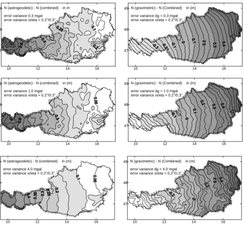
the deflections of the vertical, are considered. Each of the combined solution is compared to the pure as-trogeodetic or pure gravimetric geoid solution (see Fig. 13).

Let us consider the starting configuration. The er-ror variance of∆g was given as 0.3 mgal while the

error variances of the deflectionsξandηwere given as 0.200 and 0.300respectively. Comparing the com-bined solution with the astrogeodetic solution shows more or less a big west-east trend with regions which don’t fit the trend at all (e.g. eastern part of Aus-tria). The difference between the combined solution and the gravimetric solution is a pure trend, no devi-ation from the trend is visible. The conclusions we can draw from the first pair of plots in Fig. 13 are:

- the error variance of 0.3 mgal for the gravity anomalies is too small. Hence the deflections of the vertical don’t contribute to the solution on a local ba-sis

- big discrepancies between the astrogeodetic and combined solutions appear in regions with sparse dis-tributed deflections in all three cases

Increasing the error variance of the gravity anoma-lies should down-weight the part of the gravity anomalies in the combined solution, while the deflec-tions should contribute more to the solution with the same error variances. We would expect that the dif-ference between the astrogeodetic and the combined solution becomes more a pure trend, while the differ-ence between the gravimetric and the combined so-lution becomes more irregular. The second and third pairs of plots in Fig. 13 prove this consideration.

The poor results of the astrogeodetic solution in the east of Styria exists in all solutions. Even a very high weight of the deflections relative to the gravity

10 12 14 16 47

48

49 N (astrogeodetic) - N (combined) in m error variance 0.3 mgal

error variance xi/eta = 0.2"/0.3"

10 12 14 16

47 48

49 N (gravimetric) - N (Combined) in (m) error variance dg = 0.3 mgal error variance xi/eta = 0.2"/0.3"

10 12 14 16

47 48

49 N (astrogeodetic) - N (combined) in (m) error variance 1.0 mgal

error variance xi/eta = 0.2"/0.3"

10 12 14 16

47 48

49 N (gravimetric) - N (Combined) in (m) error variance dg = 1.0 mgal error variance xi/eta = 0.2"/0.3"

10 12 14 16

47 48

49 N (astrogeodetic) - N (combined) in (m) error variance 4.0 mgal

error variance xi/eta = 0.2"/0.3"

10 12 14 16

47 48

49 N (gravimetric) - N (Combined) in (m) error variance dg = 4.0 mgal error variance xi/eta = 0.2"/0.3"

M

Figure 13. Changing the error variance of the gravity anomalies in the combined solution and comparing the solution to the

astrogeodetic and gravimetric solution.

anomalies preserves the structure of the gravimetric geoid solution to some extent. This is clear as the deflections of the vertical are too sparse in this area to contribute to the combined solution.

10 12 14 16

46.5 48.5

-1.0 -0.9 -0.8 -0.7

M

Figure 14. Difference in geoid heights given in m, for

the combined geoid solution and the GPS/levelling geoid. Contour interval = 5 cm.

As a conclusion of this study, the error variances of the gravity anomalies and the deflections of the vertical were chosen as 1.5 mgal for∆g and 0.2”, 0.3”

forξ,η, respectively.

Finally fig. 14 shows the difference between the combined LSC geoid solution and the GPS/levelling derived geoid. The contour plot is based on the ferences given at 48 GPS/levelling points. The dif-ferences show by far the smoothest behaviour and the smallest range.

7

Restore and Scaling

The effect of the adapted EGM96 and the topographic-isostatic model were restored. The re-sulting geoid heights were scaled to 12 GPS/levelling points, while 38 GPS/levelling points were used for an external check. Table 2 shows the statistics of this check.

Table 2. Differences between the geoid solu-tions N2002astro, N2002gravi and N2002 to N from

GPS/Levelling given in cm. Statistics based on 38 external checking points

min max std.dev.

N2002astro −12.7 10.6 ±4.4

N2002gravi −7.4 9.4 ±3.8

N2002 −7.2 7.5 ±3.4

8

Conclusions

With the help of the adapted technique for estimation of the influence of the short and longwavelength part of the gravity field and the LSC approach combin-ing gravity anomalies and deflections of the vertical a high precision geoid for Austria was estimated. The major achievements of the solution are:

- an excellent agreement of the astrogeodetic and gravimetric geoid solution

- a centimeter accuracy of the geoid solution as result of the combined solution

- a considerable improvement compared to the old solution in the eastern part of Styria and all areas in the vicinity to the Austrian border

- an external check with GPS/levelling points with a standard deviation of±3.4 cm for the differences

- a practical tool for providing levelling heights through GPS measurement.

References

Abd-Elmotaal, H. and K¨uhtreiber, N. (2001) Precise Geoid Computation Employing Adapted Refer-ence Field, Seismic Moho Information and Vari-able Density Anomaly, Presented at the Scien-tific Assembly of the International Association of Geodesy IAG 2001, Budapest, Hungary, Septem-ber 2–8, 2001.

Erker, E., (1987) The Austrian Geoid - Local Geoid Determination Using Modified Conserva-tive Algorithms, In: Gravity Field in Austria, Geod¨atische Arbeiten ¨Ostereichs f¨ur die Interna-tionale Erdmessung, Graz,4.

Forsberg, R. (1984) A Study of Terrain Reduc-tions, Density Anomalies and Geophysical Inver-sion Methods in Gravity Field Modelling, Depart-ment of Geodetic Science, Ohio State University,

Columbus, Ohio,355.

Graf, J. (1996) Das digitale Gel¨andemodell f¨ur Geoidberechnungen und Schwerereduktionen in

¨

Osterreich, Proceedings of the 7th Interna-tional Meeting on Alpine Gravimetry, Vienna,

¨

Osterreichische Beitr¨age zu Meteorologie und Geophysik,14, 121–136.

K¨uhtreiber, N. (1998 a) Precise Geoid Determina-tion Using a Density VariaDetermina-tion Model,Physics and Chemistry of the Earth,23 (1), 59–63.

K¨uhtreiber, N. (1998 b) Improved Gravimetric Geoid AGG97 of Austria, In Forsberg, R., Feissel, M. and Dietrich, R., eds., Geodesy on the Move: Gravity, Geoid, Geodynamics and Antarctica, IAG Symposia, 119, Rio de Janeiro, Brazil,

September 3–9, 1997, 306–311.

K¨uhtreiber, N. (1999) Combining Gravity Anomalies and Deflections of the Vertical for a Precise Aus-trian Geoid,Bollettino di Geofisica teorica ed ap-plicata,40, 545–553.

S¨unkel, H. (1983) Geoidbestimmung, Berechnungen an der TU Graz, 2. Teil, In Lichtenegger, H., Rinner, K. and S¨unkel, H., eds., Das Geoid in

¨

Osterreich, Geod¨atische Arbeiten ¨Osterreichs f¨ur die Internationale Erdmessung,3, 125–143.

S¨unkel, H., Bartelme, N., Fuchs, H., Hanafy, M., Schuh, W., Wieser, M., (1987) The Gravity Field in Austria, In: Gravity Field in Austria, Geod¨atische Arbeiten ¨Ostereichs f¨ur die Interna-tionale Erdmessung, Graz,4.

Tscherning, C.C. (1976) Implementation of Algol-Procedures for Covariance Computation on the RC 4000-Computer, The Danish Geodetic Insti-tute,12.

Tscherning, C.C. and Rapp, R.H. (1974) Closed Covariance Expressions for Gravity Anomalies, Geoid Undulations, and Deflections of the Verti-cal Implied by Anomaly Degree Variance Models,

Department of Geodetic Science, The Ohio State University, Columbus, Ohio,208.

Walach, G. (1987) A Digital Model of Surface Rock Densities of Austria and the Alpine Realm,

In: Gravity Field in Austria, Geod¨atische Ar-beiten ¨Ostereichs f¨ur die Internationale Erdmes-sung, Graz,4.