Unemployment Dynamics and Endogenous
Unemployment Insurance Extensions
∗
W. Similan Rujiwattanapong
†May 1, 2019
Abstract
This paper investigates the impact of endogenous unemployment insur-ance (UI) extensions on the dynamics of unemployment and its duration structure in the US. Using a search and matching model with worker het-erogeneity, I allow for the maximum UI duration to depend on unemploy-ment and for UI benefits to depend on worker characteristics. UI extensions have a large effect on long-term unemployment during the Great Recession via job search responses and a moderate effect on total unemployment via job separations. Disregarding rational expectations about the timing of UI extensions implies an overestimation of the unemployment rate by over 2 percentage points.
JEL Classification.E24, E32, J24, J64, J65.
Keywords.Business cycles, long-term unemployment, unemployment insurance, unemployment duration, rational expectations
∗I am indebted to Morten Ravn for invaluable guidance and support, and to Fabien
Postel-Vinay and Vincent Sterk for very helpful discussions and suggestions. I also want to thank Wei Cui, Gregor Jarosch, Fatih Karahan, Jeremy Lise, Kurt Mitman, Suphanit Piyapromdee, Shouy-ong Shi, Ludo Visschers and Randall Wright as well as seminar participants at Aarhus University, Bank of Thailand, University of Bath, Birkbeck University of London, GRIPS, Hitotsubashi Uni-versity, University of Konstanz, Queen Mary University of London, University of Tokyo, UCL, Bristol Search and Matching Workshop, and Nordic summer symposium in Macroeconomics for helpful comments and conversations. This paper was previously circulated as “Long-term Unem-ployment Dynamics and UnemUnem-ployment Insurance Extensions”.
†Aarhus University and Centre for Macroeconomics. Mailing Address: Department of
Eco-nomics, Aarhus BSS, Aarhus University, Fuglesangs Alle 4, Aarhus V, 8210, Denmark. Email:
1
Introduction/Motivation
From the onset of the Great Recession, the US labour market exhibits dynam-ics never seen before in previous recessions. Underlying persistently high unem-ployment is an unprecedented rise in long-term unemunem-ployment (represented by those whose unemployment duration is greater than 6 months) as seen in Figure
1. Long-term unemployment had always been below a quarter of total unemploy-ment apart from two occasions: the Great Recession when it represented almost half of the total unemployment population and the early 1980s recession where it represented a quarter of total unemployment.1
This paper investigates the impact of endogenous unemployment insurance (UI) extensions on the dynamics of unemployment and its duration structure un-der rational expectations using a search and matching model in general equilib-rium. Whilst the analysis applies to cyclical fluctuations in general, the focus of the paper is on the Great Recession, the period during which UI eligible unem-ployed workers could receive benefits for a maximum of 99 weeks (whereas the standard maximum UI duration is 26 weeks) as depicted in Figure 2 From the same figure, it can be seen that the maximum UI duration has been extended in every recession since late 1950s, and its generosity, measured by weeks of maxi-mum UI duration, has been increasing over time (except for one extension in the early 1980s). There are primarily two types of UI extensions in the US: (1) auto-matic UI extensions that are in the federal laws since 1970s and are triggered by the state (insured) unemployment rate, and (2) discretionary UI extensions that are issued specifically during recessions.2 It is the first type that endogenises UI extensions and makes them countercyclical.3
Based on this countercyclical UI system, I extend the standard search and matching model to incorporate unemployment-dependent UI extensions, variable search intensity, endogenous separations, on-the-job search, and worker’s
hetero-1Abraham, Haltiwanger, Sandusky, and Spletzer (2016) find that long-term unemployed work-ers face worse labour market outcomes in terms of re-employment probabilities and subsequent earnings even when controlled for individual heterogeneity.
2The automatic extensions are called extended benefits (EB) whilst the ad-hoc extensions are under different names. For example, in 1958, the programme was called Temporary Unemploy-ment Compensation Act (TUC), and in 1961, it was Temporary UnemployUnemploy-ment Extended Com-pensation Act (TEUC). From 1991 onwards, the discretionary extensions have been under the name Emergency Unemployment Compensation (EUC).
3We can also see from Figure2that both the automatic and discretionary extensions have been increasing in their generosity and that they are a feature of every recession since late 1950s.
geneity in terms of productivity and benefit level. The job search decision of a worker depends not only on their UI status, benefit level, and individual produc-tivity but also on the aggregate producproduc-tivity and the unemployment rate which determine when and for how long UI extensions will occur.
Many empirical studies have documented how the labour market outcomes of unemployed workers can differ with respect to their UI status. These dif-ferences come in many forms including their unemployment duration and unem-ployment exit rate (Moffitt and Nicholson (1982), Moffitt (1985), Katz and Meyer (1990), Meyer (1990), Card and Levine (2000)), job search intensity (Krueger and Mueller (2010, 2011)), and consumption (Gruber (1997)). Katz and Meyer (1990) find a large fraction of UI recipients expect to be recalled and represent over half of the unemployment duration in the sample. This is related to Fujita and Moscarini (2015) who show that the recall rate rises during recessions. I pro-vide further empirical epro-vidence that insured unemployed workers have a lower unemployment exit rate than the uninsured and this gap widened during the Great Recession when UI extensions took place.
There is a large literature studying the effects of the recent UI extensions on the unemployment exit rate and total unemployment during the Great Recession. Empirical studies include (but not limited to) Farber and Valletta (2011), Fujita (2011), Valletta and Kuang (2010), Aaronson, Mazumder, and Schechter (2010), Mazumder (2011), Rothstein (2011), Barnichon and Figura (2014), and Hage-dorn, Karahan, Manovskii, and Mitman (2019). Most of these studies focus on the microeconomic effect of the UI extensions, namely, the impact on the prob-ability of exiting unemployment or on the job search efforts of the unemployed. They found a small but significant impact of UI extensions. A notable exception is Hagedorn et al. (2019) as they take into account the response of job creation to benefit extensions and find a larger effect on unemployment.
A benefit of using a general equilibrium model is that I can distinguish be-tween the microeconomic and general equilibrium effects of UI extensions on unemployment. I find that UI extensions contribute to a 0.9-1.8 percentage point (pp) increase in unemployment under the micro effect during the Great Recession which is consistent with existing empirical estimates.4 I find that the general
equi-4Existing estimates are in the range of 0.1-1.8pp. Fujita (2011) finds the UI extensions con-tribute to a 0.8-1.8pp increase in the unemployment rate during the Great Recession. Aaronson et al. (2010)’s estimates are between 0.5-1.25pp. Valetta and Kuang (2010)’s estimate is 0.4pp. Rothstein (2011)’s estimates are between 0.1-0.5pp.
librium effect of UI, where worker-firm match formation/separation decisions are taken into account, is larger and similar to results from Hagedorn et al. (2019). In this paper, however, the additional effect is from the match separation margin.5
Studies on the effects of UI extensions in general equilibrium are conducted by Mitman and Rabinovich (2014) on jobless recoveries, Faig, Zhang and Zhang (2016) on the volatility of unemployment and vacancies, and Nakajima (2012) whose focus is on the Great Recession.6 The model in this paper is most similar to that in Mitman and Rabinovich (2014) and departs from theirs in two crucial aspects: (1) the endogeneity of UI extensions and (2) the heterogeneous job find-ing rates.
In their model, UI extensions are exogenous and assumed to last forever (i.e., agents have adaptive expectations). In my model, I assume that UI extensions are totally systematic, and agents have rational expectations regarding the tim-ing and the length of these extensions which are governed by the unemployment rate, just like in the US economy. Agents in my model would therefore respond less strongly to UI extensions than in their model, in terms of both the job search intensity and the decision to form or dissolve a match. Additionally, workers in my model optimally choose their job search intensity whilst job search is fixed in their model. Therefore, unemployed workers in my model have heterogeneous job finding rates according to their UI status and benefit level whilst there is a sin-gle job finding rate in their model. I show in the empirical section that insured and uninsured unemployed workers do have different job finding rates. Heterogeneity in the job finding rates is crucial in explaining the unemployment duration struc-ture in the US labour market. Wiczer (2015) shows that a single job finding rate implies an average unemployment duration and long-term unemployment that are just over half of what we observed in the data. This point regarding an inadequacy of a single job finding rate is key to the results in this paper.7
This paper also relates to the literature on the incidence of long-term unemploy-ment and worker heterogeneity. Ahn and Hamilton (2019) use a non-linear state space model to uncover the unobserved heterogeneity of workers’ unemployment
5Henceforth, I define job separations as employment-to-unemployment transtions.
6Nakajima (2012) studies an economy with transitional dynamics and finds that the UI exten-sions contribute to a 1.4pp increase in the unemployment rate.
7In Rujiwattanapong (2017), I show that a single job finding rate for insured unemployed workers hardly affects the distribution of unemployment durations. In this paper, I allow for the job finding rates of insured unemployed workers to vary with the benefit level and individual-specific productivity.
exit rate. Worker heterogeneity is the focus of Hornstein (2012) in accounting for unemployment dynamics with different durations. Ravn and Sterk (2017) con-sider the difference in unemployment exit rates together with incomplete mar-kets and price rigidities to study the amplification mechanism on unemployment. Carrillo-Tudela and Visschers (2014) study the role of unemployed workers’ oc-cupational mobility on the fluctuations of unemployment and its duration over business cycles. Kroft, Lange, Notowidigdo, and Katz (2016) analyse the impact of a genuine duration dependence in unemployment exit rate on the rise of long-term unemployment. They find little account for the observable characteristics of workers. Ahn (2016) extends Ahn and Hamilton (2019) to incorporate observable characteristics of the workers (but not their UI status).
My paper considers a degree of observed and unobserved worker heterogeneity where the former comes from the UI status and benefit level, and the latter is from the worker’s productivity, all of which affect the job finding rate. I also estimate the same model in Ahn and Hamilton (2019) using Maximum Likelihood and show that their interpretation of unobserved heterogeneity is related to the UI sta-tus in my model since insured unemployed workers have a lower unemployment exit rate. I find that worker productivity does not matter much once the UI status and benefit level are taken into account.
The main contributions of this paper are twofold. First, it quantifies the mi-croeconomic and general equilibrium effects of UI extensions on unemployment and its duration structure. Second, it demonstrates the importance of rational ex-pectations regarding the timings of endogenous UI extensions. The framework is useful for policy experiments to study the mechanisms through which UI exten-sions affect the aggregate labour market.
To preview the results, I find that UI extensions account for 10-30 percent of the rise on unemployment during the Great Recession, but the UI effect is non-linear and of a smaller magnitude in other recessions. The main mechanism through which UI extensions impact unemployment is the job separation margin whereas the job search behaviour is most important for long-term unemployment. I show that a failure to take into account rational expectations about the timing of UI extensions implies an overestimation of unemployment by more than 2pp.
The paper is organised as follows. Section 2 discusses some motivating data on UI extensions and long-term unemployment during the Great Recession. Section 3 describes the model. Section 4 discusses the calibration exercise. Section 5
analyses the results under the baseline model and counterfactual experiments. Section 6 concludes.
2
Empirical Evidence
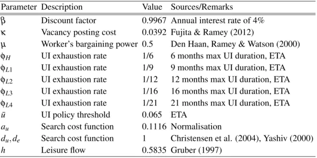
I examine the empirical evidence that (1) workers currently receiving UI bene-fits are less likely to find a job than workers without UI, and that (2) this gap be-tween insured and uninsured workers’ job finding rates was more pronounced dur-ing the Great Recession. These finddur-ings are important for explaindur-ing the surge in long-term unemployment. I study the transition rates from unemployment to em-ployment, unemployment and out-of-labour-force (OLF) (namely UE, UU, and UOLF rates respectively), as well as the distributions of unemployment duration between 2006 and 2014 according to the UI status and several observable charac-teristics of unemployed workers including age, education, gender, industry, occu-pation, reasons for unemployment, and recall expectation. They are constructed from the CPS Basic Monthly Data and CPS Displaced Worker, Employee Tenure, and Occupational Mobility Supplement.8
Job findings Table 1 shows that the job finding rate of current UI recipients
is generally smaller than that of non-UI recipients, and this gap became larger during the Great Recession. In January 2008, when there was no UI extensions, unemployed workers with and without UI found a job at rate 21 percent and 28 percent respectively, whilst in January 2010, when the maximum UI duration was 99 weeks, the job finding rate of insured unemployed workers fell dramatically to 7 percent, 11pp smaller than that of the uninsured unemployed. The findings remain the same when I control for other observable worker characteristics as shown in TableA.1of Appendix A.9
To stay unemployed or to exit the labour force? Accompanying the drop in
job findings during the Great Recession are an increase in the UU rate and little
8I consider workers whose age is 16 years or older. Since the workers’ UI history is only surveyed when the supplement takes place (every two years), I obtain the transition rates by merging the January supplement data with the basic monthly data for the following February. Transition rates are calculated as a fraction of unemployed workers conditioned on their UI status (i.e., whether they are currently receiving UI benefits or not) and possibly other characteristics moving into either employment, unemployment, or OLF in the following month.
9Specifically, insured unemployed workers had a lower job finding rate than uninsured unem-ployed workers in most subgroups in 2008 and in all subgroups in 2010. The job finding rates from 2008 to 2010 for current UI recipients in most subgroups fell by a larger magnitude than for non-UI recipients.
change in the UOLF rate. This is the case regardless of the UI status. Table1
shows that from 2008 to 2010 the UU rate increased by 16pp for workers with UI and by 12pp for workers without UI. At the same time, Table1shows that the fall in the UOLF rate was only 2(3)pp for the (un)insured unemployed. This suggests that UI extensions do not significantly affect the labour force exit rate.10 The same results apply when I condition on other observable worker characteristics as shown in TableA.2andA.3of Appendix A.
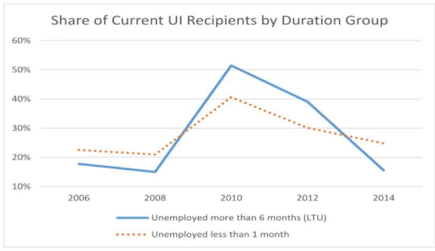
Distribution of unemployment duration The share of long-term unemployed
workers who were current UI recipients rose substantially from 15 percent to 51 percent between 2008 and 2010 as shown in Figure3. This large increase in the share of current UI recipients during the Great Recession is a prominent feature in all subgroups considered as shown in TableA.4 of Appendix A. In Figure3, I contrast this with the shares of insured workers amongst the newly unemployed that did not increase as much.
These empirical findings motivate the model in the next section to feature a de-gree of worker heterogeneity and endogenous job search intensity which together imply heterogeneous job finding probabilities.
3
Model
I present a search and matching model `a la Pissarides (2000) with endogenous separations, variable job search intensity, and on-the-job search. On top of this, I allow for the maximum UI duration to depend on the unemployment rate. Work-ers differ in terms of UI status, benefit level, and labour productivity. Only the last attribute is permanent. These differences not only affect how hard workers search for jobs, but also how likely worker-firm matches are formed and sepa-rated. Workers with higher outside options, e.g. those with higher (potential) UI benefits, tend to exit unemployment more slowly and are more likely to quit. I begin this section by specifying technology and preferences of workers and firms as well as the UI duration policy and UI eligibility. I then discuss wage determi-nation, and finally I present the equilibrium conditions.
10For simplicity, the model I present in the following section will therefore not feature the labour force participation margin. Barnichon and Figura (2014) also find that UI extensions did not affect the labour force participation rate in the past 35 years.
3.1
Technology and Preferences
Time is discrete and runs forever. There are two types of agents in the econ-omy: a continuum of workers of measure one and a large measure of firms. Workers have either high or low productivity (type H or L). A match consists of one worker and one firm whose output depends on the aggregate productiv-ity (z), its match-specific productivity (m), and type-iworker’s productivity (ηi). Specifically, yit(m) =zt×m×ηi ;i∈ {H,L}. The price of output yit(m) is normalised to one. The aggregate productivity z has an AR(1) representation: lnzt = ρzlnzt−1+εt where εt ∼ N(0,σz2) is the only exogenous shock in the
model. The match-specific productivity m is drawn at the start of every new worker-firm match from a distribution F(m). A given match gets to keep its match qualitymto the next period with probability 1−λ, otherwise it redraws a
newmfromF(m)for its production next period.ηiis type-iworker’s productivity whereηL<ηH≡1. A worker’s productivity is permanent.
With respect to preferences, both workers and firms are infinitely-lived and risk-neutral. They discount future flows by the same factor β ∈(0,1).
Work-ers are either employed (e), insured unemployed (U I), or uninsured unemployed (UU). They exert job search effort s at the cost of νe(s) when employed, and at the cost νu(s) when unemployed regardless of their UI status. These search cost functionsνe(.) andνu(.) are strictly increasing and convex. During unem-ployment, workers’ job search intensity may vary depending on their UI status, benefit level, and both aggregate and individual productivities, whilst during em-ployment, it depends on their match quality and both aggregate and individual productivities.11 For employment status j∈ {e,u}, a worker’s period utility flow isci−νj(s)whereciis type-iworker’s consumption:
cit =
wit(m,m˜) if employed at match qualitym h+bi(m˜) if insured unemployed
h if uninsured unemployed
11Unemployment duration could be an important factor since the insured unemployed closer to benefit exhaustion (or with a higher rate of exhaustion) search harder for jobs. I allowed for unemployment duration to be an individual state variable and find that the results remain largely the same. This is due to the risk neutrality assumption. If workers are instead risk averse, their job search response to unemployment duration is expected to be stronger but such analysis is beyond the scope of the paper.
wherewi(m,m˜)is the wage of type-iworker that depends onm, the current match quality, and ˜m, the match quality in her most recent employment. hcan be inter-preted as home production or leisure flow during unemployment.bi(m˜)is the UI benefit of type-iworker with match quality ˜min her most recent employment. I describe the UI system and the wage determination in the next subsections.
Firms are either matched with a worker or unmatched. Matched firms sell output, pay negotiated wage to their workers, and pay lump-sum taxτ to finance
the UI payment. A match is exogenously separated at rateδ, and an endogenous
separation can occur when the value of a worker being matched to a firm or vice versa is negative. When firms are unmatched with a worker, they post a vacancy at costκ and cannot direct their posting to a specific type of workers.
3.1.1 UI Duration Policy and UI Eligibility
UI Duration The maximum UI duration is captured by the variable φ(ut).
Specifically, insured unemployed workers exhaust their UI benefits at the rate
φ(ut) ≡ φL1{ut≥u¯}+φH1{ut<u¯}
where φL <φH implying that the UI exhaustion rate is a decreasing function of the unemployment rateut in the economy.12 Since the inverse ofφ(ut)is the ex-pected duration of receiving UI benefits, a fall in the rate implies a UI extension. This is set to mimic the rules for UI extensions in the US where they depend on the state unemployment rate (above which UI extensions are triggered).13 I can capture the observed increase in the generosity of UI extensions in the US by lowering in the value thatφL takes. Economic agents can predict whether a UI extension will be triggered/terminated next period by keeping track of unemploy-ment and relevant distributions.
UI Eligibility Upon losing a job, employed workers become uninsured at rate
1−ψ. This reflects how some unemployed workers do not take up UI benefits. On
top of this, insured unemployed workers lose UI eligibility after an unproductive meeting with a firm at rateξ to reflect how UI recipients’ job search is monitored.
12This stochastic UI exhaustion is first used in Fredericksson and Holmlund (2001). Mitman and Rabinovich (2014), Faig, Zhang and Zhang (2016), and Rujiwattanapong (2017) treat this rate to be state-dependent.
13Specifically, during normal times (u
t<u¯), the UI exhaustion rate isφH which is set to imply
a standard UI duration of 26 weeks. When the unemployment rate is high and above ¯u(often in recessions), insured unemployed workers exhaust the benefits at a slower rateφL.
UI payment is financed each period by lump-sum tax (τ) levied on matched
firms:
τ(1−u) =
∑
i∈{H,L}
∑
m˜uU Ii (m˜)bi(m˜) (1)
where uU Ii (m˜) is the number of type-i insured unemployed workers whose UI benefit isbi(m˜).
3.1.2 Search and Matching
Workers and unmatched firms meet via a meeting functionM(s,v)wheresis the aggregate search intensity, andvis the number of job vacancies. The meeting functionM(., .)has constant returns to scale and is strictly increasing and concave in its arguments. Market tightness can be defined asθ ≡v/s. The conditional job
finding probability per unit of search is Ms =M(1,θ); therefore, the conditional
job finding probability of type-iworker with employment status jissijM(1,θ)≡
pij(θ).14 Analogously, the probability that a firm meets a worker is Mv ≡q(θ).
3.1.3 Timing
1) Given (ut,zt), production takes place, and UI duration policyφ(ut)is set. 2) Workers choose job search effort. 3) Current matches draw a newmat rateλ. 4)
Workers and unmatched firms meet. 5) Aggregate productivityzt+1 next period
is realised. 6) Matches/meetings dissolve. 7)uU I lose UI eligibility at rateφ(ut) if not meeting a firm, or at rateφ(ut) + 1−φ(ut)
ξ if a meeting has occurred.
8) Unemploymentut+1for next period is realised.
3.1.4 Workers’ Value Functions
I first define the set of state variables asω≡ {z,u,ui,uU Ii (m˜),uUUi ,ei(m);∀m,∀m˜ andi∈ {H,L}} where ui is the number of type-i unemployed workers, uU Ii (m˜) is the
number of type-iinsured unemployed workers whose match quality in their most recent employment was ˜m, uUUi is the number of type-i uninsured unemployed workers, andei(m)is the number of type-iemployed workers with current match
14The conditional job finding probability is essentially the probability that a worker meets a firm. The true job finding rate depends on whether such a meeting leads to a successful match formation.
qualitym.
Employed workers The value of a type-i employed worker with last period’s
employment status and associated benefit level j∈ {e(m˜),U I(m˜),UU}is
Wij(m;ω) = max sei(m;ω) wij(m;ω)−νe(sei(m;ω)) +βEω0|ω (1−δ)(1−λ) | {z }
Pr(stay matched, keepm) h
(1−pei(m;ω)(1−F(m)))
| {z }
Pr(stay with current firm)
Wie(m)+(m;ω0)
+pei(m;ω)(1−F(m))
| {z }
Pr(move to new firm)
Em0|m0>m[We(m)+ i (m 0; ω0)] i + (1−δ)λ | {z }
Pr(stay matched, newm)
Em0 h
(1−pei(m;ω)(1−F(m0)))
| {z }
Pr(stay with current firm)
Wie(m)+(m0;ω0)
+pei(m;ω)(1−F(m0))
| {z }
Pr(move to new firm)
Em00|m00>m0[Wie(m)+(m00;ω0)]
i
+ δ
|{z}
Pr(match exogenously separated)
(1−ψ)UiU I(m,ω0) +ψUiUU(ω0)
(2)
whereWie(m)+(m0;ω0)≡max{Wie(m)(m0;ω0),(1−ψ)UiU I(m,ω0) +ψUiUU(ω0)}
showing that employed workers can always become unemployed (and get unem-ployment insurance at rate 1−ψ).15 UiU I(m)andUiUU are respectively the value
of the insured unemployed with benefitbi(m)and the value of the uninsured un-employed. The expressions for optimal search intensity of employed workers are in Appendix B.
Unemployed worker The difference between insured and uninsured workers
stems from the period utility flow during unemployment. Amongst insured un-employed workers, their period utility flow can differ according to ˜m, their match quality in the most recent employment, since UI benefits are attached to this vari-able. Therefore, the values of type-iuninsured unemployed workers and insured
15Similar to the argument made in Krause and Lubik (2010), the current wage affects neither the decision of the employed worker to quit nor their job search effort due to the timing of the model and the bargaining structure. As a result, the bargaining set is still convex, and Nash bargaining is still applicable for the determination of wage. Shimer (2006) discusses the implications of having a non-convex payoff set.
unemployed workers with benefitbi(m˜)are respectively UiUU(ω) = max sUUi (ω) h−νu(sUUi (ω)) +βEm0ω0|ω ... (3) pUUi (ω)max{WiUU(m0;ω0),UiUU(ω0)}+ (1−pUUi (ω))UiUU(ω0) UiU I(m˜,ω) = max sU Ii (m˜,ω) bi(m˜) +h−νu(sU Ii (m˜,ω)) +βEm0ω0|ω pU Ii (m˜,ω)max n WiU I(m˜)(m0;ω0), ... (1−φu)(1−ξ) | {z }
Pr(keep UI|meeting a firm)
UiU I(m˜,ω0) + φu+ (1−φu)ξ
| {z }
Pr(lose UI|meeting a firm)
UiUU(ω0) o +(1−pU Ii (m˜,ω)) (1−φu)UiU I(m˜,ω0) +φuUiUU(ω0) (4)
Insured and uninsured unemployed workers when meeting a firm (with prob-ability pU I(.) and pUU(.) respectively) can either go into production and work or remain unemployed in the next period. The expressions for optimal search intensity of insured and uninsured unemployed workers are in Appendix B.
3.1.5 Firms
Matched firms The value of a matched firm with type-i worker whose work
history is j∈ {e(m˜),U I(m˜),UU}is Jij(m;ω) = yi(m;ω)−wij(m;ω)−τ(ω) +βEω0|ω ... (1−δ)(1−λ) h (1−pei(m;ω)(1−F(m)))Jie(m)+(m;ω0) i +(1−δ)λEm0 h (1−pei(m;ω)(1−F(m0)))Jie(m)+(m0;ω0) i (5)
whereJie(m)+(m0;ω0)≡max{Jie(m)(m0;ω0),0}. Note that I have already imposed
the free entry condition which implies the value of an unmatched firm is zero, i.e.
V(ω) =0,∀ω.
Unmatched firms Since the search is random, the distribution of workers’ search
intensity over employment status, UI status, benefit level, productivity type, and match quality of on-the-job searchers (as denoted byζ’s in the following
state variables. The value of an unmatched firm is V(ω) = −κ+βq(ω)Eω0|ω
∑
i∈{H,L}∑
m ζie(m;ω)(1−F(m))Em0|m0>m[Jie(m)+(m0;ω0)] +∑
m ζiU I(m,ω)Em0[JU I(m)+ i (m 0; ω0)] +ζiUU(ω)Em0[JUU+ i (m 0; ω0)] (6) where ζie(m) = (1−λ)s e i(m)ei(m) +λf(m)∑msei(m)ei(m) s ζiU I(m) = s U I i (m)uU Ii (m) s ; ζ UU i = sUUi uUUi s s =∑
i∈{H,L}∑
m sei(m)ei(m) +sU Ii (m)uU Ii (m) +sUUi uUUi3.2
Wage and Surplus
Wages are negotiated bilaterally using a generalised Nash bargaining rule.
Type-iemployed workers with previous employment status j∈ {e(m˜),U I(m˜),UU}and match qualitymreceive
wij(m;ω) = argmax W Sij(m;ω) µ Jij(m;ω) (1−µ) (7)
whereµ is the worker’s bargaining power.W Sijis the surplus of type-iemployed
workers with history j, and it is the difference between the value of working and the corresponding outside option. We can define the total match surplusSij≡
W Sij+Jij. As a result,W Sij=µSijandJij= (1−µ)Sij. The surpluses of employed
workers are as follows
W Sie(m˜)(m;ω) ≡ Wie(m˜)(m;ω)−(1−ψ)UiU I(m˜,ω)−ψUiUU(ω)
W SU Ii (m˜)(m;ω) ≡ WiU I(m˜)(m;ω)−(1−φ(u))(1−ξ)UiU I(m˜,ω)
−(φ(u) + (1−φ(u))ξ)UiUU(ω)
W SUUi (m;ω) ≡ WiUU(m;ω)−UiUU(ω)
3.3
Recursive Competitive Equilibrium
A recursive competitive equilibrium is characterised by value functions,Wie(m˜)(m;ω),
WiU I(m˜)(m;ω),WiUU(m;ω),UiU I(m˜,ω),UiUU(ω),Jie(m˜)(m;ω),JiU I(m˜)(m;ω),JiUU(m;ω),
andV(ω); market tightnessθ(ω); search policysei(m;ω),sU Ii (m,ω)andsUUi (ω);
and wage functionswei(m˜)(m;ω),wU Ii (m˜)(m;ω),andwUUi (m;ω), such that, given
the initial distribution of workers over productivity level, employment status, UI status, benefit level and match productivity, the government’s policy τ(ω) and φ(ω), and the law of motion forz:
1. The value functions and the market tightness satisfy the Bellman equations for workers and firms and the free entry condition, namely, equations (2), (3), (4), (5), and (6).
2. The search decisions satisfy the FOCs for optimal search intensity, which are equations (B.1), (B.2), and (B.3).
3. The wage functions satisfy the FOCs for the generalised Nash bargaining rule (equation (7)).
4. The government’s budget constraint is satisfied each period (equation (1)). 5. The distribution of workers evolves according to the transition equations
(C.1), (C.3), and (C.4), which are in Appendix C, consistent with the max-imising behaviour of agents.
3.4
Solving the Model
In order to compute the market tightness in the model, economic agents must keep track of the distribution of workers over the productivity level, employ-ment status, UI status, benefit level, and match quality{ei(m),uU Ii (m˜),uUUi ;i∈ {H,L},∀m,m˜} as they enter the vacancy creation condition (equation 6). To predict the next period’s unemployment rate they need to know the inflow into and outflow from unemployment which are based on this distribution. I use the Krusell & Smith (1998) algorithm to predict the laws of motion for both the in-sured and total unemployment rates as a function of current unemployment (u) and aggregate productivity (z). As the distributions of employed workers by match quality and insured unemployed workers by benefit level do not vary much over time, I use the stochastic steady state distributions16 and adjust for the
em-16Stochastic steady state distributions are obtained by simulating the economy over long peri-ods and controlling for the aggregate productivity (z) to be constant at its mean. For the
distribu-ployment rate inferred from the state variables. I report the performance of this approximation in Appendix D.
4
Calibration
Before I calibrate the model to match the US economy, I specify the functional forms for the search cost functions, the distribution of the match quality, and the meeting function between workers and firms. I obtain a subset of the parameters using the simulated method of moments. The remaining parameters are taken from the empirical data and the literature. Table3 summarises the pre-specified parameters and Table5describes the calibrated ones.
Functional forms The search cost function takes the following power function:
νj(s) =ajs1+dj;j∈ {e,u}whereaj>0 anddj>0. I distinguish the search cost only between employment (e) and unemployment (u) to control for the relation-ship between the job-to-job transition rate and the job finding rate.17 Regarding the match quality distribution, a worker-firm match draws a newmfrom the fol-lowing Beta distribution: F(m) =m+betacdf(m−m,β1,β2)where β1>0 and
β2 >0, andm>0 is the lowest match quality. The meeting function between
unmatched firms and workers is similar to that in den Haan, Ramey, and Watson (2000) with the introduction of search intensity:M(s,v) = sv
(sl+vl)1/l;l>0
Discretisation I discretise the aggregate productivity (z) using Rouwenhurst
(1995)’s method to approximate an AR(1) process with a finite-state Markov chain. For bothz andF(m), I use 51 nodes when solving the model and 5,100 nodes by linear interpolation in the simulations.18 Finally, I use 101 equidistant nodes to approximate the unemployment rate between 0.02 to 0.2.
Simulation I apply the calibrated model to the US economy by feeding in (1)
productivity shocks that match the deviations of output (GDP per capita) from its HP trend and (2) the observed maximum UI durations during each recession. It is useful to note that the timing of each UI extension and how long it lasts are not predetermined but a result of the model’s simulated unemployment series which can be used to measure how well the model can replicate the US labour market.
tion of the insured unemployed, I also separate between high and low unemployment states as UI extensions affect the shape of this distribution.
17Workers of type-Hand type-Lface the same cost of search and so do unemployed workers with and without UI.
18I define f(m)asF0(m)/
Additionally, from May 2007, the Emergency Unemployment Compensation law has included the “Reachback Provision” providing UI eligibility to unemployed workers who have already exhausted their benefits prior to the extensions of UI. I simulate the model accordingly and study the impact of this programme in the results section.
4.1
Pre-specified Parameters
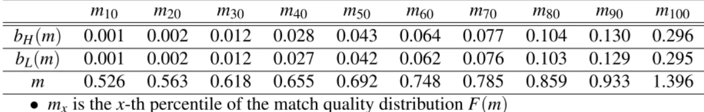
The pre-specified parameters are summarised in Tables3and4. The model is monthly, and I assign the discount factorβ to be 0.9967, implying an annual
inter-est rate of 4% which is the US average. Following Fujita and Ramey (2012), the vacancy creation costκ is set to be 0.0392.19 I assign µ, the worker’s bargaining
power, to be 0.5 following den Haan, Ramey and Watson (2000).
φH andφL are respectively the UI exhaustion rates during normal periods and recessions. I setφH to be 1/6 which implies the standard maximum UI duration of 26 weeks given the monthly frequency. As for the UI extensions during reces-sions, I sort them into four main UI duration groups: (1) 39 weeks for January 1948 - December 1971, (2) 52 weeks for January 1972 - December 1974 and July 1982 - September 1991, (3) 68 weeks for January 1975 - June 1982 and October 1991 - July 2008, and (4) 90 weeks for August 2008 - June 2014. These four du-rations are obtained by averaging the observed maximum UI dudu-rations over the respective periods when UI was extended. The valueφL changes and implies the maximum UI durations according to these UI duration regimes.20 I set ¯u to be 6.5% which historically has been used as a criterion in most UI extensions, albeit towards the upper end.
To determine the utility flow of type-iunemployed workers, hand, if insured,
bi(m), I use the results in Gruber (1997). In particular, the drop in consumption for newly unemployed workers is 10% when receiving UI and 24% when not
19Using survey evidence on vacancy durations and hours spent on vacancy posting, Fujita and Ramey (2012) find the vacancy cost to be 17% of a 40-hour-work week. Normalising the mean productivity to unity, this gives the value of 0.17 per week or 0.0392 per month. The actual mean productivity may be higher than (but not greatly different from) unity due to truncation from below of the match-specific quality.
20Note that these are the maximum UI durations used only when the unemployment rate is above the threshold ¯u. For example, in the simulation, the UI extension in the Great Recession is not triggered until April 2009.
receiving UI given the replacement rate of 50%.21 To find the impliedhandbi(m) given a set of parameters, I first guess the mean wages for the (type-i) employed with different match qualities{w0(m),wi0(m);∀m}and sethsuch that the average ratio ofhtow0(m)is 0.76 (where I use the steady state distribution of unemployed workers over match qualities to compute the weighted average).bi(m)is set such that the ratio ofh+bi(m)tow0i(m)is 0.9 for each match quality m. I then solve and simulate the model to check if the guess is close to its simulated counterpart. If it is not, I replace the guessed wages with the simulated ones and repeat until they are close enough.22
The slope of the unemployed’s search cost functionauis normalised such that the search effort of the uninsured unemployedsUU is unity when the economy is in the steady state, similar to Nagyp´al (2005). The power parameters in the search cost functions for both employed and unemployed workers (de anddu) are set to unity in line with Christensen, Lentz, and Mortensen (2005) and Yashiv (2000) implying a quadratic search cost function. As these parameters are important for the elasticity of unemployment duration with respect to the maximum UI dura-tion, I discuss in the next section how the results are comparable to the existing literature.
4.2
Calibrated Parameters
I use the simulated method of moments to assign values to the remaining twelve parameters {l,δ,λ,ψ,ξ,ae,m,β1,β2,ρz,σz,ηL} by matching main statistics in the US labour market and the labour productivity process during 1948-2007.23 The targeted moments are reported in Table2along with their empirical
counter-21Aguiar and Hurst (2005) report the drop in food consumption of workers upon becoming unemployed to be 5% and the drop in food expenditure to be 19%. However, in their study, unem-ployed workers are not distinguished by their UI status which makes it impossible to separately identifyhandbi(m)’s under the present calibration strategy.
22It is useful to note that there is a benefit cap in the US which varies from state to state. The average maximum UI benefit is around USD 441 per week. Given a 50-percent replacement rate, this implies that anyone whose income is above the 58th percentile will face a cap on their UI benefits in the US. Since the benefit levels are calibrated to match the consumption drops for newly unemployed workers, these benefits levels are in fact always smaller than half of the labour income at the 58th percentile in my model. Specifically, the maximum UI benefit payment in the model is 0.3 whereas the 58th percentile of the labour income is 0.73 implying a benefit cap at 0.36 with a 50-percent replacement rate.
23The transition rates are author’s own calculations based on the CPS data. For output, I use the quarterly real GDP series provided by the Bureau of Economic Analysis (BEA), and I use the BLS quarterly series for non-farm output per job to represent the labour productivity.
parts. Table6 shows other related moments not targeted in the calibration. The values of calibrated parameters are in Table5.
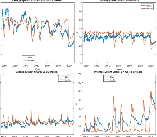
For targeted moments, the baseline model matches the twelve targeted mo-ments quite well overall. However, the insured unemployment rate is slightly higher, and the job finding rate is more volatile than in the data. For non-targeted moments, the model matches the dynamics of unemployment grouped in four du-ration bins quite well in terms of the first and second moments. However, the model could further improve on the volatility of vacancies and the correlation between unemployment and vacancies.24
5
Results
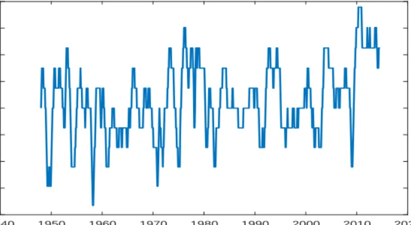
The results in this section are based on the aggregate productivity series that matches the deviations of output from its HP trend as depicted in Figure4.25
5.1
Performance
UI Extensions Figure5 shows that the model is successful in generating
real-istic UI extensions in terms of both when they are triggered and how long each extension lasts. This is due to how well the model replicates the US unemploy-ment series (of which UI extensions are a function) as shown in Figure6. The model does exceptionally well in capturing the dynamics of unemployment dur-ing the Great Recession. The series noticeably overshoots in the early 2000s. I address this issue in the last part of this subsection by correcting for the state-level implementation of UI extensions.
Long-term Unemployment Figure7 shows that the model can account for a
large fraction of the observed rise in long-term unemployment in the Great Reces-sion, but it tends to overshoot and does not produce enough persistence in certain recessions. The main reason for this is due to the sudden change in the opti-mal job search behaviour of insured unemployed workers when a UI extension is terminated, a mechanism that I will discuss in the next subsection.
24The main reason why vacancies are not as volatile as they are in the data is due to the endoge-nous separation margin. In recessions, unemployment increases at a faster rate from endogeendoge-nous match separations which makes vacancy posting less costly, and this counteracts with the effect of negative aggregate shocks.
25We can see that the drop in aggregate productivity during the Great Recession is neither of larger magnitude nor does it exhibit more persistence than in previous recessions.
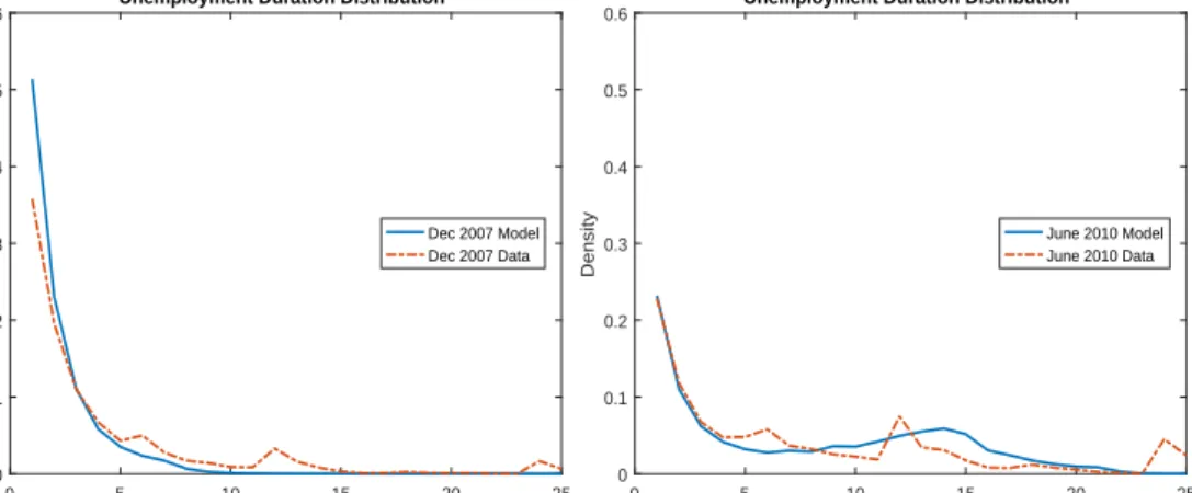
Distribution of Unemployment Duration Figure8shows that the model pro-duces a substantial rise in the average unemployment duration in the Great Re-cession, but, similar to long-term unemployment, it generates little persistence once compared to the data. It does very well in producing a realistic shift in the distribution of unemployment duration towards longer duration bins. In Figure9, I plot the distributions in December 2007 and June 2010, where UI was only ex-tended in the latter case.26 With respect to the entire 1948-2014 period, I show in Figure10the shares of unemployment by four duration bins (less than 1 month, 2-3 months, 4-6 months, and longer than 6 months). These figures suggest that the model is suitable for studying the dynamics of the entire distribution of un-employment duration and not just the long-term unun-employment dynamics.
Job Findings In the left panel of Figure11, I compare the model’s job finding
rate with the empirical series. Despite a clear negative trend that the model does not feature, it produces a fall in the job finding rate during the Great Recession similar in magnitude to that in the data. When I condition on the UI status of workers as displayed in the right panel of same figure, we can see that (1) the job finding rate of the insured unemployed workers is lower and falls more dramat-ically than that of the uninsured during the Great Recession. Both features are consistent with findings from the empirical section.
State-level Implementation of UI Extensions In the US, implementations of
UI extensions are at the state level. Therefore, it is possible that the maximum potential UI duration announced at the federal level does not coincide with the average maximum potential UI duration implemented across states, especially when only few states implement UI extensions. This is exactly the case in the early 2000 recession where only 5 states implemented UI extensions making the average maximum potential UI duration to be 30 weeks shorter than the federally announced maximum duration. This stark difference affects the model’s results significantly. Figure12 shows that, for the 2000 recession, total unemployment no longer overshoots (if anything, slightly undershoots) when the average UI du-ration is used in the simulation. As a result, UI extension is not triggered, and thus long-term unemployment is only mildly affected.
That said, the results for the Great Recession are robust to using the cross-state average of maximum UI duration since 49 cross-states actually implemented the
26I choose June 2010 because it is when the model’s long-term unemployment rate reaches its peak. Additionally, the model generates a hump in the distribution in 2010 similar to the empirical distribution owing to the endogenous separation margin.
extensions, and therefore the federally announced maximum UI duration is just 5 weeks longer than the average across states. Unfortunately, the state-level UI implementation data can be obtained from only 1999. However, as the focus of the paper is on the Great Recession, all the results during this episode are computed based on the actual implementation of UI extensions across states.27
5.2
Mechanisms
Job Search Behaviour The optimal job search behaviour of workers respond
to UI extensions in the following ways: (1) only the search intensity of insured unemployed workers varies with the maximum UI duration, and (2) the higher the benefit level the lower the search effort is exerted, and such behaviour is more pronounced when the extended UI duration is longer.
Figure13’s top left panel shows that the conditional job finding rate of the in-sured unemployed workers drops when UI is extended (implied byu≥u¯=6.5%) whilst the rates for the employed and uninsured unemployed are largely constant. Figure 13’s top right panel shows that, amongst the insured unemployed, job search effort decreases in the amount of benefit. In terms of worker heterogene-ity, higher productivity workers exert slightly more search effort as their value during employment is relatively higher than the lower productivity type. The job finding rates between the two productivity types during 1948-2014 are quite sim-ilar. However, when considering different UI statuses, the job finding rate of the insured unemployed is smaller and exhibits higher volatility. This suggests that once we condition on the UI status, workers’ productivity types contribute little to the rise of long-term unemployment and unemployment duration. Job findings are driven not only by the job search behaviour but also by the decision between a worker and a firm to form a match once they meet. Such decisions along with match separation decisions are also affected by the endogenous UI extensions as I discuss next.
Match Formation/Separation We know that the worker’s surplus from
be-ing employed and the value of a producbe-ing firm (W Sij(m;ω) and Jij(m;ω);j∈
{e(m˜),U I(m˜),UU}) are simply a constant fraction of a total match surplus (µSij(m;ω)
and (1−µ)Sij(m;ω) respectively). Therefore, both workers and firms always
agree when a match should be formed (whenSij(m;ω)>0) and when it should be
27More availability of the state-level UI implementation data would be useful in potentially explaining the overshooting of the long-term unemployment series.
separated (whenSij(m;ω)<0). A match surplus when a worker is currently
em-ployed,Sei(m˜)(m;ω), determines endogenous match separations whereas a match
surplus when a worker is currently unemployed, eitherSU Ii (m˜)(m;ω)orSUUi (m;ω),
determines how many matches will be formed, given that unemployed workers and firms have met.
Figure13’s bottom left panel shows that total match surpluses for employed and insured unemployed workers,Sei(m˜)(m;ω)andSU Ii (m˜)(m;ω), decrease in
un-employment, and they decrease at a faster rate when UI is extended (u≥u¯).28 The longer the extended duration, the more drastic is the drop in the match sur-plus. Further,SU Ii (m˜)(m;ω)decreases in ˜m in Figure13’s bottom right panel. A
higher ˜mimplies a higher outside option of the insured unemployed, h+bi(m˜), meaning that a match is less likely to be formed.29 A similar argument applies toSei(m˜)(m;ω)but, instead, on the job separation margin where h+bi(m˜)is the outside option of an employed worker if she quits and is eligible for UI.30
What Drives (Long-term) Unemployment? I study the contribution of 3 UI
channels (job search behaviour, match formation and job separation) on unem-ployment and its duration during the Great Recession by fixing/shutting down one channel at a time (assuming that a given channel does not respond to UI extensions).31 I find that long-term unemployment is largely unaffected by the response of match formation and dissolution but it falls drastically (over 3pp) when the job search channel is shut down as shown in Figure14. Despite a small impact on long-term unemployment, the job separation margin is most important in driving total unemployment.32
28It can be seen that the match surplus for the uninsured unemployed workers is higher when the UI extension is longer. This is because it is actually better for the uninsured unemployed to regain employment and potentially qualify for UI benefits.
29minstead increasesSU I(m˜)
i (m;ω)because a higher match quality in the production raises the
firm’s profit and the worker’s wage and potential UI benefit after being employed withm. 30In the simulation, the success rate of worker-firm meetings is, despite procyclical, always very close to one. The reasons are (1) for insured workers, those likely to have an unproductive meeting have currently high UI benefits, and it is unlikely for them to meet a firm in the first place, and (2) for uninsured workers, the surplus from working is very high due to their lower outside option which means the meetings are likely to lead to viable matches.
31Note that the path of aggregate shocks (z) is as in the baseline model (Figure4). I shut down a channel by setting the unemployment rate used in the respective policy function to be at the pre-Great Recession level which is less than ¯uimplying that UI is not extended.
32I also study the contribution of vacancy creation on long-term unemployment. However, its effect is small because the volatility of vacancies in the model is rather low relative to the data.
5.3
Policy Experiment
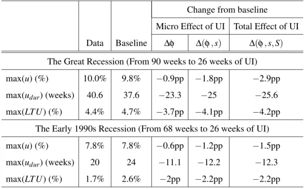
In this counterfactual exercise, I eliminate all UI extensions during the Great Recession (by increasing the UI exhaustion rate, φ(u), to φL implying a shorter maximum UI duration of 26 weeks) and quantify their effects on unemployment and its duration structure given the same path of aggregate productivity shocks (z) as in the baseline model (Figure4). I compute both the microeconomic and gen-eral equilibrium effects of UI. The former features only the higher UI exhaustion rate and the response of job search behaviour to the shorter UI duration, and it is comparable to results from the existing literature. The latter considers also the re-sponses of match separations and match formations to the shorter UI duration.33 Table7summarises the results from this experiment.
Long-term unemployment The removal of UI extension has a large impact
on long-term unemployment even when workers and firms do not react to this change. This is not surprising because, given the standard UI duration (of 26 weeks), all long-term unemployed workers are uninsured by definition, and unin-sured unemployed workers have a much higher job finding rate than do inunin-sured unemployed workers. As a result, by removing all UI extensions during the Great Recession, the peak of long-term unemployment falls drastically from 4.7 per-cent in the baseline model to 1 perper-cent when workers and firms do not react to the shorter maximum UI duration (as shown in Table7).34
Unemployment Total unemployment is less affected by the removal of UI
ex-tensions than long-term unemployment. The impact of increasing the UI exhaus-tion rate is a slight fall of less than 1pp in the unemployment rate (measured at its peak) as shown in Table 7. When the job search behaviour responds to the extension removal, the peak falls by 1.8pp. It is only in the general equilibrium context, where match separation decisions also react to the extension removal, that the peak of the unemployment rate falls by 2.9pp.
The microeconomic effect of UI on total unemployment is more subdued is because it concerns only a subgroup of unemployed workers (namely, those with
33It is clear from the previous decomposition exercise that the response of match formation to UI extensions is negligible.
34It is useful to note that the large microeconomic effect of UI on long-term unemployment relies on the higher job finding rate of uninsured unemployed workers when compared to the insured. By incorporating genuine duration dependence in the job finding rate, the UI effect could become smaller since unemployed workers who recently exhausted UI cannot increase their job finding rate as much as in the baseline model. Therefore, the insured unemployment state is less desirable and there will be fewer insured unemployed workers during UI extensions.
UI), whilst for the general equilibrium effect, the match separation margin ap-plies to all employed workers and determines the inflow of (insured) unemployed workers. This same argument also explains why the micro effect of UI on long-term unemployment is large.
This result is consistent with the existing literature on the effects of UI exten-sions on unemployment in the Great Recession. Most of the studies focus on the micro effect where the worker-firm relationships are not taken into account and find that the unemployment rate would have been 0.1-1.8pp lower had there been no UI extensions. This is in line with the micro effect of UI extensions previ-ously discussed. The larger general equilibrium effect of UI extensions in this model is similar to findings in Hagedorn et al. (2019), but they focus the im-pact on vacancy creation whilst mine comes from job separations.35 Lastly, the unemployment rate is much less persistent when there is no UI extensions, i.e. there would be no jobless recoveries. This result is consistent with the findings in Mitman and Rabinovich (2014).
Non-linearity of UI effects In Table 7, I also report the effects of removing
UI extensions during the early 1990s recession (equivalent of cutting 42 weeks of UI duration). There is a non-linearity of the UI effects on all variables con-sidered. For example, a one-week reduction of UI duration reduces an average unemployment duration by 0.3 weeks during the 1990s recession36 but for the Great Recession this number is 0.4 weeks. This is mainly due to the different paths of shocks that hit the economy. As can be seen in Figure4, the Great Re-cession features a larger but less persistent negative shock comparing to the early 1990s recession. This suggests that the unemployment cost of UI extension is less pronounced when a recession is more persistent (e.g. the early 1990s) since it is more difficult for workers to find a job regardless of the maximum UI duration.
5.4
Reachback Provision Programme
From May 2007, the Emergency Unemployment Compensation law has in-cluded the “Reachback Provision” providing UI eligibility to unemployed work-ers who have already exhausted their benefits prior to the UI extensions. This
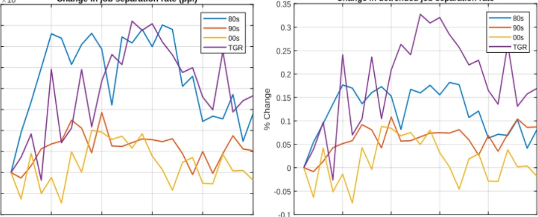
35Figure15shows that indeed the empirical job separation rate was particularly high during the Great Recession when compared to other recessions.
36If we only consider the micro effect of UI extensions, this number is around 0.26 for the 1990s recession which is still higher than the existing empirical findings of around 0.1-0.2. See, for example, Katz and Meyer (1990), Moffitt (1985), and Moffitt and Nicholson (1982).
programme can potentially affect long-term unemployment since it is targeted directly at this group of workers. As the programme is already incorporated in the baseline case, I can measure its effect by removing the programme and leav-ing everythleav-ing else the same. The results are summarised in Table8. I find that Reachback Provision does not have a significant impact on the aggregate labour market. The (long-term) unemployment rate is only 0.1pp smaller than in the baseline model. The small effect is explained by the fact that the subgroup of workers who are affected by the programme represents just 3.5% of the unem-ployment population. However, from the CPS data, the true effect of this pro-gramme could be non-trivial since unemployed workers who already exhausted UI represented a substantial 44% of the long-term unemployed in January 2008. The model produces a much smaller number for this group of workers because once the insured unemployed exhaust their benefits, they adopt the job search be-haviour of the uninsured which implies a much higher unemployment exit rate than the insured.
5.5
Rational Expectations
As a high unemployment rate triggers UI extensions, agents can form expec-tations about future unemployment to gauge the probability that a UI extension occurs or terminates. To quantify the importance of rational expectations about the timing of UI extensions, I compare the baseline results to an alternative sce-nario where UI extensions (and how long they last) are completely unexpected to the agents. This is the ‘adaptive expectations’ in Mitman and Rabinovich (2014) where agents assume the maximum UI duration to remain the same until they observe otherwise. This new UI duration policy is just a constant instead of a function of unemployment, i.e. φ instead of φ(u). When UI extensions are
as-sumed to last forever, the UI effects are expected to be more drastic because (1) the insured unemployed will lower search effort, (2) matches are less likely to be formed, and (3) matches are more likely to separate. I find that disregarding rational expectations about the timing of UI extensions leads to a significant over-estimation of both total and long-term unemployment by over 2pp at the peak of the Great Recession and an overestimation of average unemployment duration by almost 4 weeks as shown in Table8. Therefore, it is vital that rational expecta-tions are taken into account when studying the effects of UI extensions in general equilibrium.
5.6
On-the-job Search
In this exercise, I show how on-the-job search contributes to unemployment and its duration distribution during the Great Recession. On the one hand, on-the-job search allows employed workers to improve their match qualities and the associated UI benefits if they become insured unemployed. Since the job search effort and job finding rates are decreasing in the benefit level, this would increase unemployment and its duration. On the other hand, on-the-job search increases the value of being employed. Therefore, more unemployed workers would be in-duced to take up job offers even when the first match quality draws are not great (since they can search on the job and leave their current matches with not so great match qualities) and spend less time in unemployment. The last column of Table
8shows the main results when on-the-job search is not allowed. I find that, during the Great Recession when UI is extended, on-the-job search contributes to a small but significant increase in (long-term) unemployment of up to (0.4) 0.5pp from the baseline model as well as a 1-week increase in the average unemployment du-ration. On-the-job search, however, has a negligible impact outside recessionary periods.
5.7
Hazard Rate of Exiting Unemployment
Due to the heterogeneity in job finding rates amongst unemployed workers, the model generates the negative duration dependence in the unemployment exit rate that comes purely from the changing composition in the stocks of unem-ployment.37 At longer unemployment durations, the stocks of unemployment are more represented by those with lower exit rates (the insured unemployed with higher UI benefits in this case). Moreover, the strength of the duration depen-dence is positively correlated with the state of the economy as pointed out in Wiczer (2015). Figure16 shows the hazard rates of exiting unemployment for December 2007 (maximum 26 weeks of UI) and June 2010 (maximum 90 weeks of UI). The negative duration dependence is more severe with and persists as long as the UI extensions themselves. Empirical results based on Kroft et al. (2016) and Wiczer (2015) suggest that the hazard rate is stable after 6 months of being unemployed. In the model, however, since uninsured unemployed workers exit
37The duration-dependent unemployment exit rate is a featured result in several studies in-cluding Clark and Summers (1979), Machin and Manning (1999), and Elsby, Hobijn, S¸ahin and Valletta (2011).
unemployment at a faster rate than do the insured, the hazard rate rises upon the exhaustion of UI benefits.38
To study the role of unobserved heterogeneity, I estimated the same non-linear state space model in Ahn and Hamilton (2019). They find that the unobserved heterogeneity of workers (in terms of unemployment exit rate) contribute to the rise in unemployment duration during the Great Recession. I can relate their interpretation of unobserved heterogeneity to the UI status in my model as the insured unemployed have a lower unemployment exit rate than the uninsured. I find little differences in the unemployment exit rate based on the heterogeneous worker productivity. I describe in full the state space model, the estimation and the results in Appendix E and F.
6
Conclusion
This paper quantifies the impact of endogenous UI extensions on the dynamics of unemployment and its duration structure which have an important implication on the recovery of the aggregate labour market. I develop a general equilibrium search and matching model where the maximum UI duration depends on the un-employment rate, and the UI benefits depend on the match quality during em-ployment. Workers are heterogeneous and their job search effort depend on their characteristics as well as the maximum UI duration.
I find that the generous UI extensions during the Great Recession contribute to 10-30% of the rise of unemployment. Both the microeconomic and general equilibrium effects of UI are important and the former is consistent with exist-ing empirical estimates. The UI effect on long-term unemployment is, however, much larger as it contributes up to 90% of its rise where the microeconomic effect of UI is most responsible. That said, the UI effect is non-linear as its magnitude is smaller in the early 1990s recession. I also show that disregarding rational ex-pectations about the timings of UI extensions implies a significant overestimation of the UI effects on unemployment and its duration.
38The heterogeneity in worker productivity could potentially explain the negative duration de-pendence after the UI exhaustion since type-Hworkers exit unemployment at a faster rate. How-ever, despite this heterogeneity, the exit rates of both types (HandL) when uninsured are similar and much higher than when insured which leaves the average exit rate after UI exhaustion rather stable. In order to fit the empirical results better, other heterogeneity amongst uninsured unem-ployed workers could be introduced such as different values of home production, or even a larger degree of heterogeneity in productivity.
References
[1] Aaronson, Daniel, Bhashkar Mazumder, and Shani Schechter, 2010. “What is behind the rise in long-term unemployment?”, Economic Perspectives, QII, pp. 28-51.
[2] Abraham, Katharine G., John C. Haltiwanger, L. Kristin Sandusky, and James R. Spletzer, 2016. “The Consequences of Long Term Unemploy-ment: Evidence from Matched Employer-Employee Data”,IZA Discussion Papers, no. 10223.
[3] Aguiar, Mark and Erik Hurst, 2005. “Consumption versus Expenditure”,
Journal of Political Economy, 113, pp. 919-948.
[4] Ahn, Hie Joo, 2016. “The Role of Observed and
Unob-served Heterogeneity in the Duration of Unemployment Spells”,
https://sites.google.com/site/hiejooahn/research.
[5] Ahn, Hie Joo and James D. Hamilton, 2019. “Heterogeneity and Unem-ployment Dynamics”, Journal of Business & Economic Statistics, DOI: 10.1080/07350015.2018.1530116.
[6] Barnichon, Regis and Andrew Figura, 2014. “The Effects of Unemployment Benefits on Unemployment and Labor Force Participation: Evidence from 35 Years of Benefits Extensions”,Finance and Economics Discussion Series 2014, no. 65, Board of Governors of the Federal Reserve System (US). [7] Card, David, Phillip B. Levine, 2000. “Extended benefits and the duration of
UI spells: evidence from the new Jersey extended benefit program”,Journal
of Public Economics, 78 (1–2), pp. 107-138.
[8] Carrillo-Tudela, Carlos and Ludo Visschers, 2014.
“Unemploy-ment and Endogenous Reallocation over the Business Cycle”,
https://sites.google.com/site/ludosresearch/.
[9] Clark, Kim B. and Lawrence H. Summers, 1979. “Labor Market Dynamics and Unemployment: A Reconsideration”, Brookings Papers on Economic Activity, 10, 13-72.
[10] Christensen, Bent J., Rasmus Lentz, Dale T. Mortensen, George R. Neu-mann, and Axel Werwatz, 2005. “On-the-job search and the wage distribu-tion”,Journal of Labor Economics, 23(1), pp. 31–58.
[11] den Haan, Wouter J., Garey Ramey and Joel Watson, 2000. “Job Destruction and Propagation of Shocks”, American Economic Review, 90(3), pp. 482-498.
[12] Elsby, Michael W. L., Bart Hobijn, Ays¸eg¨ul S¸ahin and Robert G. Valletta, 2011. “The Labor Market in the Great Recession-An Update to September 2011”,Brookings Papers on Economic Activity, 2011(2), pp. 353-384. [13] Faig, Miguel, Min Zhang and Shiny Zhang, 2016. “Effects of Extended
Unemployment Benefits on Labor Dynamics”, Macroeconomic Dynamics, 20(05), pp. 1174-1195.
Unemploy-ment Benefits Lengthen UnemployUnemploy-ment Spells? Evidence from Recent Cy-cles in the U.S. Labor Market”,NBER Working Papers, no. 19048.
[15] Fredriksson, Peter and Bertil Holmlund, 2001. “Optimal Unemployment In-surance in Search Equilibrium”, Journal of Labor Economics, 19(2), pp. 370-399.
[16] Fujita, Shigeru and Garey Ramey, 2012. “Exogenous versus Endogenous Separation”, American Economic Journal: Macroeconomics, 4(4), pp. 68-93.
[17] Fujita, Shigeru, 2010. “Effects of the UI Benefit Extensions: Evidence from the CPS”, Federal Reserve Bank of Philadelphia Working Paper, No. 10-35/R.
[18] Fujita, Shigeru and Giuseppe Moscarini, 2015. “Recall and unemployment”,
Federal Reserve Bank of Philadelphia Working Paper, No. 14-3.
[19] Gruber, Jonathan, 1997. “The Consumption Smoothing Benefits of Unem-ployment Insurance”,American Economic Review, 87(1), pp. 192-205.
[20] Hagedorn, Marcus, Fatih Karahan, Iourii Manovskii, and
Kurt Mitman, 2019, “Unemployment Benefits and
Unemploy-ment in the Great Recession: The Role of Macro Effects”,
https://www.sas.upenn.edu/∼manovski/research.html.
[21] Hornstein, Andreas, 2012. “Accounting for Unemployment: The Long and Short of It”,Federal Reserve Bank of Richmond Working Paper, no. 12-07. [22] Katz, Lawrence F. and Bruce D. Meyer, 1990. “The impact of the
poten-tial duration of unemployment benefits on the duration of unemployment”,
Journal of Public Economics, 41(1), pp. 45-72.
[23] Kroft, Kory, Fabian Lange, Matthew J. Notowidigdo and Lawrence F. Katz, 2016. “Long-Term Unemployment and the Great Recession: The Role of Composition, Duration Dependence, and Non-Participation”,Journal of
La-bor Economics, 34, no. S1 (Part 2, January 2016): S7-S54.
[24] Krause, Michael and Thomas A. Lubik, 2010. “On-the-job search and the cyclical dynamics of the labor market”,Federal Reserve Bank of Richmond
Working Paper, no. 10-12.
[25] Krueger, Alan B. and Andreas Mueller, 2010. “Job search and unemploy-ment insurance: new evidence from time use data”, Journal of Public
Eco-nomics, 94(3–4), pp. 298-307.
[26] Krueger, Alan B. and Andreas Mueller, 2011. “Job search, emotional well-being and job finding in a period of mass unemployment: evidence from high frequency longitudinal data”,Brookings Papers on Economic Activity, 42, pp. 1–81.
[27] Krusell, Per and Anthony A. Smith Jr., 1998. “Income and wealth hetero-geneity in the macroeconomy”,Journal of Political Economy, 106, pp. 867-896.
[28] Machin, Steve and Alan Manning, 1999. “The causes and consequences of longterm unemployment in Europe”. In O. Ashenfelter and D. Card (Ed.),
Handbook of Labor Economics. Handbooks in economics, 3C(5). Elsevier B.V, Amsterdam, Holland, pp. 3085-3139.
[29] Mazumder, Bhashkar, 2011. “How did unemployment insurance extensions affect the unemployment rate in 2008–10?”,Chicago Fed Letter, no. 285. [30] Meyer, Bruce D., 1990. “Unemployment insurance and unemployment
spells”,Econometrica, 58(4), pp. 757-782.
[31] Mitman, Kurt and Stanislav Rabinovich, 2014. “Do
Unemploy-ment Benefits Explain the Emergence of Jobless Recoveries?”,
http://www.kurtmitman.com.
[32] Moffitt, Robert, 1985. “Unemployment insurance and the distribution of un-employment spells”.Journal of Econometrics, 28(1), pp. 85-101.
[33] Moffitt, Robert, Nicholson, Walter, 1982. “The effect of unemployment in-surance on unemployment: the case of federal supplemental benefits”, Re-view of Economics and Statistics, 64(1), pp. 1-11.
[34] Mortensen, Dale T. and Christopher A. Pissarides, 1994. “Job Creation and Job Destruction in the Theory of Unemployment”, Review of Economic Studies, 61(3), pp. 397-415.
[35] Nakajima, Makoto, 2012. “A quantitative analysis of unemployment benefit extensions”,Journal of Monetary Economics, 59(7), pp. 686-702.
[36] Nagyp´al, Eva,´ 2005. “On the extent of job-to-job transitions”,
http://faculty.wcas.northwestern.edu/∼een461/research.html.
[37] Ravn, Morten O. and Vincent Sterk, 2017. “Job Uncertainty and Deep Re-cessions”,Journal of Monetary Economics, 57 (2), pp. 217-225.
[38] Rothstein, Jesse, 2011. “Unemployment Insurance and Job Search in the Great Recession”,NBER Working Papers, no. 17534.
[39] Rouwenhorst, K. Geert, 1995. “Asset pricing implications of equilibrium business cycle models”. In: Cooley, T. F. (Ed.),Frontiers of Business Cycle
Research. Princeton University Press, Princeton, NJ, pp. 294-330
[40] Rujiwattanapong, W. Similan, 2017. “Unemployment
Insur-ance and Labour Productivity over the Business Cycle”,
https://sites.google.com/site/wsrujiwattanapong/home/research.
[41] Shimer, Robert, 2006. “On-the-job search and strategic bargaining”,
Euro-pean Economic Review, 50(4), pp. 811-830.
<