Wavelet Analysis of Nonstationary Circadian Time Series

Wavelet Analysis of Nonstationary Circadian

Time Series

Jessica Kate Hargreaves

P

D

U

NIVERSITY OF

Y

ORK

M

ATHEMATICS

Abstract

Rhythmic data are ubiquitous in the life sciences, with biologists needing reliable sta-tistical tools for the analysis of such data. When these signals display rhythmic yet non-stationary behaviour, common in many biological systems, the established methodologies are often misleading.

Chapter 2 develops and tests a new method for clustering nonstationary rhythmic bio-logical data. The method combines locally stationary wavelet time series modelling with functional principal components analysis and thus extracts time—scale patterns useful for identifying common characteristics. We demonstrate the advantages of our methodology over alternative approaches by means of a simulation study and for real circadian data ap-plications.

Motivated by three complementary applications in circadian biology, Chapter 3 devel-ops new reliable statistical tests to identify whether a particular experimental treatment has caused a significant change in a rhythmic signal that displays nonstationary charac-teristics. As circadian behaviour is best understood in the spectral domain, we develop novel hypothesis testing procedures in the (wavelet) spectral domain, which facilitate the identification of three specific types of spectral difference. We demonstrate the advantages of our methodology over alternative approaches by means of a comprehensive simulation study and for real data applications, involving both plant and animal signals.

Chapter 4 investigates the effect of industrial and agricultural pollutants on the plant circadian clock. We examine the impact of exposure to a comprehensive range of environ-mentally relevant pollutants by utilising the methodologies developed in Chapters 2 and 3. Our findings indicate that many of the tested chemicals have an effect on the plant circa-dian clock, most of which would have remained undetected by classical methods overlook-ing nonstationarity. The results of Chapter 4 demonstrate the additional insight gained by using the appropriate methodologies, as developed in Chapters 2 and 3, and also have im-portant implications for understanding environmental ramifications associated with soil pollution.

Contents

1.2.2 The Discrete Wavelet Transform (DWT) . . . 31

1.2.3 Matrix Representation of the Discrete Wavelet Transform . . . 35

1.2.4 The Nondecimated Wavelet Transform . . . 36

1.3 Stationary Time Series Analysis . . . 40

1.3.1 Fourier Analysis of Stationary Time Series . . . 41

1.3.2 Stationary Time Series Analysis of Circadian Data . . . 42

1.3.3 Wavelet Analysis of Stationary Time Series . . . 47

1.4 Nonstationary Time Series Analysis . . . 47

1.4.1 Locally Stationary Time Series . . . 48

1.4.2 Locally Stationary Wavelet Model . . . 50

1.4.3 Nonstationary Time Series Analysis of Circadian Data . . . 52

2 Clustering Nonstationary Circadian Rhythms Using Locally Stationary Wavelet Rep-resentations 55 2.1 Introduction . . . 55

2.2 Motivation . . . 56

2.2.1 Experimental Details . . . 57

2.2.2 BRASS Analysis . . . 57

2.2.3 Nonstationarity in Circadian Rhythms . . . 58

2.2.4 Individual-level Variability in Circadian Rhythms . . . 58

2.3 Proposed Clustering Method . . . 59

2.3.2 Overview of Current Clustering/Classification Techniques that Account for

Nonstationarity . . . 60

2.3.3 Proposed Functional Principal Components Analysis for the Wavelet Spec-tral Content . . . 62

2.3.4 Proposed Clustering Method . . . 63

2.4 Simulation Study . . . 67

2.4.1 Simulated Data . . . 67

2.5 Results . . . 70

2.6 Real Data Analysis . . . 72

2.6.1 Previously Published Circadian Data . . . 72

2.6.2 Novel Circadian Plant Data . . . 77

2.7 Conclusions and Further Work . . . 81

2.8 Appendix: Supplementary Figures . . . 83

2.9 Appendix: Experimental Details: Novel Circadian Plant Data . . . 86

2.10 Appendix: Results of Simulation Study Cases 1 and 4 . . . 87

2.11 Appendix: Experimental Details: Previously Published Circadian Data . . . 88

3 Wavelet Spectral Testing: Application to Nonstationary Circadian Rhythms 89 3.1 Introduction and Motivation . . . 89

3.1.1 Motivating Datasets . . . 89

3.1.2 Aims and Structure of this Chapter . . . 92

3.2 Overview: Nonstationary Processes and Hypothesis Testing in the Spectral Domain 92 3.2.1 Modelling Nonstationary Processes . . . 92

3.2.2 Existing Spectral Domain Hypothesis Testing . . . 94

3.3 Proposed Spectral Domain Hypothesis Tests . . . 96

3.3.1 Lead Dataset: Hypothesis Testing for Spectral Equality (‘WST’ and ‘FT’) . . 96

3.3.2 Ultradian Dataset: Hypothesis Testing for Spectral Equality Across Scales (‘HFT’) . . . 99

3.3.3 Nematode Dataset: Hypothesis Testing for ‘Same Shape’ Spectra (‘HT’) . . 100

3.3.4 Summary . . . 101 3.4 Simulation Studies . . . 102 3.4.1 Power Comparisons . . . 103 3.4.2 Size Comparisons . . . 105 3.4.3 Sensitivity Analysis . . . 107 3.4.4 Summary of Findings . . . 108

3.5 Real Data Analysis: Back to the Motivating Circadian Datasets . . . 108

3.5.1 Lead Dataset . . . 109

3.5.2 Ultradian Dataset . . . 109

3.5.3 Nematode Dataset . . . 110

3.6 Conclusions and Further Work . . . 112

3.7 Appendix: Experimental Details . . . 114

3.7.1 Experimental Overview: Lead and Ultradian Datasets . . . 114

3.7.2 Lead Nitrate Dataset . . . 114

3.7.3 Ultradian Dataset . . . 114

3.8 Appendix: Real Data Analysis: Supplementary Material . . . 116

3.9 Appendix: Tenability of the Normality Assumption . . . 117

3.10 Appendix: Haar-Fisz Transform . . . 118

3.11 Appendix: Detailed Description of Simulation Studies . . . 119

3.11.1 Detailed Description of Adaptive Neyman Test . . . 119

3.11.2 Basic Structure of Hypothesis Tests and Model Details . . . 121

3.11.3 Supplementary Tables . . . 127

3.12 Appendix: Summary Table . . . 133

4 Investigating the Effect of Soil Pollution on the Plant Circadian Clock 134 4.1 Introduction and Motivation . . . 134

4.2 Experimental Details . . . 135

4.3 Traditional Fourier Analysis . . . 136

4.3.1 Discussion of Findings . . . 136

4.3.2 Testing for Stationarity . . . 139

4.4 Wavelet Spectral Testing Using the Methodology Developed in Chapter 3 . . . 141

4.4.1 Discussion of Findings . . . 141

4.4.2 Conclusions . . . 147

4.5 Extension to Other Chemicals . . . 148

4.5.1 Discussion of Findings . . . 148

4.5.2 Conclusions . . . 154

4.6 Cluster Analysis Using the Methodology Developed in Chapter 2 . . . 154

4.6.1 Clustering DEFRA Chemicals . . . 155

4.6.2 Discussion of Findings . . . 155

4.6.3 Example: Clustering Within Individual Microtiter Plates . . . 155

4.6.4 Discussion of Findings . . . 156

4.7 Conclusions and Further Work . . . 159

4.8 Appendix: Supplementary Tables . . . 161

4.9 Appendix: Additional Clustering Example . . . 164

4.9.1 Discussion of Findings . . . 164

5 Conclusions and Further Work 167

List of Tables

1 Summary of the output of the analysis of the circadian dataset in BRASS. The ‘number of plants excluded by BRASS’ is the number of time series for which BRASS was not able to return a period estimate. ‘RAE’ (Relative Amplitude Er-ror) is a value between 0 and 1 and gives information about the goodness of fit of the model (a value of 0 indicates a perfect fit). Results with an RAE over 0.4 are discarded. Recall: there are 24 plants in each of the groups. . . 58 2 Results for the Priestley-Subba Rao test of stationarity, implemented in thefractal

package in R and available from the CRAN package repository. Number of non-stationary plants indicates the number of time series (in each group) with enough evidence to reject the null hypothesis of stationarity at the 1% significance level. Recall: there are 24 plants in each of the groups. . . 59 3 Case 4. The abruptly changing parameters of two nonstationary autoregressive

processes. . . 70 4 Comparison of the proposed LSW-PCA clustering method with the methods

pro-posed by Rouyer et al. (2008) and Antoniadis et al. (2013) for the simulation stud-ies. Percentages show correct clustering rates. . . 72 5 Results of clustering the copper dataset into two clusters using the proposed

LSW-PCA method. The modal cluster for each copper regime is highlighted in bold. . 74 6 Results of clustering the (normalised, truncated) cerium dataset into three groups

using the proposed LSW-PCA method. The modal cluster for each concentration is highlighted in bold. . . 77 7 Distance measure (Section 2.3.4.1) comparison for the proposed LSW-PCA method

for Cases 1 and 4. . . 87 8 Case 1: Comparison for selection of principal components for proposed

LSW-PCA clustering method. Percentages show correct clustering rates. . . 87 9 Case 4: Comparison for selection of principal components for proposed

LSW-PCA clustering method. Percentages show correct clustering rates. . . 87 10 Wavelet information comparison for the proposed LSW-PCA method for Cases 1

and 4. Percentages show correct clustering rates. . . 87 11 A summary of the hypothesis tests developed in this chapter. . . 102 12 Simulated power estimates (%) for models P1-P7 with nominal size of 5% with

N1=N2=25 realisations from each group. Highest empirical power estimates are highlighted in bold. . . 104 13 Performance Comparison: Simulated power estimates (%) for models P8-P12

with nominal size of 5% withN1=N2=25 realisations from each group and using the false discovery rate procedure (FDR). Note: Control group period is 24 hours in each model. . . 105 14 Simulated size estimates (%) for models M1-M4 with nominal size of 5% andN1=

N2=25 realisations from each group. Empirical size estimates over the nominal size of 5% are highlighted in bold. . . 107

15 The number of rejections (as a percentage in brackets) for each relevant pro-posed test and multiple-hypothesis testing procedure for the motivating example datasets. . . 109 16 A summary of the output of the analysis of the motivating example datasets in

BRASS: the mean period estimate for the control and test groups in hours (ob-tained using FFT-NLLS analysis (Plautz et al., 1997)), the difference between the period estimates and the corresponding p–value. . . 116 17 Results for the Priestley-Subba Rao test of stationarity, implemented in thefractal

package in R and available from the CRAN package repository. Number of non-stationary plants indicates the number of time series (in each motivating example dataset) with enough evidence to reject the null hypothesis of stationarity at the 5% significance level (as a percentage in brackets). . . 116 18 P6: AR Processes with Abruptly Changing Parameters. The abruptly changing

parameters of two nonstationary autoregressive processes. . . 124 19 P7: AR Processes With Slowly Changing Parameters. The slowly changing

pa-rameters of two nonstationary autoregressive processes. . . 125 20 Simulated power and size estimates (%) for the HFT for models P1-P7 and M1-M4

with nominal size of 5% andN1=N2=1 realisation from each group. . . 127 21 Simulated power estimates (%) for models P1-P7 with nominal size of 5%. N =

N1=N2is the number of realisations in each group. Highest empirical power estimates are highlighted in bold. . . 127 22 Simulated size and power estimates (%) for models P8-P12 and M5 with nominal

size of 5% and using the false discovery rate procedure (FDR).N=N1=N2is the number of realisations in each group. Note: Control group period is 24 hours in each model. . . 128 23 Simulated size estimates (%) for models M1-M4 with nominal size of 5%. N =

N1=N2 is the number of realisations in each group. Empirical size estimates over the nominal size of 5% are highlighted in bold. . . 128 24 M4: AR Process with Slowly Changing Parameters. Numbers of rejections in

empirical size estimates for theRaw Periodogram F-Test(FT), with Bonferroni Correction (Bon.) and false discovery rate (FDR) and with nominal size of 5%. “Modified Empirical Size Estimate” is calculated by examining only cases with more than one significant coefficient. . . 128 25 Potential Non-Gaussian Innovations: Simulated size and power estimates (%)

for models P1-P5 and M1, M2 with nominal size of 5% andN1=N2=25 realisa-tions from each group. Innovarealisa-tions are distributed as: standard normal (denoted N(0,1)) or t-distribution with 5 or 3 degrees of freedom (denotedt5, t3 respec-tively). For the FT, the modified size and power estimates are recorded (i.e. only consider cases when more than 5 rejections are reported– see Section 3.4.2). Em-pirical size estimates over the nominal size of 5% are highlighted in bold. . . 129

26 Potential Non-Gaussian Errors:Simulated size and power estimates (%) for mod-els P8-P12 and M5 with nominal size of 5% andN1=N2=25 realisations from each group. The noise term in equation (105) is distributed as: standard normal (denoted N(0,1)) or t-distribution with 5 or 3 degrees of freedom (denotedt5,t3 respectively). For the FT, the modified size and power estimates are recorded (i.e. only consider cases when more than 5 rejections are reported– see Section 3.4.2). Empirical size estimates over the nominal size of 5% are highlighted in bold. . . 130 27 Sensitivity to Generation and Estimation Wavelet Mismatch:Simulated size and

power estimates (%) for models P1-P5 and M1, M2 with nominal size of 5% and N1=N2=25 realisations from each group. In all settings, the Haar wavelet is used for spectral estimation, but the following wavelets are used to generate the true spectra: Haar wavelets, Daubechies’ least-asymmetric wavelets with 4 vanishing moments (V.M.) and Daubechies’ extremal phase wavelets with 10 vanishing mo-ments, respectively. . . 131 28 Sensitivity to the Change of Modelling Wavelet:Simulated power estimates (%)

for models P6-P12 with nominal size of 5% andN1=N2=25 realisations from each group. Different wavelets are used for the wavelet spectral estimation: Haar wavelets, Daubechies’ least-asymmetric wavelets with 4 vanishing moments (V.M.) and Daubechies’ extremal phase wavelets with 10 vanishing moments, respectively.132 29 A summary of the hypothesis tests developed in this chapter. . . 133 30 BRASS Results– DEFRA Chemicals. Summary of the output of the analysis of the

DEFRA chemicals in BRASS. “Treatment” represents the element under investi-gation within the chemical compound.∗indicates a significant change in period from the respective control group. † denotes an RAE value above the 0.4 thresh-old. “Number Analysed” is the number of time series for which BRASS was able to return a period estimate. There are 24 plants in each treatment group. ‡ Note that the Lead (Max) treatment group coincides with the ‘Lead dataset’ from Chapter 3. 137 31 Results for the Priestley-Subba Rao test of stationarity, implemented in thefractal

package in R and available from the CRAN package repository. Number of nonsta-tionary time series indicates the number of time series (in each treatment group) with enough evidence to reject the null hypothesis of stationarity at the 5% sig-nificance level (as a percentage in brackets). . . 141 32 FT (FDR) results– DEFRA Chemicals. The number of rejections (as a

percent-age in brackets) for the FT with FDR (at the 5% significance level) for the DEFRA Chemicals with † denoting 0% rejections. “Treatment” represents the element under investigation within the chemical compound. The estimated mean differ-ence in period (using FFT–NLLS) is also shown for referdiffer-ence with∗indicating a significant change in period from the respective control group. . . 142 33 Results of clustering plate 0953 into two clusters using the proposed LSW-PCA

method. The modal cluster for each treatment group is highlighted in bold. . . . 156 34 FT (FDR) results– DEFRA Chemicals (plate 0953). The number of rejections (as

a percentage in brackets) for the FT with FDR (at the 5% significance level) for the DEFRA Chemicals (plate 0953). . . 158

35 Extension chemicals Part 1(atomic numbers 3–27). The chemicals and concen-trations used in the salt stress experiment (Section 4.5), where “Treatment” rep-resents the element under investigation within the chemical compound (corre-sponding to the periodic table representation used in Figure 52) and “AN” repre-sents the associated atomic number. For each chemical, the number of rejections (as a percentage in brackets) for the FT with FDR (at the 5% significance level) and the estimated mean difference in period (using FFT–NLLS), with∗indicating a significant change in period from the respective control group. ‡ indicates time series and a barcode plot for the chemical are shown in Figures 53 or 54. . . 161 36 Extension chemicals Part 2(atomic numbers 37–83). The chemicals and

con-centrations used in the salt stress experiment (Section 4.5), where “Treatment” represents the element under investigation within the chemical compound (cor-responding to the periodic table representation used in Figure 52) and “AN” rep-resents the associated atomic number. For each chemical, the number of rejec-tions (as a percentage in brackets) for the FT with FDR (at the 5% significance level) and the estimated mean difference in period (using FFT–NLLS), with∗ in-dicating a significant change in period from the respective control group. ‡ indi-cates time series and a barcode plot for the chemical are shown in Figures 53 or 54. . . 162 37 Results of clustering the 12 DEFRA Chemicalsin Figures 47 and 48 and their

respective controls into 2 groups using the LSW-PCA method. There are 24 plants in each treatment group.∗indicates a treatment with 0 plants in cluster 2. . . 163 38 Results of clustering plate 0952 into three clusters using the proposed LSW-PCA

method. The modal cluster for each treatment group is highlighted in bold. . . . 164 39 FT (FDR) results– Comparing DEFRA Chemicals (plate 0952). The number of

rejections (as a percentage in brackets) for the FT with FDR (at the 5% significance level) for the DEFRA Chemicals (plate 0952). . . 166

List of Figures

1 Example 1.1.3. Dashed black line: Underlying cosine curve with a frequency of 1/(2∆t)=0.5 (i.e. the Nyquist frequency) and an amplitude of 2; Dashed blue line: Underlying cosine curve with a frequency of 1=2×1/(2∆t) (i.e. double the Nyquist frequency) and an amplitude of 2; Black circles: Observed value of underlying functions att=1, 2, . . . , 5. . . 25 2 Example 1.1.6. Top left: First underlying cosine curve with a frequency of 6/128

and an amplitude of 2; Top right: Second underlying cosine curve with a fre-quency of 10/128 and an amplitude of 4; Bottom left: The time series is a linear combination of two underlying cosine curves (see equation (3)); Bottom right: raw periodogram of the series with the frequencies 6/128 and 10/128 indicated by vertical red lines and horizontal green lines indicating values of 4 and 16 (which correspond to the amplitudes of the underlying cosine components squared– see equation (3)). . . 26 3 Example 1.1.7. Top left: First underlying cosine curve with a frequency of 6/128

and an amplitude of 2; Top right: Second underlying cosine curve with a fre-quency of 10/128 and an amplitude of 4; Bottom left: The time series is the con-catenation of the two cosine curves (see equation (4)); Bottom right: raw peri-odogram of the series with the frequencies 6/128 and 10/128 indicated by verti-cal red lines and horizontal green lines indicating values of 4 and 16 (which cor-respond to the amplitudes of the underlying cosine components squared– see equation (4)). . . 27 4 Panel (a): Haar mother wavelet. Panels (b), (c), (d): translations and dilations of

the Haar mother wavelet (using equation (10) for various combinations ofj=1, 2 andk=1, 2). . . 29 5 Successive approximations of the Doppler test function introduced by Donoho

and Johnstone (1994) using the Haar wavelet basis. Plot (a) shows the original function, plots (b), (c), (d), (e) and (f ) display successively finer scale approxima-tions (wherej=5, 6, 7, 8 and 9 respectively). . . 32 6 Flow diagram of the discrete wavelet transform of an observed dataset,cj, using

successive applications of the low and high pass filtersgandh. The orange boxes (below) give the number of coefficients at each level. . . 34 7 Top row: left and right: identical copies of the Doppler function. Bottom left:

Haar discrete wavelet coefficients, {dj,k}, of Doppler function (plotted with a

dif-ferent scale for each resolution level). Bottom right: as left but with Daubechies ‘extremal-phase’ with 8 vanishing moments. Note the smoother wavelet with a higher number of vanishing moments, has resulted in a sparser representation of the Doppler signal than the Haar wavelet . . . 35 8 Graphical depiction of the DWT.The dotted arrows represent applying the filter

Gand the solid arrows represent applying the filterH (i.e. the application of the relations in (26)). This figure is reproduced following Figure 2.2 in Nason (2010). 36

9 Example 1.2.5: the DWT is not translational invariant. Figure (a) depicts the original data sequence whilst (b) depicts the same sequence rotated by a simple unit shift. Figures (c) and(d) depict the detail coefficients of the Haar DWT for the original and shifted data respectively. Note that the coefficients in Figure (d) do not correspond to a simple shift of the coefficients displayed in Figure (c). . . 38

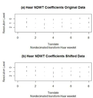
10 Example 1.2.5 of the translational invariance of the NDWT.Figure (a) depicts the NDWT Haar wavelet detail coefficients of the original data. Figure (b) depicts the NDWT Haar wavelet detail coefficients of the shifted data. Observe that the coefficients in Figure (b) are a unit shift of the coefficients displayed in Figure (a). 38

11 Stationary processes. Top: An example realisation of a white noise process (Ex-ample 1.3.3) of lengthT =1000. Bottom: An example realisation of a station-ary ARMA(2, 1) process (Example 1.3.4) of lengthT =1000 with AR parameters (α1,α2)=(0.9,−0.2) and MA parameter of 0.5. . . 41

12 Example 1.3.8: Spectral Estimationfor the realisation of an ARMA(2,1) process (Example 1.3.4) in Figure 11. Top: Raw periodogram. Bottom: Smoothed peri-odogram (using the Daniell kernel with parameterm=10). . . 43

13 The defined rhythmic parameters: periodicity, phase, amplitude and clock preci-sion (based on an image from Hanano et al. (2006)). . . 44

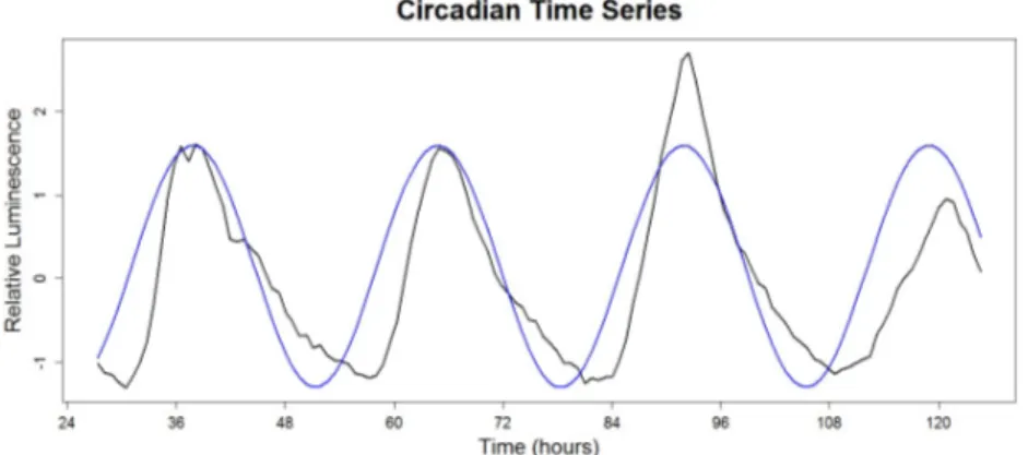
14 Example 1.3.9: Implementation of FFT–NLLS. Black line: A time series from the control group (Chapter 2); Blue line: cosine curve with period 27.03 hours (the period estimate obtained using FFT–NLLS). . . 46

15 Example 1.4.1: A time series for each of the four groups (see Chapter 2) is shown as an example– Group 1, a time series from the 100µM group; Group 2, a time series from the 150µM group; Group 3, a time series from the 200µM group. Red arrows: Plots of the estimated locations of the nonstationarities in the circadian plant signals in response to differing quantities of ammonium cerium nitrate, us-ing the wavelet spectrum test (Nason, 2013), implemented in thelocits pack-age in R which is available on CRAN. . . 49

16 Example 1.4.3. Figure (a) depicts the spectrum defined in equation (57); (b) de-picts a realisation generated from the spectrum shown in (a); (c) shows the mean of 100 uncorrected periodogram estimations computed on realisations from the spectrum shown in (a) and (d) shows the mean of 100 corrected periodogram es-timations computed on realisations from the spectrum shown in (a). Note that the spectral estimate in (d) is much closer to the true underlying spectrum than (c). 53

17 Luminescence evolution over time for plants subjected to a control and 3 differ-ent ammonium cerium nitrate concdiffer-entrations. Time is measured in hours rela-tive tozeitgebertime (time of last external temporal cue: the dawn signal of lights-on). Top left: Each plant signal from the control group (in grey) along with the group average (dashed black). Other panels: Each realisation from the groups (in grey) along with the group average and the control group average (dashed black). Group 1: 100µM ammonium cerium nitrate with average in blue. Group 2: 150µM ammonium cerium nitrate with average in green. Group 3: 200µM ammo-nium cerium nitrate with average in red. (Each time series has been normalised to have mean zero.) Note: the free run started from time 24; shaded bars below each graph indicate the subjective darkness that plants expected to experience during the ‘normal’ day. . . 56 18 Case 1.Top left: Group 1 wavelet spectrum; Top right: Group 2 wavelet spectrum;

Bottom left: Group 1 realisation and Bottom right: Group 2 realisation. . . 68 19 Case 2. Left: Group 1 wavelet spectrum (gradual period change from 24 to 25

hours); Centre: Group 2 wavelet spectrum (gradual period change from 24 to 26 hours); Right: Group 3 wavelet spectrum (gradual period change from 24 to 27 hours). . . 69 20 Case 3.Left: Group 1 wavelet spectrum (2-day transition); Centre: Group 2 wavelet

spectrum (3-day transition); Right: Group 3 wavelet spectrum (5-day transition). 69 21 Case 4.Nonstationary autoregressive processes. Top left: Estimated wavelet

spec-trum of Group 1; Top right: Estimated wavelet specspec-trum of Group 2; Bottom left: Group 1 realisation; Bottom right: Group 2 realisation. . . 70 22 Luminescence evolution over time for plants subjected to a control and 2

differ-ent copper regimes. Time is measured in hours relative tozeitgeber time (time of last external temporal cue: the dawn signal of lights-on). Centre: Each plant signal from the‘Control’group (in grey) along with the group average (dashed black). Other panels: Each realisation from the groups (in grey) along with the group average (in blue) and the control group average (dashed black). Left: ‘De-ficiency’Group (1/2 MS). Right:‘Excess’group (10µM CuSO4). (Each time series has been normalised to have mean zero.) The grey and white bars indicate the subjective night and day, respectively. . . 73 23 Results of clustering the copper dataset into two clusters using the proposed

LSW-PCA method. For each treatment group the individual signals are plotted in: red for Cluster 1 and blue for Cluster 2. The average of each treatment group is shown in black. Within each treatment group, the Cluster 1 average is shown in bold red and the Cluster 2 average in bold blue. . . 75 24 Results of clustering the copper dataset into two clusters using the proposed

LSW-PCA method. The individual signals (grey) along with the cluster average in: red for Cluster 1 and (dashed) blue for Cluster 2. . . 76 25 Cluster average estimated spectra on the copper dataset using the proposed

26 The results of clustering the cerium dataset into three groups using the proposed LSW-PCA method. The individual signals (grey) along with the cluster average in: (dashed) black for Cluster 1; blue for Cluster 2 and red for Cluster 3. The average of Cluster 1 (conceptualised as essentially ‘Control’) is shown (in dashed black) in all plots for reference. . . 79 27 Cluster average estimated spectra on the cerium dataset using the proposed

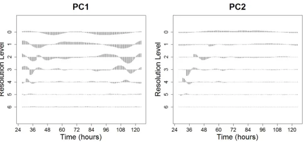
LSW-PCA method. Cluster 1 approximately corresponds to the ‘Control’ group; Cluster 2 depicts ‘Low concentration’ behaviour (100µM) and Cluster 3 the ‘Higher con-centration’ (150µM and 200µM). . . 79 28 First two principal components obtained using the proposed LSW-PCA method

on the cerium dataset. . . 80 29 The cerium dataset projected onto the first two principal components obtained

from the LSW-PCA clustering method. The colours represent the clusters: black for Cluster 1, blue for Cluster 2 and red for Cluster 3. The symbols represent the plant treatments. . . 80 30 Summary of the BRASS analysis of the circadian plant signals in response to

dif-fering quantities of ammonium cerium nitrate, represented by plots of period es-timates plotted against the respective relative amplitude errors (RAE). The colours and symbols represent the plant treatment groups: blue squares for the Control Group; green circles for Group 1 (100µM); red triangles for Group 2 (150µM) and purple stars for Group 3 (200µM). . . 83 31 Plots of the estimated locations of the nonstationarities in the circadian plant

sig-nals in response to differing quantities of ammonium cerium nitrate, using the wavelet spectrum test (Nason, 2013), implemented in thelocitspackage in R which is available on CRAN. A time series for each of the four groups is shown as an example– Group 1, a time series from the 100µM group; Group 2, a time series from the 150µM group; Group 3, a time series from the 200µM group. . . 84 32 The screeplot used to inform the selection of the number of principal

compo-nents to retain for the cerium dataset. Note 2 or 3 compocompo-nents could potentially be used, but for ease of interpretation (see Section 2.3.4.2), 2 were selected for clustering. . . 85 33 Lead dataset: Luminescence profiles over time for untreatedA. thalianaplants

(Control) and those exposed to lead nitrate (Lead). Left: Individuals in the control group (in grey) along with the group average (blue). Right: Individuals in the lead treatment group (in grey) along with the treatment group average (red) and the control group average (blue). Each time series has been standardised to have mean zero. . . 90 34 Ultradian dataset: Luminescence profiles over time for control and mutantA.

thalianaplants. Left: Individuals in the control group (in grey) along with the group average (blue). Right: Individuals in the mutant group (in grey) along with the mutant group average (red) and the control group average (blue). Each time series has been standardised to have mean zero. . . 91

35 Nematode dataset:Luminescence profiles over time for untreatedC. elegans (Con-trol) and those subjected to a pharmacological treatment (Treatment). Left: Indi-viduals in the control group (in grey) along with the group average (blue). Right: Individuals in the treatment group (in grey) along with the treatment group aver-age (red) and the control group averaver-age (blue). Each time series has been stan-dardised to have mean zero. . . 91 36 Lead dataset. Left: Average estimated spectrum of the ‘Control’ group; Centre:

Average estimated spectrum of the ‘Lead’ group; Right: ‘Barcode’ plot for FT (with FDR). . . 110 37 Ultradian dataset.Left: Average estimated spectrum of the ‘Control’ group;

Cen-tre: Average estimated spectrum of the ‘Mutant’ group; Right: ‘Barcode’ plot for HFT (with FDR). . . 111 38 Nematode dataset.Left: Average estimated spectrum of the ‘Control’ group;

Cen-tre: Average estimated spectrum of the ‘Treatment’ group; Right: ‘Barcode’ plot for FT (with FDR). . . 111 39 Q–Q plots for a representative series from the control (Plots A, C, E) and test

groups (Plots B, D, F) of each of our motivating datasets. Lead Dataset: Plots A and B. Ultradian Dataset: C and D. Nematode Dataset: E and F. . . 117 40 P1:Fixed Spectra.Top left: Group 1 wavelet spectrum; Top right: Group 2 wavelet

spectrum; Bottom left: Group 1 realisation; Bottom right: Group 2 realisation. . . 122 41 P2:Fixed Spectra-Fine Difference.Top left: Group 1 wavelet spectrum; Top right:

Group 2 wavelet spectrum; Bottom left: Group 1 realisation; Bottom right: Group 2 realisation. . . 122 42 P3:Fixed Spectra-Plus Constant.Top left: Group 1 wavelet spectrum; Top right:

Group 2 wavelet spectrum; Bottom left: Group 1 realisation; Bottom right: Group 2 realisation. . . 123 43 P4/P5: Gradual Period Change.Left: Group 1 wavelet spectrum (gradual period

change from 24 to 25 hours); Centre: Group 2 wavelet spectrum (gradual period change from 24 to 26 hours); Right: Group 3 wavelet spectrum (gradual period change from 24 to 27 hours). . . 124 44 P6: AR Processes with Abruptly Changing Parameters. Nonstationary

autore-gressive processes. Top left: Estimated wavelet spectrum of Group 1; Top right: Estimated wavelet spectrum of Group 2; Bottom left: Group 1 realisation; Bottom right: Group 2 realisation. . . 125 45 P7: AR Processes with Slowly Changing Parameters.Top left: Estimated wavelet

spectrum of Group 1; Top right: Estimated wavelet spectrum of Group 2; Bottom left: Group 1 realisation; Bottom right: Group 2 realisation. . . 126 46 P10: ‘Function Plus Noise’ Time Series with Constant Period. Top left:

Esti-mated wavelet spectrum of Group 1 (24 hour period); Top right: EstiEsti-mated wavelet spectrum of Group 4 (23 hour period); Bottom left: Group 1 realisation; Bottom right: Group 4 realisation. Grey lines indicate a 24 hour period. . . 126

47 DEFRA Chemicals: Luminescence profiles over time forA. thalianaplants ex-posed to a selection of the DEFRA chemicals. Each Panel: Individuals in the chemical treatment group (in grey) along with the treatment group average (red) and the control group average (blue). Each time series has been standardised to have mean zero. . . 138 48 DEFRA Chemicals: Luminescence profiles over time forA. thalianaplants

ex-posed to a selection of the DEFRA chemicals. Each Panel: Individuals in the chemical treatment group (in grey) along with the treatment group average (red) and the control group average (blue). Each time series has been standardised to have mean zero. . . 140 49 Mercury (Max):Luminescence profiles over time for untreatedA. thalianaplants

(denoted ‘Control’) and those exposed to mercuric chloride (HgCl2) at a concen-tration of 5µM (denoted ‘Mercury (Max)’). Left: Individuals in the control group (in grey) along with the group average (blue). Right: Individuals in the Mercury (Max) treatment group (in grey) along with the treatment group average (red) and the control group average (blue). Each time series has been standardised to have mean zero. . . 143 50 ‘Barcode’ plotsfor FT (with FDR) for the time series shown in Figure 47. . . 145 51 ‘Barcode’ plotsfor FT (with FDR) for the time series shown in Figure 48. . . 146 52 Periodic tables, coloured by effect on the circadian clock ofA. thaliana

(Oaken-full et al., 2018).A: Coloured by FFT-NLLS period estimates (red outlines indicate a statistically significant change in period for all compounds tested).B: Coloured by percentage change from control using FT (FDR) analysis. AandB: Green ele-ments are essential to life and were not tested individually; White eleele-ments were not tested due to safety or solubility. The actinoids and group 7 elements have been omitted as they were not tested. . . 149 53 Time series and Barcode plots for Strontium, Platinum and Rubidium. Time

series (left panels): Blue lines indicate the control average for each chemical; grey lines indicate individual time series within each chemical treatment group and red lines indicate the average time series for the chemical treatment group. Bar-code plots (right panels): BarBar-code plots for FT (with FDR) at the 5% significance level. . . 150 54 Time series and Barcode plots for Gold, Tungsten and Lutetium. Time series

(left panels): Blue lines indicate the control group average for each chemical; grey lines indicate individual time series within each chemical treatment group and red lines indicate the average time series for the chemical treatment group. Bar-code plots (right panels): BarBar-code plots for FT (with FDR) at the 5% significance level. . . 151

55 Ruthenium: Luminescence profiles over time for untreatedA. thaliana plants (denoted ‘Control’) and those exposed to ruthenium chloride (RuCl3) at a con-centration of 2mM (denoted ‘Ruthenium’). Left: Individuals in the control group (in grey) along with the group average (blue). Right: Individuals in the Ruthe-nium treatment group (in grey) along with the treatment group average (red) and the control group average (blue). Each time series has been standardised to have mean zero. . . 153 56 DEFRA Chemicals (plate 0953):Luminescence profiles over time forA. thaliana

plants exposed to a selection of the DEFRA chemicals. Each Panel: Individuals in the chemical treatment group (in grey) along with the treatment group average (red) and the control group average (blue). Each time series has been standard-ised to have mean zero. . . 156 57 The results of clustering the DEFRA Chemicals (plate 0953) into 2 groups using

the LSW-PCA method. The individual signals (grey) along with the cluster average in: red for Cluster 1 and blue for Cluster 2. The individual signals of the Lead (Max) treatment group in Cluster 1 are plotted in green. . . 157 58 DEFRA Chemicals (plate 0952):Luminescence profiles over time forA. thaliana

plants exposed to a selection of the DEFRA chemicals. Each Panel: Individuals in the chemical treatment group (in grey) along with the treatment group average (red) and the control group average (blue). Each time series has been standard-ised to have mean zero. . . 164 59 The results of clustering the DEFRA Chemicals (plate 0952) into 3 groups using

the LSW-PCA method. The cluster average time series in: red for Cluster 1 (con-ceptualised as ‘Cadmium (Max)’); blue for Cluster 2 (con(con-ceptualised as ‘Arsenic (Max)’) and green for Cluster 3 (conceptualised as ‘Arsenic (Half )’). . . 165 60 The results of clustering the DEFRA Chemicals (plate 0952) into 3 groups using

the LSW-PCA method. The individual signals of the modal treatment group (grey) along with the cluster average in: red for Cluster 1; blue for Cluster 2 and green for Cluster 3. For each cluster, the individual signals in the non–modal treatment group are plotted in: red for Cadmium (Max); blue for Arsenic (Max) and green for Arsenic (Half ). . . 166

Introduction

The earth rotates on its axis every 24 hours resulting in a day and night cycle. Correspondingly, almost all species exhibit changes in their behaviour between day and night (Bell-Pedersen et al., 2005). These daily rhythms are not only caused by a response to daily changes in the physical environment, but are also the result of an internal timekeeping system or ‘biological clock’ within the organism (Vitaterna et al., 2001; Minors and Waterhouse, 2013). In partic-ular, most plants are able to anticipate dawn and adjust their biochemistry accordingly. The mechanisms underlying the biological timekeeping systems, and the potential consequences of their failure, are among the issues addressed by researchers in the field of circadian biology (McClung, 2006; Bujdoso and Davis, 2013).

Circadian rhythms are a subset of biological rhythms with a period of approximately 24 hours. The term ‘circadian’ (derived from the Latin words “circa” (about) and “dies”(day)) was first used by Franz Halberg in the 1950s (McClung, 2006). Furthermore, a defining attribute of circadian rhythms is that they are “endogenously generated and self-sustaining” (McClung, 2006). In other words, they are the result of an internal timekeeping system–“endogenously generated”– and the period remains approximately 24 hours under constant environmental conditions, such as constant light (or dark) and constant temperature (i.e. when deprived of any external time cues)– “self-sustaining”.

The first recorded observations (in western literature) of circadian rhythms appeared in the fourth century BC, when Androsthenes described the daily leaf movements of the tamarind tree (McClung, 2006). However, at the time it was assumed that these movements were due to the plant reacting to the day-night cycle (not the result of an internal clock) and it took over 2000 years for these observations to be experimentally tested. The first instance of scientific litera-ture on circadian rhythms was in 1729 when the French astronomer de Mairan discovered that the daily leaf movements of certain plants persisted in constant darkness. This demonstrated for the first time that the plant could not be reacting to the external cues associated with a light–dark cycle, potentially indicating the existence of an internal timekeeping system. How-ever, these experiments did not take temperature into account and it took a further 30 years before de Mairan’s observations were independently repeated (in constant darkness) with con-stant ambient temperature (McClung, 2006). Almost 100 years later, the period length of these leaf movements was accurately measured and shown to be onlyapproximately24 hours. The result that the rhythms were not exactly 24 hours was crucial as it provided evidence that these rhythms were driven by an internal timekeeping system and not simply responses to an unde-tected geophysical cue associated with the rotation of the earth on its axis (such as light leaking into the laboratory darkroom!)

However, leaf movement is only one among many circadian rhythms in plants that include: germination; growth; enzyme activity; stomatal movement and gas exchange; photosynthetic activity; flower opening and fragrance emission (McClung, 2006). Therefore, in the 1970s, re-searchers began using genetic analysis with the intention of: identifying components of circa-dian clocks and elucidating the oscillator mechanism central to the circacirca-dian clock in a number of organisms, including the laboratory model plant speciesArabidopsis thaliana. These early experiments were quite labour intensive, but advances in experimental methods in the 1990s meant that relative gene expression could be quantifiedin vivo(Plautz et al., 1997; Southern

and Millar, 2005; Perea-García et al., 2016a). Experiments recording plant response to light entrainment (constant light) result in datasets that, from a statistical point of view, can be con-sidered as time series realisations.

Time series are ubiquitous and their analysis has found important applications in, for ex-ample, economics, climatology and, of course, circadian biology. For series that satisfy certain properties, such as stationarity (i.e. statistical properties such as the mean and variance are as-sumed constant over time) there are well—established methods of statistical analysis which are classically based on Fourier representations (see for example Priestley (1982); Shumway and Stoffer (2000); Brillinger (2001); Percival and Walden (2006) for an introduction to the topic). This thesis is concerned with analysis methods for nonstationary time series. In particular, we address a number of applied problems in the field of circadian biology, where nonstationar-ity is common (Zielinski et al., 2014) and replicate information is available. Access to replicate information, though standard in many biological applications, is atypical for time series data. Consequently, there is a gap in the current time series literature. In this thesis, we are primarily interested in clustering nonstationary time series and also determining if two (groups of ) time series differ in terms of their spectral structure, and, if so, how?

Wavelets can be thought of as localised, oscillatory basis functions with several attractive properties for function representation. They are localised in both time and frequency, provid-ing sparse multiscale representations for many signals. Due to their time localisation, wavelets provide natural ‘building blocks’ for nonstationary series. In this thesis, we develop clustering and hypothesis testing procedures based on wavelets.

This thesis is structured as follows: Chapter 1 provides an overview of aspects of the litera-ture which are essential to the work subsequently developed. In particular, we give an overview of basis representations and an introduction to wavelet theory including the discrete wavelet transform (DWT). We then introduce the topic of stationary time series analysis, and its rele-vant applications in circadian biology. We also review the current state-of-the-art period es-timation methods for circadian data. We then describe various approaches to nonstationary time series analysis and, in particular, the locally stationary wavelet (LSW) model of Nason et al. (2000), which provides the modelling framework for the methodology developed in Chapters 2 and 3 .

The work in Chapter 2 is motivated by the phenomenon of individual-level variability in plant response to stimuli, despite their sharing identical genetic characteristics (Doyle et al., 2002). The presence of multiple nonstationary behaviours within the same experimental treat-ment group motivates the developtreat-ment of a clustering procedure that can detect these different characteristics and analyse them separately, whilst accounting for nonstationarity. Hence, in Chapter 2, we develop and test (both through an extensive simulation study and application to a previously published circadian dataset) a new method for clustering rhythmic biological data. The proposed methodology combines locally stationary wavelet time series modelling with functional principal components analysis and thus extracts the time-scale patterns aris-ing in a range of rhythmic data. Interestaris-ing and encouragaris-ing results are obtained by applyaris-ing the clustering methodology to a newly–generated circadian dataset. Nevertheless, the devel-oped methodology has wider applicability; it can be applied to other circadian datasets, as well as to data originating in other fields.

treat-ment has caused a significant change in a rhythmic biological signal. When these signals dis-play nonstationary behaviour, the established methodologies may be misleading. Therefore, in this chapter, we develop new methodology that enables the formal comparison of nonstation-ary processes. As circadian behaviour is best understood in the spectral domain (Hargreaves et al., 2018), we develop novel hypothesis testing procedures in the (wavelet) spectral domain, embedding replicate information when available. Motivated by three complementary appli-cations in circadian biology, our new methodology allows the identification of three specific types of spectral difference. We demonstrate the advantages of our methodology over alterna-tive approaches, by means of a comprehensive simulation study and real data applications, us-ing both published and newly generated circadian datasets. In contrast to the current standard methodologies, our proposed method successfully identifies differences within the motivat-ing circadian datasets, and facilitates wider rangmotivat-ing analyses of rhythmic biological data. This demonstrates the utility of the proposed methodology, which again is not restricted to these applications.

Throughout this thesis, our work is motivated by a specific application in the field of cir-cadian biology– the effect of industrial and agricultural pollutants on the plant circir-cadian clock (Foley et al., 2005; Senesil et al., 1998; Hargreaves et al., 2018; Nicholson et al., 2003). Specifi-cally, the Department for Environment, Food and Rural Affairs (DEFRA) developed ‘Soil Guide-line Values’ (SGVs) that can be used to determine appropriate concentrations of certain chem-icals in soil. Therefore, in Chapter 4, we apply the wavelet spectral testing and clustering methodologies developed within this thesis to investigate the impact of exposure to the chem-icals at the concentrations outlined in the DEFRA report, as well as to chemchem-icals not included in the report, on the plant circadian clock. Our findings indicate that many of the tested chem-icals have an effect on the plant circadian clock. Therefore, the results of Chapter 4 could be used to inform a revision of the SGVs. Thus, the results of Chapter 4 not only have important implications for understanding environmental ramifications associated with soil pollution, but also demonstrate the additional insight gained by using the appropriate methodologies, as de-veloped in Chapters 2 and 3.

Finally, Chapter 5 concludes with a summary of our work and some interesting ideas for future research.

Acknowledgements

First and foremost my thanks go to my team of supervisors: Marina Knight, Jon Pitchford and Seth Davis. A few people questioned the wisdom of having three voices, but I think we proved them wrong! Thank you Jon for being the maths–biology translator! Also thank you for your support and kindness and sense of humour (which was so often needed)! Thank you Seth for your generosity with your time, all your useful/ useless (delete as appropriate) facts and all the conversations about American sports and Eurovision! And thank you to Marina Knight (always right). I have nominated her for supervisor of the year every year for the last four years! But, due to the fact that I never threatened to quit my PhD (which of course is down to their excellent supervision), she is yet to win the award! Marina, you are an inspiration on a personal and professional level. And look– I went a whole paragraph without writing “in particular” or “therefore”! You have taught me so much!

Thanks also go to Agostino Nobile for being an excellent and very helpful Thesis Advisory Panel. I cannot apologise enough for the 40 page TAP reports that arrived 2 days before meet-ings! Also, thank you for all your time and patience when we worked together lecturing Stats 2. I wouldn’t be where I am without that experience and you were there every step of the way.

Also thank you to all members of the Davis Lab. The lessons I have learnt through pre-senting and listening at the weekly lab meetings have been invaluable. Special mentions to: Jack; Kayla (one of the kindest people I have ever met); Mandi (Go Tribe!) and Rachael (without which none of the work in this thesis would have been possible). I wish all of you the best in your future endeavours.

Finally, I want to thank my family for much more than words can ever say. Mainly, proof reading and counselling! And generally putting up with me in work–mode for the past four years.

Declaration

I declare that this thesis is a presentation of original work and that I am the sole author, under the supervision of Dr. Marina Knight, Dr. Jon Pitchford and Prof. Seth Davis. Unless specified otherwise (see below), I performed all literature research, programming, analysis and writing of the thesis chapters. Under the supervision of Dr. Marina Knight, Dr. Jon Pitchford and Prof. Seth Davis, I developed and implemented the statistical methodology in Chapters 2 and 3. The novel circadian datasets analysed in this thesis were obtained by the Davis and Chawla Labs (Biology, University of York).

This work has not previously been presented for an award at this, or any other, University. All sources are acknowledged as References.

The following chapters of the thesis have been published in or submitted to peer–reviewed journals. I am the first author on two of the three papers, but have received feedback and corrections from my co–authors.

0.1 Chapter 2

The novel circadian dataset analysed in this chapter was obtained by the Davis Lab (Biology, University of York). The BRASS analysis of this dataset was performed by R. Oakenfull.

This chapter has been published as:

Hargreaves, J. K., Knight, M. I., Pitchford, J. W., Oakenfull, R. and Davis, S. J. (2018). Clus-tering nonstationary circadian plant rhythms using locally stationary wavelet representations. SIAM Multiscale modeling and simulation, 16(1):184–214.

0.2 Chapter 3

The novel ‘Lead dataset’ analysed in this chapter was obtained by the Davis Lab (Biology, Uni-versity of York). The BRASS analysis of this dataset was performed by R. Oakenfull. The novel ‘Nematode dataset’ analysed in this chapter was obtained by the Chawla Lab (Biology, Univer-sity of York). The BRASS analysis of this dataset was performed by J. Munns.

This chapter has been submitted for publication to the Annals of Applied Statistics as: Hargreaves, J. K., Knight, M. I., Pitchford, J. W., Oakenfull, R., Chawla, S., Munns, J. and Davis, S. J. (2018). Wavelet spectral testing: application to nonstationary circadian rhythms. arXiv preprint arXiv:1803.09507.

0.3 Chapter 4

The novel circadian dataset analysed in this chapter was obtained by the Davis Lab (Biology, University of York). The BRASS analysis of this dataset was performed by R. Oakenfull. I per-formed the wavelet spectral testing and produced the resulting figures.

The results and discussion of the BRASS analysis and wavelet spectral testing are in prepa-ration for publication (with R. Oakenfull as the lead author) as:

Oakenfull, R., Hargreaves, J. K., Knight, M. I., Pitchford, J. W. and Davis, S. J. (In Preparation). Out of the sewage rises new maths...

In Chapter 4, I present the results of the above analyses. However, I selected which of the above results to discuss in detail and wrote the text of the thesis chapter (with feedback and

guidance from my supervisors). I also performed the cluster analysis (which is not included in the manuscript in preparation).

1 Literature Review

This chapter provides an overview of aspects of the literature which are essential to the work presented in this thesis. Section 1.1 gives an overview of basis representations and Section 1.2 gives a more detailed introduction to wavelet theory. Section 1.3 introduces the topic of stationary time series analysis, and, in particular, Section 1.3.2 its applications in circadian biology (which motivated the work in this thesis), as well as reviewing the current state-of-the-art period estimation methods for circadian data. Finally, Section 1.4 describes approaches to nonstationary time series analysis and, in particular, the locally stationary wavelet model. 1.1 Basis Representations

We begin by first reviewing some relevant concepts from Fourier analysis. An understanding of these methods provides the motivation for the use of wavelets, since certain signals cannot be represented efficiently using the trigonometric functions which form the basis of Fourier analysis. Fourier methods also underpin some of the commonly used period estimation meth-ods for circadian data (see Section 1.3.2) and provide the benchmark for comparison with the (wavelet-based) methodology we develop in later chapters.

Our review of Fourier analysis follows the description in Priestley (1982) and the review of wavelet theory synthesises the descriptions in Daubechies (1992), Vidakovic (1999) and Nason (2010). We refer the reader to these texts for a more detailed discussion.

1.1.1 Fourier Analysis

In classical Fourier analysis, trigonometric functions (i.e. sine and cosine waves) are used to form the bases for functions in the space ofsquare integrable functions,

L2(R)=nf |

Z ∞

−∞|

f(t)|2d t< ∞o.

We define the Fourier series representation of a function,f, as follows.

Definition 1.1.1. Let f be periodic (with period 2π) and square integrable over the interval [0, 2π). Then theFourier seriesrepresentation of f is:

f(x)=a0 2 + X n∈Z+ ³ ancos(nx)+bnsin(nx) ´ ,

where the Fourier coefficients are calculated from

an= 1 π Z 2π 0 f(x) cos(nx)d x, bn= 1 π Z 2π 0 f(x) sin(nx)d x.

The Fourier coefficients, an andbn in Definition 1.1.1, are calculated using theL2inner

product. The magnitudes of the Fourier coefficients provide information about the frequency composition of the signal. The Fourier functions, {cos(nx), sin(nx)}n∈N, form an orthonormal basis and can be thought of as the “building blocks” from which certain periodic functions can be constructed.

However, most functions are not periodic. The Fourier transform is an extension of the Fourier series in that it provides a representation of non-periodic functions in the space of

absolutely integrable functions,

L1(R)=©g|

Z _∞

−∞|

g(t)|d t< ∞ª.

The trigonometric “building blocks” of the Fourier series in Definition 1.1.1 are replaced by complex exponentials in the definition of the Fourier (and inverse Fourier) transform.

Definition 1.1.2. TheFourier transformof a function g∈L1(R)is given by ˆ g(ω)=p1 2π Z Rg(x) exp −iωx_{d x} .

Ifg is the Fourier transform of g andˆ gˆ,g∈L1(R), then theinverse Fourier transformis given by g(x)=p1

2π

Z

Rgˆ(ω) exp

iωx_{dω. (1)}

Note that in the Fourier integral representation, frequency varies on a continuous scale, as opposed to the Fourier series decomposition which involves a discrete set of frequencies.

1.1.1.1 Sampling and Aliasing

In many practical applications, a discrete series is obtained by sampling a continuous function at equal intervals,∆t. For a sampling interval∆t >0 and an arbitrary time offsett0, we can define a discrete process through

Xt≡X(t0+t∆t),

for t =0,±1,±2, . . . . The frequency 1/(2∆t) is called the Nyquist frequency (or folding quency) and defines the highest frequency that can be seen in discrete sampling. Higher fre-quencies sampled in this way will appear at lower frefre-quencies calledaliases(Shumway and Stoffer, 2000).

Example 1.1.3. In this example, we demonstrate the effect of aliasing by sampling from two different cosine curves (one at the Nyquist frequency and one over this value) at equal inter-vals∆t =1. The results can be seen in Figure 1. In Figure 1, the dashed lines represent the underlying (continuous) functions from which we are sampling. The dashed black line rep-resents a cosine curve with a frequency of 1/(2∆t)=0.5 (i.e. the Nyquist frequency) and an amplitude of 2. This function makes a cycle every two time units, therefore, the value of each observation of this function is zero (the black circles, Figure 1). The dashed blue line repre-sents a cosine curve with a frequency of 1=2×1/(2∆t) (i.e. double the Nyquist frequency) and an amplitude of 2. This function makes a cycle every time unit, therefore, the value of each observation of this function is also zero. This demonstrates how sampling the function with the higher frequency in this way would give the same results as sampling the function at the Nyquist frequency (known as aliasing).

Example 1.1.4. In Chapter 2, we analyse a dataset taken from a broad investigation of the effect of various salt stresses on the plant circadian clock. In this experiment, measurements were taken at intervals of approximately 45 minutes. Therefore, the Nyquist frequency (the highest

Figure 1: Example 1.1.3. Dashed black line: Underlying cosine curve with a frequency of 1/(2∆t)=0.5 (i.e. the Nyquist frequency) and an amplitude of 2; Dashed blue line: Underly-ing cosine curve with a frequency of 1=2×1/(2∆t) (i.e. double the Nyquist frequency) and an amplitude of 2; Black circles: Observed value of underlying functions att=1, 2, . . . , 5.

frequency that can be seen in discrete sampling) is 1 2∆t = 1 2×0.75= 2 3, which is equivalent to a period of 1.5 hours.

1.1.1.2 Discrete Fourier Transform

We can now define the discrete Fourier transform as follows.

Definition 1.1.5. Given data X1, . . . ,Xnwe define thediscrete Fourier transform (DFT)to be

d(ωj)= 1 p n n X t=1 Xtexp−2πiωjt (2)

for j=0, 1, . . . ,n−1, where frequenciesωj=j/n are called theFourierorfundamental

fre-quencies.

Example 1.1.6. In this example, we create a simple time series, and then demonstrate how we can extract the frequency information using Fourier analysis. The time series is the sum of two underlying cosine curves: the first at a frequency of 6/128 with an amplitude of 2 and the second at a frequency of 10/128 with an amplitude of 4:

X(t)=2 cos µ 2πt 6 128 ¶ +4 cos µ 2πt 10 128 ¶ . (3)

The underlying cosine curves and resulting time series (sampled att=1, . . . , 128) are shown in Figure 2. The (squared) DFT (called the periodogram– also see Section 1.3.1 later) is also plotted in Figure 2. Note that the periodogram is only non–zero at the frequencies 6/128 and 10/128 and the value of the periodogram at these values is equal to the amplitude of the corresponding

Figure 2:Example 1.1.6. Top left: First underlying cosine curve with a frequency of 6/128 and an amplitude of 2; Top right: Second underlying cosine curve with a frequency of 10/128 and an amplitude of 4; Bottom left: The time series is a linear combination of two underlying cosine curves (see equation (3)); Bottom right: raw periodogram of the series with the frequencies 6/128 and 10/128 indicated by vertical red lines and horizontal green lines indicating values of 4 and 16 (which correspond to the amplitudes of the underlying cosine components squared– see equation (3)).

underlying cosine curve squared. Therefore, the periodogram has correctly determined the underlying frequencies of our time series.

Example 1.1.7. In this example, we modify the time series from Example 1.1.6 such that the period of the series abruptly changes. The time series is now the concatenation of the above two underlying cosine curves:

X(t)=        2 cos µ 2πt₁₂₈6 ¶ , t∈[1, 128]. 4 cos µ 2πt₁₂₈10 ¶ , t∈(128, 256]. (4)

The underlying cosine curves (sampled att=1, . . . , 128), resulting time series (sampled att= 1, . . . , 256) and periodogram are shown in Figure 3. Note that the periodogram is almost identi-cal to the periodogram in Figure 2. Therefore, this analysis has identified the periodicity of the data, however, it cannot detect changes of period through time. Such changes are common in many biological systems (see Section 1.3.2) and will call for more sophisticated methodology, able to cope with time–varying periods and amplitudes.

When representing a series by a combination of basis functions, it is usually desirable that the representation is sparse (i.e. there are only a small number of non-zero coefficients). This is because a sparse representation can aid understanding of the signal structure. Furthermore, a sparse representation also leads to better signal compression. In other words, we would prefer to represent a large number of data points by a much smaller number of basis coefficients in-stead. Sparse decompositions can be achieved by using basis functions with similar properties to the function that is being represented. Fourier functions are localised in frequency but not in time. Therefore, Fourier functions are suitable for representing smooth, periodic functions,

Figure 3: Example 1.1.7. Top left: First underlying cosine curve with a frequency of 6/128 and an amplitude of 2; Top right: Second underlying cosine curve with a frequency of 10/128 and an amplitude of 4; Bottom left: The time series is the concatenation of the two cosine curves (see equation (4)); Bottom right: raw periodogram of the series with the frequencies 6/128 and 10/128 indicated by vertical red lines and horizontal green lines indicating values of 4 and 16 (which correspond to the amplitudes of the underlying cosine components squared– see equation (4)).

but are not as suitable for functions with local features such as sharp changes and disconti-nuities. In order to represent such functions, we would prefer basis functions that have short support i.e. are localised in time. One solution is to use wavelets, which are described in the next section.

1.1.2 Wavelet Representations

The name “wavelet” gives us a clue as to two important properties of wavelets: this word ap-pears to describe a “little wave” (as opposed to a “big wave” such as the trigonometric functions in Fourier theory). A “wavelet” can thus be thought of as a small, localised wave. This property makes it an ideal candidate to represent functions with local features (which proved problem-atic for the Fourier functions above). Formally, as in Daubechies (1992) we define a wavelet as follows.

Definition 1.1.8. Awaveletis any square integrable function,ψ∈L2(R)which satisfies the ad-missibility condition, C_ψ= Z R |_ψˆ(ω)|2 |ω| dω< ∞, (5)

where_ψˆ(ω)is the Fourier transform ofψ(x)(see definition 1.1.2). The admissibility condition (5) implies

Z _∞

−∞ψ

(x)d x=0, (6)

which ensures its oscillatory behaviour (Vidakovic, 1999).

A wavelet basis can be formed bytranslatinganddilatinga basis function called themother wavelet, which we will denoteψ(x). In this thesis, we focus on wavelet functions whose dyadic

dilations and translations form an orthonormal basis ofL2(R). Formally, the collection of func-tions {ψj,k}j,k∈Z, defined by:

ψj,k(x)=2

j

2ψ₍₂j_{x−k), (7)}

known as adiscrete (decimated) wavelet family, forms an orthonormal basis ofL2(R). The functionsψj,k(x) in equation (7) are the wavelets generated by the motherψ. Informally, this

demonstrates that once the “type” of wavelet has been chosen and fixed (in this case, theψ function) we can now generate other wavelets by transforming the mother wavelet. In partic-ular, we can generate wavelets (in our case, theψj,k’s) by dilating and translating the mother

wavelet. In fact, the parametersjandkin equation (7) are known as thedilationand transla-tion parametersrespectively. The dilation parameter indicates the wavelet scale (see section 1.2.1) and the translation parameter indicates the location. The wavelet family then forms an orthonormal basis ofL2(R) and is analogous to the sine and cosine functions used in Fourier analysis.

When for eachk∈{0, . . . ,m}, we have

Z ∞

−∞

xkψ(x)d x=0, (8)

the waveletψin equation (8) is said to havem+1vanishing moments. The vanishing moments property of a wavelet implies that the wavelet coefficients of polynomials of degreemor less are zero in a decomposition on such a wavelet basis. Therefore, this property has important implications when selecting a wavelet basis that would give a sparse representation of a given function.

Example 1.1.9. The Haar Basis.The simplest wavelet is theHaar wavelet(see Figure 4) and we discuss it as an introductory example throughout this review. The Haar wavelet is commonly used to introduce the topic of wavelets due to its simplicity, yet it displays many characteristic features of wavelets.

The Haar mother wavelet is a mathematical function,ψH:R→{±1, 0}, defined by

ψH_(x) =          1, ifx∈[0, 1/2). −1, ifx∈[1/2, 1). 0, otherwise. (9)

Using equation (7), the translations forj,k∈Zof the Haar mother wavelet are given by

ψH j,k(x)=            22j, ifx∈ h k 2j,₂kj+₂j1+1 ´ . −22j, ifx∈ h k 2j+₂j1+1, k 2j+₂1j ´ . 0, otherwise. (10)

and example plots for various values ofjandkare given in Figure 4.

As in Fourier analysis, we can use wavelet functions as a basis to represent other functions. Recall (above) that dilations and translations of a mother wavelet functionψ(x) (ie. ψj,k)

de-fine an orthonormal basis inL2(R). Throughout this thesis, we will consider only real–valued wavelet functions, therefore, we define the wavelet representation of a functionf as follows.

Figure 4: Panel (a): Haar mother wavelet. Panels (b), (c), (d): translations and dilations of the Haar mother wavelet (using equation (10) for various combinations ofj=1, 2 andk=1, 2).

Definition 1.1.10. Given a function f ∈L2(R), itswavelet representationis given by f(x)= ∞ X j=−∞ ∞ X k=−∞ dj,kψj,k(x), (11)

where, due to the orthogonality of wavelets, for j,k∈Z: dj,k=

Z ∞

−∞

f(x)ψj,k(x)d x=<f,ψj,k>, (12)

where< ·,· >is the L2-inner product.

The numbers {dj,k}j,k∈Zare referred to as thewavelet coefficientsof f. As for the Fourier coefficients discussed in Section 1.1.1, the wavelet coefficients also provide information about the structure of the function, f. However, we note that the Fourier coefficients only provide information about the amplitude associated with each frequency, whereas the wavelet coeffi-cients provide information about the amplitude of the wavelet at both a given (time) location and scale (associated with frequency, see Section 1.2.1).

1.2 Wavelet Theory

1.2.1 Multiresolution Analysis

A common way of introducing wavelet bases and demonstrating their properties is to con-struct them within the framework of a multiresolution analysis (MRA), introduced by Mallat