Published SFF-8414 Rev 10.1

(1)

SFF Committee documentation may be purchased in hard copy or electronic form. SFF specifications are available at ftp://ftp.seagate.com/sff

SFF Committee

SFF-8414 Specification for

HPEI Passive Cable Assembly and PCB S-Parameter Measurements

Rev 10.1 January 24, 2007

Secretariat: SFF Committee

Abstract: This specification defines the requirements for measuring S-Parameters that are suitable for accurate characterization of passive HPEI cable assemblies and PCB’s in the speed range that is compatible with test equipment and test fixtures that are available today. Such cable assemblies are used in most applications requiring high speed serial and serial-parallel electrical connections. HPEI is an acronym for high performance electrical interconnect.

This specification provides a common specification for systems manufacturers, system integrators, and suppliers of magnetic disk drives. This is an internal working document of the SFF Committee, an industry ad hoc group.

This document is made available for public review, and written comments are solicited from readers. Comments received by the members will be considered for inclusion in future revisions of this document.

The description of a test procedure in this specification does not assure that the specific hardware necessary for executing the procedure is actually available from instrumentation suppliers. If such hardware is supplied it must comply with this specification to achieve interoperability between suppliers.

Support: This document is supported by the identified member companies of the SFF Committee.

POINTS OF CONTACT:

Bill Ham I. Dal Allan

Editor Chairman SFF Committee 92 Wildwood Road 14426 Black Walnut Court Andover, MA 01810 Saratoga CA 95070

Ph: 978-828-9102 Fx: 978-475-8315 Ph: 408-867-6630 Fx: 408-867-2115 Email: [email protected]

(2)

EXPRESSION OF SUPPORT BY MANUFACTURERS

The following member companies of the SFF Committee voted in favor of this industry specification. Amphenol EMC FCI Fujitsu CPA Hewlett Packard Hitachi GST LSI Logic Molex Samsung Sun Microsystems Tyco AMP Vitesse Semiconductor

The following member companies of the SFF Committee voted to abstain on this industry specification. AMCC Brocade Clariphy Comax Cortina Systems Emulex Foxconn JDS Uniphase Seagate Sumitomo Toshiba America

The user's attention is called to the possibility that implementation to this

Specification may require use of an invention covered by patent rights. By distribution of this Specification, no position is taken with respect to the validity of this claim or of any patent rights in connection therewith. The patent holder has filed a

statement of willingness to grant a license under these rights on reasonable and non-discriminatory terms and conditions to applicants desiring to obtain such a license.

(3)

Foreword

The development work on this specification was done by the SFF Committee, an industry group. The membership of the committee since its formation in August 1990 has included a mix of companies which are leaders across the industry.

When 2 1/2" diameter disk drives were introduced, there was no commonality on external dimensions e.g. physical size, mounting locations, connector type, connector location, between vendors.

The first use of these disk drives was in specific applications such as laptop portable computers and system integrators worked individually with vendors to develop the

packaging. The result was wide diversity, and incompatibility.

The problems faced by integrators, device suppliers, and component suppliers led to the formation of the SFF Committee as an industry ad hoc group to address the marketing and engineering considerations of the emerging new technology.

During the development of the form factor definitions, other activities were suggested because participants in the SFF Committee faced more problems than the physical form factors of disk drives. In November 1992, the charter was expanded to address any issues of general interest and concern to the storage industry. The SFF Committee became a forum for resolving industry issues that are either not addressed by the standards process or need an immediate solution.

Those companies which have agreed to support a specification are identified in the first pages of each SFF Specification. Industry consensus is not an essential requirement to publish an SFF Specification because it is recognized that in an emerging product area, there is room for more than one approach. By making the documentation on competing proposals available, an integrator can examine the alternatives available and select the product that is felt to be most suitable. SFF Committee meetings are held during T10 weeks (see www.t10.org), and Specific Subject Working Groups are held at the convenience of the participants. Material presented at SFF Committee meetings becomes public domain, and there are no restrictions on the open mailing of material presented at committee meetings.

Most of the specifications developed by the SFF Committee have either been incorporated into standards or adopted as standards by EIA (Electronic Industries Association), ANSI (American National Standards Institute) and IEC (International Electrotechnical

Commission).

If you are interested in participating or wish to follow the activities of the SFF Committee, the signup for membership and/or documentation can be found at:

www.sffcommittee.com/ie/join.html

The complete list of SFF Specifications which have been completed or are currently being worked on by the SFF Committee can be found at:

ftp://ftp.seagate.com/sff/SFF-8000.TXT

If you wish to know more about the SFF Committee, the principles which guide the activities can be found at:

ftp://ftp.seagate.com/sff/SFF-8032.TXT

Suggestions for improvement of this specification will be welcome. They should be sent to the SFF Committee, 14426 Black Walnut Ct, Saratoga, CA 95070.

(4)

SFF Committee --

HPEI Passive Cable Assembly and PCB S-Parameter Measurements

1. Scope

The SFF Committee was formed in August, 1990 to broaden the applications for storage devices, and is an ad hoc industry group of companies representing system integrators, peripheral suppliers, and component suppliers.

2. References

The SFF Committee activities support the requirements of the storage industry, and it is involved with several standards.

2.1 Industry Documents

The following interface standards are relevant to many SFF Specifications. - X3.131R-1994 SCSI-2 Small Computer System Interface

- X3.253-1995 SPI (SCSI-3 Parallel Interface) - X3.302-xxxx SPI-2 (SCSI-3 Parallel Interface -2) - X3.277-1996 SCSI-3 Fast 20

- asd;LAKJ PIP (Passive Interconnect Performance)

- X3.221-1995 ATA (AT Attachment) and subsequent extensions

- EIA PN-3651 Detail Specification for Trapezoidal Connector 0.50" Pitch used with Single Connector Attach -2.

- X3.230-1994 FC-PH (Fibre Channel Physical Interface) and subsequent extensions FC-PH-3, FC-PI, FC-PI-2, FC-PI-3 and FC-PI-4 - ANSI-Y14.5M Dimension and Tolerancing

- MIL-STD-1344, Method 3008 Shielding Effectiveness of Multicontact Connectors. - IEC 96-1, Reverberation Chamber method for measuring the screening

effectiveness of passive microwave components. 2.2 SFF Specifications

There are several projects active within the SFF Committee. The complete list of

specifications which have been completed or are still being worked on are listed in the specification at ftp://ftp.seagate.com/sff/SFF-8000.TXT

2.3 Sources

Those who join the SFF Committee as an Observer or Member receive electronic copies of the minutes and SFF specifications (http://www.sffcommittee.com/ie/join.html).

Copies of ANSI standards may be purchased from the InterNational Committee for Information Technology Standards (http://tinyurl.com/c4psg).

Copies of SFF, T10 (SCSI), T11 (Fibre Channel) and T13 (ATA) standards and standards still in development are available on the HPE version of CD_Access

(http://tinyurl.com/85fts).

2.4 Conventions

The American convention of numbering is used i.e., the thousands and higher multiples are separated by a comma and a period is used as the decimal point. This is equivalent to the ISO/IEC convention of a space and comma.

American: ISO: 0.6 0,6 1,000 1 000

(5)

TABLE OF CONTENTS 1. Scope ... 4 2. References ... 4 2.1 Industry Documents ... 4 2.2 SFF Specifications ... 4 2.3 Sources ... 4 2.4 Conventions ... 4 3. Description ... 7

4. General statement of application space for this document ... 7

4.1 Physical components and frequency ranges ... 7

4.2 Uses of S-parameters ... 8

4.2.1 Overview... 8

4.2.2 Pass/fail schemes... 8

4.2.3 Summary... 10

5. Definitions ... 10

6. Framework for S-parameter measurements ... 11

6.1 General concept of S-parameters ... 11

6.1.1 Overview... 11

6.1.2 Theoretical requirements for S-parameters at the measurement system interface ... 13

6.2 Basic S parameter signal measurement definitions ... 13

6.3 Definition of S parameter naming conventions ... 14

6.3.1 IUT port identification... 14

6.3.2 Extension to a 2-pair IUT... 15

6.4 Coverage of the S-parameter matrix ... 17

6.4.1 Theoretical coverage... 17

6.4.2 Practical issues relating to coverage... 17

6.5 Relationship between frequency domain and time domain instrumentation ... 19

6.5.1 General relationships... 19

6.5.2 Mapping between S-parameters and time domain measurements... 20

6.5.3 Practical full coverage comparison for time domain and frequency domain methods 21 6.6 Documentation of the S-parameter file ... 23

6.6.2 Documentation of a single pair IUT file... 23

6.6.3 Documentation of a 2-pair IUT file... 25

6.7 Partial coverage of the S-parameter matrix ... 27

6.7.2 Main variables in determining coverage cost... 29

7. Identification of the IUT ... 29

7.1 Overview ... 29

7.2 Physical IUT boundary description ... 29

7.3 Reference plane ... 30

7.4 Examples of reference planes and IUT boundaries ... 31

8. Accounting for the test fixture in S-parameter measurements ... 33

8.1 Overview ... 33

8.2 Extraction of S-parameters from a practical measurement ... 34

9. Basic measurement requirements ... 36

9.1 General ... 36

9.2 Measurement instrumentation ... 36

9.2.2 Definition of instrumentation type... 37

9.2.3 Calibration of instrumentation... 37

9.2.4 TDNA resolution and bandwidth considerations... 37

9.2.5 VNA (frequency domain) set-up considerations... 38

(6)

9.3.2 Test fixture and associated calibration structure design... 38

9.4 Measurement procedures ... 44 9.4.1 Overview... 44 9.4.2 SOLT method... 45 9.4.3 TRL method... 46 9.4.4 De-embedding... 46 9.4.5 Normalization method... 46

(7)

3. Description

This document is about creating accurate and transportable S-parameter measurements on physical interconnect cable assemblies and PCB’s (termed IUT for Interconnect Under Test). Many features of using S-parameters impact the testing or measurement process so a description of what S-parameters are and what is involved with creating a complete set of S-parameters for IUT’s of interest is included.

This technology appears deceptively simple yet is truly mathematically elegant in its ability to describe very complex behaviors.

Use of S-parameters is becoming more widespread as different standards seek practical ways to specify complex signal performance without requiring ‘golden’ hardware and to mitigate the challenges of making accurate waveform measurements at very high

frequencies. Previously there has not been a significant demand for transportable S-parameter files as most uses were for design. However, when using S-S-parameter based methods for compliance to standards and for using S-parameter based methods to allow accurate simulation of complex waveforms, the transportability property rises to the forefront.

This work complements other work in the T11 (Fibre Channel) committee under the signal modeling (FCSM-2) and signal performance specification (MSQS) projects by taking a pragmatic view of the measurement portion.

This document covers three broad areas:

• Thorough description of S-parameters and the general requirements for attaining adequate coverage

• Specifies the format for transporting S-parameter files, including the formats for transporting cross talk and other pair to pair (more than four single ended ports) interaction measurements.

• Specifies acceptance criteria for determining whether calibration structures accurately represent the test fixture.

This document does not provide detailed step-by-step instructions for making

calibrations or measurements because these are usually determined by the specific test equipment and its related calibration software. The test equipment and software

manufacturers provide calibration, test method step-by-step instructions, and application notes.

The procedures described in this document are not optimized for high volume production testing. They are primarily intended for use as reference methods that can resolve disputes and deliver adequate accuracy for use in compliance testing and simulation.

4. General statement of application space for this document

4.1 Physical components and frequency ranges

Physical implementations are passive cable assemblies up to 15 meters long, PCB based interconnects, and the compliance interconnects (both cable and PCB based) used by various standards to verify transmitter device compliance. The lower length limits are determined by the properties of the S parameter measurement set up (typically around one cm).

Signals used in the end application are between 1 GBaud and 12.75 GBaud serial NRZ stream (800 Mb to ~10 Gb/s using 8b10b encoding). The higher the frequency range for the S parameters the more complete the S-parameter description of the IUT properties an

(8)

the more difficult the problem of obtaining transportable S-parameters. The methods described in this document are suitable for a frequency range of up to 20 GHz based on fundamental considerations required to generate eye diagrams using the S-parameter measurements with a suitable simulation tool.

These constraints lead to requirements on the frequency step size that depends on the length such that the frequency step causes less than 360 degree phase change.

See clause 6 for the explanation of the insertion loss and return loss terms used in the following paragraphs.

Insertion loss type measurements are assumed to have at least – 60 dB noise floor with lower floors attainable without excessive effort. This noise floor is well below the range of interest (around – 40 dB)

Return loss type measurements are expected to have values in the neighborhood of -10 dB at 9 GHz. A noise floor for return loss measurements of better than -20 dB is required at 9 GHz to achieve adequate accuracy for product characterization.

There is a belief that there is a fundamental challenge to making adequate return loss measurements in the 10 GHz range and this is the reason for the relatively high return loss target. Insertion loss measurements under these conditions appear to be

reasonably attainable using well known methods and equipment.

4.2 Uses of S-parameters

4.2.1 Overview

The purpose of this document is to ensure that the basic measurement of the

S-parameters adequately and accurately captures the behavior of the IUT and that these measurement results can be accurately repeated on the same IUT by other laboratories. The S parameters measured for the IUT after removal of the test fixture contributions can be used for a number of purposes. One use is as a model of the behavior of the IUT without any concept of pass or fail. Other uses may involve specifying pass-fail

criteria. The modeling/characterization use is straightforward. The pass/fail uses, however, are a subject of significant controversy in the industry.

Once the complete set of S-parameters are known for an IUT one may calculate or simulate waveform responses for the IUT. The properties of these waveforms may be criticized for compliance. Some standards choose to place limits on the values of the S-parameters themselves and others use a mixture of waveform properties and S-parameter values for compliance.

4.2.2 Pass/fail schemes 4.2.2.1 Overview

There are two pass/fail schemes in common use that are discussed in this clause. Both require the use of simple limit masks but one mask is specified in the time domain and the other mask is specified in the frequency domain. Masks can be arbitrarily complex and in the theoretical limit both methods yield equivalent results. In practice, however, the need for having simple masks drives significant differences between these pass-fail methods.

(9)

4.2.2.2 Time domain masks

One pass-fail scheme for S-parameter files is in creating eye diagrams or other

simulated time domain responses by using a simulation tool with the S-parameter file as part of the simulation input. Pass or fail is indicated by whether the simulated

signal violates a time domain limit mask (eye or other type of mask). This use appropriately indicates the suitability of the IUT for a specific signal without any over or under specification.

A different time domain mask is required for each behavior tested. For output differential signals an eye mask that may not be crossed is often used. By using multiple launched signals at different ports the combined effects of cross talk can be included in the output differential signals. For output common mode signals staying below a specified maximum time domain amplitude limit may be all that is required. For reflected signals a TDR type of time domain limit mask may be used.

However, just because a specific S-parameter file passes the time domain mask test for a particular signal with a set of properties does not automatically mean that some other signal with a different set of properties will also pass the time domain limit mask test with that same IUT. If the IUT is to be used for a range of applications then multiple signals, each representing a specific set of conditions within the allowed range of applications, are required to determine compliance for the IUT.

4.2.2.3 Frequency domain masks

The other pass-fail scheme for S-parameter files is to place a frequency domain limit mask directly on individual S-parameter files. Each different parameter has a

different mask. If any specific S-parameter for the IUT exceeds its respective mask then the IUT fails. This pass-fail methodology is generally significantly over-conservative and does not allow for any trade-offs between parameters.

For example, an insertion loss suckout at some frequency may be perfectly fine if there is little frequency content in the signal at that frequency. But the insertion loss limit mask would probably fail the perfectly good IUT (for that signal).

In another example an IUT might have better insertion loss but more cross talk and the two parameters trade off to yield a good IUT. A limit mask would fail the good IUT (for that signal) for high cross talk.

A benefit of the limit mask approach is that if the complete set of (simple) limit masks for all S-parameters for the IUT can all be met then it is likely that the IUT will work for a fairly broad range of applications. It may require significant cost increases or design constraints for the IUT to meet this set of requirements.

4.2.2.4 Closed eyes

It is worth noting that closed eyes on differential signals that may be seen at the end of lossy links are no problem for using the eye mask scheme for pass-fail purposes. With closed eyes one must simply apply a reference receiver to the signals before applying the eye diagram acceptance criteria (mask). The reference receiver processes the signal in a specified and standard way such that the processed eye is open. Such reference receivers are being specified in a number of standards and also have the benefit that they allow the link signal budget (jitter/amplitude etc.) to attain ‘credit’ for the signal processing done in receivers that process the signal (for example using equalization). Having a closed eye going into the reference receiver is not a valid reason to require the use of limit masks on the individual S-parameters.

(10)

4.2.3 Summary

It is not the purpose of this document to recommend which method should be used for compliance purposes as each has benefits and drawbacks. One key drawback to using limits on S-parameter values is the tendency to over specify performance; local deviations over a small frequency range may not harm the application. Engineering tradeoffs cannot easily be incorporated into the acceptance limits because there is no relationship to the actual application requirements. One key benefit to using the s-parameter limit method is ease of implementation without needing a signal simulation tool.

5. Definitions

Bilateral: the ability of an IUT to remain invariant in all electrical properties upon end to end reversal of the IUT. Bilaterality is only possible if the connectors on the IUT have the same design.

Calibration - the process of removing instrumentation errors at a specific point in the system called the reference plane, which may be located as shown in Figure 13 and

Figure 14 in 8414 depending on the method. Use of known standards and/or defined reference structures is required.

Calibration enabling structure – Special structures required in the instrumentation calibration process

De embedding – the process of removing test fixture effects by using matrix algebra where the Sij of the test fixture is known.

Instrumentation – the collection of hardware and software that is used to excite and detect signals applied to or detected from the reference plane used during the IUT measurement. Instrumentation may or may not include test fixtures depending on the method used. Instrumentation may or may not include internal calculations.

IUT – Interconnect under test

Normalization: a term used to describe a process of accounting for the test fixture insertion losses for the magnitude of the IUT insertion loss and for the phase effect of the test fixtures. This process is only accurate for test fixtures that produce no reflections.

Reciprocal: the property of having identical waveshapes at the receiver and transmitter if the position of the transmitter and receiver are reversed. Often the impedance of the transmitter and receiver make it impractical to access the points in the system where the ideal transmitter and receiver exist. Waveshapes determined only by the insertion loss properties are generally reciprocal even when the connectors are different on each end of the IUT if the transmitter and receiver impedance are

identical as required for S-parameter measurement. Even though IUT’s with different connectors have the same insertion loss in either direction (i.e., S21=S12) this same IUT will not have the same return loss on either end and therefore is not bilateral. The return loss is, however, still reciprocal even in the presence of unequal

reflections on both ends of the IUT because by definition the transmitter and the receiver are at the same place on the same end for return loss. And the IUT is also reciprocal even with unequal return loss because the total effect of the reflections is the same at the ports even though the losses occur at different places in the two

directions.

Reference plane: a defined location in the physical setup where measurements are assumed to apply. Formally reference planes require TEM (Transverse ElectroMagnetic) transmission mode (where the electric and magnetic fields are both perpendicular to the direction of propagation) at the reference plane. This assumption is often not

(11)

satisfied due to practical physical constructions of connectors. Only very high

quality straight transmission lines offers close to actual TEM conditions. The coaxial construction is the closest. Within a PC board a straight trace is another example. Non TEM constructions and imperfections in the construction are sources of measurement error that cannot be fully corrected. In addition to practical design constraints of making TEM structures there is an error source because a fixture without the IUT does not have the same construction or imperfections as when the IUT is attached. Errors from this source all have higher order propagation modes as the root cause.

SOLT - short open load thru; an acronym for a set of defined steps for calibrating and removing the effects of the test fixture. This process involves sequentially measuring the properties of the test fixture under different conditions of special short, open, load, and thru connections in place of the IUT. A separate set of calculations using these results is required to account for the test fixture in the IUT measurement.

Symmetry – having identical properties with respect to a defined point, line, or plane. Symmetry requires a modifier to be unambiguous. For example, mirror symmetry describes an object whose reflection with respect to a plane is identical to the object. Other types may include: end to end, rotational, axial, etc.

Test fixture – the exact same hardware (same trace, same wire, same connector etc.) that is used to physically connect to the IUT. The test fixture may or may not be part of the instrumentation depending on the method.

Test fixture characterization structure – Special structures used to allow removal of the test fixture effects from the measurement.

Time domain gating - a process of using only information the time domain response in the time region where the IUT exists

TRL - thru, reflect, line; an acronym for a set of defined steps for calibrating and removing the effects of the test fixture. This process involves building a special calibration test fixture that is ‘identical’ to the test fixture to be used with the IUT. This special test fixture has structures that emulate the thru, reflect, and line conditions. A separate set of calculations using these results is required to account for the test fixture in the IUT measurement.

6. Framework for S-parameter measurements

6.1 General concept of S-parameters

6.1.1 Overview

S-parameters or scattering parameters are one of many possible ways to represent the behavior of a linear system. S-parameters are the ratio of the output amplitude to the input amplitude and the difference between the output phase and the input phase.

Equivalently the real and imaginary properties of the respective signals may be used. In S-parameters the signal description includes the propagation direction. Thus it is possible to have an S-parameter for a single port by relating the reflected signal to the incoming signal.

S-parameters assume a perfect resistive termination (e.g., most systems use 50 ohms single ended, 100 ohm differential) is attached to all ports. This includes active ports where the signal is applied (signal source has perfect source impedance), the response port where the signal is measured and any ‘not connected’ ports that are not being used for the measurement. As such, S-parameters measurements are intrinsically

(12)

‘laboratory’ measurements. The reference impedance for the S-parameter shall be explicitly stated if not 50 ohms single ended or 100 ohms differential.

While S-parameters can be measured for a single frequency their utility is limited to IUT properties only at that frequency. Since IUT’s are called on to transport complex data patterns and waveforms that contain a wide range of frequencies it is necessary to examine S-parameters across the range of frequencies that are important to the end use application. When the term ‘S-parameter’, or one of the specified symbols that

identify the S-parameter, is used in this document it refers to the entire set of

properties across the frequency range and is actually a large number of discrete values that individually describe the signal level (or sinusoidal signal amplitude, rms or dB), the phase, and the frequency.

S parameters are defined by a subscript system where the first numerical subscript defines the port number for the outbound response signal from the IUT and the second numerical subscript defines the port number for the applied incident signal to the IUT. The applied incident signal is always propagating into the IUT and the outbound

response signal is always propagating out of the IUT.

It is not sufficient to only describe an S-parameter by the two numbered port subscripts because both differential and common mode signals may be described by S-parameters. The basic terminology is ‘D’ for differential and ‘C’ for common mode. Maintaining the convention that the first subscript always describes the outbound response signal from the IUT and the second subscript always describes the applied incident signal into the IUT, a four subscript convention results, SABij.

For example S_DC14defines the ratio of the differential signal coming out of differential port 1 to the common mode signal applied at differential port 4. To avoid the

inconvenience of creating, accommodating, and reading small subscripts the ‘subscripts’ are often raised to full font characters added after the letter ‘S’. For example, the S_DC14 could also be written as SDC14.

If no ‘D’ or ‘C’ is present then it is assumed that the signals are single ended. It is common to calculate differential and common mode S-parameters from the measured single ended responses to single ended applied signals.

The port numbering scheme and the IUT description scheme can be complex as discussed in 6.3. The port numbering scheme shall be clearly specified in the description of the IUT in all cases.

Regardless of whether an S-parameter port is single ended or differential (two single ended ports per differential port) the description of the IUT defines the port

numbering. For example, an IUT could have differential port 1 consisting of single ended port 1 and single ended port 3. In this case the IUT access points have multiple accurate numbering – one set for the differential ports and another set for the single ended ports.

However, even if only differential ports are assigned numbers is it still necessary to separately identify each leg of the differential pair so that the common mode and mode conversion properties are captured.

Differential port identification is usually assigned according to the single ended port pairs connected to a single wire pair (e.g., twisted pair or twinax) in the IUT.

However, mathematically, S-parameters allow assignment of differential ports to

arbitrary pairs of single ended ports. If the full S-parameter set is measured for the IUT then all the information for the IUT will be in the results. It may require

careful mapping of ports numbers to actual construction to make much sense of the data unless an intelligent port numbering scheme is used up front.

(13)

6.1.2 Theoretical requirements for S-parameters at the measurement system interface A reference plane is defined as the location in the physical setup where measurements are assumed to apply. The formal definition of a reference plane requires TEM

(Transverse ElectroMagnetic) transmission (where the electric and magnetic fields are both perpendicular to the direction of propagation) at the reference plane. This assumption is often not satisfied due to practical physical constructions of

connectors. Only very high quality straight transmission lines offers close to actual TEM conditions. The coaxial construction is the closest. Within a PC board a straight trace is another example. Non TEM constructions and imperfections in the construction are sources of measurement error that cannot be fully corrected. In addition to

practical design constraints of making TEM structures there is an error source because a fixture without the IUT does not have the same construction or imperfections as when the IUT is attached. Errors from this source all have higher order propagation modes as the root cause.

6.2 Basic S parameter signal measurement definitions

Figure 1 shows the connections, 1, 2, 3, and 4, made to a four port instrument such as a vector network analyzer (VNA) or a time domain network analyzer (TDNA) for measuring S parameters on a four single ended port ‘black box’ device. Such a device could be a single differential pair in an IUT. The instrumentation recognizes signals going into the ‘black box’ denoted by the ‘a’ subscript and signals coming out of the ‘black box’ denoted by the ‘b’ subscript. These instruments may do this separation via directional couplers, for example, but how they do it is not part of this document. S-parameters use only the voltages with the a and b subscripts since propagation direction is required to be known. In the absence of directional separation the total voltage, V_i, is observed.

All the measurements specified in this document relate to differential signal pairs. It requires all four single ended instrumentation ports to measure the properties of two differential ports.

Instrumentation ports may be single ended with the differential and common mode properties for differential ports calculated, typically internal to the instrument. Some instruments may also directly measure and detect differential and/or common mode signals. No instruments are presently known that extract the single ended behaviors from differential and common mode measurements.

(14)

Figure 1 - Architecture of a 4 port measurement (single ended measurements)

6.3 Definition of S parameter naming conventions

6.3.1 IUT port identification

Subclause 6.1 defined the general naming conventions but there is another dimension to this topic, namely, defining specifically which port gets which number for a real IUT. There is general agreement that the downstream side of the IUT for normal signal flow in service is generally assigned the higher differential port numbers. The single ended port numbering may not follow this rule rigorously but usually the highest single ended port number will be on the downstream side and the lowest single ended port

number will be on the upstream side. So for identification of ports with numbers the problem is straightforward – simply make sure that the following information is

provided:

• The DD,CC,DC,CD, or none for single ended, conventions are used for all data • A clear picture of the IUT is provided with the file that shows which connector

contact (or contacts for differential) belongs to which port number

• A statement of the normal signal flow direction in service for the IUT being measured.

There are several other legitimate port identification schemes in use. Figure 2 shows five different schemes each following a logical (but different) pattern.

When the S-parameter files are finally created a numbering scheme shall be used in the file so a translation between the contact naming scheme used for the physical IUT and the port numbering scheme used in the data file must be done and clearly documented.

“PHYSICAL BLACK BOX”

1

2

4

3

V

2

V

3

V

4 GROUND REFERENCE “MATHEMATICAL BLACK BOX”

1

2

4

3

V

₁

= V

_a1

+ V

_b1

V

a1

V

b1

V

_a2

V

b2

V

a4

V

_b4

V

a3

V

b3

Numbers are used to identify terms in this figure and do

not represent requirements on port numbering in general

(15)

Figure 2 - Different schemes used for identifying IUT ports

This document does not require any specific port identification or port numbering scheme for the physical IUT but compliance with this document does require that the three bulleted items above be delivered with the S-parameter data files that apply to the IUT. It is worth noting that the In+, In-, Out+, Out- scheme provides the best overall independence from specific service application and specific measurement method. The signal flow direction and the differential sense are explicitly defined. Since some IUT’s may not directly connect to transmitter devices or receiver devices the Tx,Rx scheme is less desirable.

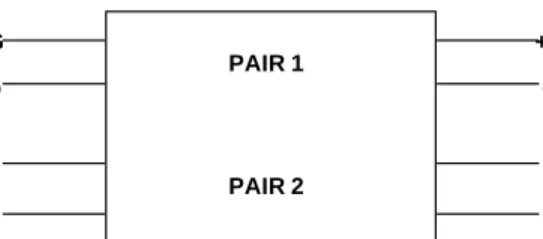
6.3.2 Extension to a 2-pair IUT

Figure 3 shows the definition of the differential ports and the

differential-to-differential S parameters that may be acquired from a two pair IUT. If using a four single ended port instrument only two differential ports may be measured at one time. The physical reconfiguration required to access all the differential S parameters listed in Figure 3 is shown in Figure 4.

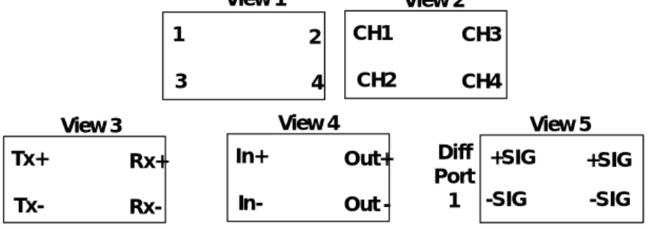
IUT port (pinout) identification conventions – five equivalent views:

View 1: IUT ports are identified according to the VNA port numbering scheme (Agilent numbers shown, other numbers may be used for other instruments) View 2: IUT ports are identified according to the TDNA channel numbering

scheme

View 3: IUT ports are identified according to the function provided by the device that is connecting to the IUT in normal service

View 4: IUT ports are identified according to the signal flow through the IUT View 5: IUT ports are identified according to SFF-84xx conventions using +SIG and –SIG and differential port numbering

Single pair IUT

1 2 4 3 View 3 Tx+ Rx+ Rx- Tx-View 4 In+ Out+ Out - In-View 1 View 2 CH1 CH4 CH2 CH3 View 5 +SIG +SIG -SIG -SIG Diff Port 1 Diff Port 2

(16)

Figure 3 - Definition of differential-to-differential S parameters

In Figure 3 a partial mapping between the S-parameter names and the common verbal descriptions that may be used is given.

In general for the SABij shown in Figure 3:

• If i=j, and A=B then the parameter is a RETURN LOSS (going into and out of the

same port with the same mode in and out)

• If i j, and A=B then the parameter is an INSERTION LOSS between ports i and j for

the same mode in and out.

However for the special cases where the same wires are not connected

between ports i and j in the IUT then this type of insertion loss is called CROSS TALK

Cross talk is NEAR END when ports i and j are on the same end of the IUT and FAR END when ports i and j are on the opposite ends of the IUT

• If A B (not shown in Figure 3) then the parameter is a MODE CONVERSION

CAUTION: S-PARAMETERS ARE A MEASURE OF GAIN (OUTPUT REFERRED TO INPUT) BY DEFINITION. HOWEVER COMMON USAGE HAS INCORRECTLY IMPLEMENTED THE WORD ‘LOSS’ INSTEAD OF GAIN. PARAMETERS WHOSE AMPLITUDE IS EXPRESSED AS A NEGATIVE DB VALUE REPRESENT A GAIN LESS THAN ONE OR A POSITIVE ‘LOSS’. PLEASE EXERCISE CAUTION IN THIS AREA AND UNDERSTAND THAT DATA MAY BE PRESENTED OR LABELED INCORRECTLY (i.e, GAINS BEING LABELED AS LOSSES).

Figure 3 and Figure 4 list only the differential-to-differential S-parameters (SDDij).

The common mode-to- common mode (SCCij), the common mode-to-differential (SDCij), and the differential-to common mode (SCDij) are also required for creating the complete set of 64 S-parameters for the IUT.

+ SIG - SIG DIFF PORT 1 DIFF PORT 4 DIFF PORT 3 DIFF PORT 2 PAIR 1 PAIR 2

SDD11 = DIFFERENTIAL RETURN LOSS FROM DIFF PORT 1 SDD22 = DIFFERENTIAL RETURN LOSS FROM DIFF PORT 2 SDD33 = DIFFERENTIAL RETURN LOSS FROM DIFF PORT 3 SDD44 = DIFFERENTIAL RETURN LOSS FROM DIFF PORT 4

SDD21 = DIFFERENTIAL INSERTION LOSS AT DIFF PORT 2 FROM DIFF PORT 1 SDD31 = DIFFERENTIAL NEAR END CROSS TALK AT DIFF PORT 3 FROM DIFF PORT 1 SDD41 = DIFFERENTIAL FAR END CROSS TALK AT DIFF PORT 4 FROM DIFF PORT 1 SDD42 = DIFFERENTIAL NEAR END CROSS TALK AT DIFF PORT 4 FROM DIFF PORT 2 SDD43 = DIFFERENTIAL INSERTION LOSS AT DIFF PORT 4 FROM DIFF PORT 3 SDD32 = DIFFERENTIAL FAR END CROSS TALK AT DIFF PORT 3 FROM DIFF PORT 2 SDD34 = DIFFERENTIAL NEAR END CROSS TALK AT DIFF PORT 3 FROM DIFF PORT 4 SDD12 = DIFFERENTIAL INSERTION LOSS AT DIFF PORT 1 FROM DIFF PORT 2 SDD13 = DIFFERENTIAL NEAR END CROSS TALK AT DIFF PORT 1 FROM DIFF PORT 3 SDD14 = DIFFERENTIAL FAR END CROSS TALK AT DIFF PORT 1 FROM DIFF PORT 4 SDD23 = DIFFERENTIAL FAR END CROSS TALK AT DIFF PORT 2 FROM DIFF PORT 3 SDD24 = DIFFERENTIAL NEAR END CROSS TALK AT DIFF PORT 2 FROM DIFF PORT 4

+ SIG - SIG + SIG - SIG + SIG - SIG

(17)

6.4 Coverage of the S-parameter matrix

6.4.1 Theoretical coverage

For an N-port IUT a complete set of all S-parameters is required to fully represent the behavior of the IUT. For an IUT with N differential ports this includes:

SDDij SCCij SDCij SCDij

where both i and j are the differential port numbers and both i and j are fully and independently varied from 1 to N to cover all of the differential ports on both ends of the IUT.

It requires a lot of work and time to measure a full S-parameter set even if the IUT is only as complex as two differential pairs. Even in this ‘simple’ 2-pair case, it

requires an 8-port single ended instrument to access all the single ended ports with a single IUT physical connection. The practical limit for most instruments is a single differential pair (that requires 4 single ended ports).

For the simple one pair case where N = 2 there are four single ended ports (two per pair). Let us temporarily call these single ended ports 1+, 1-, 2+ and 2- where the number is the number of the differential port and the + - is the leg of the pair. Each single ended port requires four frequency sweeps to cover all the cases where that single ended port is the source. So if single ended port 1+ is the source the complete set is S1+1+, S2+1+, S1-1+, S2-1+. Each port must act as source in turn so it requires 16 sets of single ended data to completely populate the S-parameter matrix for an IUT with a single pair. Fortunately, most 4-port instruments available today automatically connect the appropriate source, measure at the appropriate output and keep track of all the data that results.

It should be even more obvious at this point that clear port numbering is VITAL. For a 2-pair IUT having 8 single ended ports and using an 8 port (single ended) instrument the number of frequency sweeps is 64. The general formula is:

Number of frequency sweeps = (2N)2

= (4P)2

where N is the number of differential ports and P is the number of pairs in the IUT. See also 6.7 for discussion of partial coverage.

6.4.2 Practical issues relating to coverage

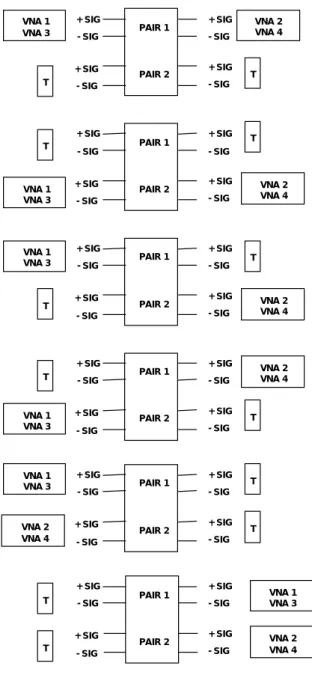
Figure 4 shows all the test configurations required for measurement of a complete

S-parameter set for a 2-pair IUT when using a 4-port instrument. Although Figure 4 shows the connections for a VNA, the same information may be obtained by using time domain measurements to acquire time domain waveforms. Practical coverage of a two-pair IUT with a 4 port instrument requires 6 different IUT connections with 6 different sets of 4 port measurement results. Note that termination is required on all differential ports that are not connected to the instrument during the measurement.

Post processing of the 6 data sets is required to assemble the complete S-parameter set for the 2-pair IUT into a single matrix set.

In Figure 4 only the SDDij are specifically called out. The SCCij, SCDij, and SDCij

(18)

Figure 4 - Test configurations required when using a 4-port VNA or TDNA instrument with a 2-pair IUT DIFF PORT 1 DIFF PORT 4 DIFF PORT 3 DIFF PORT 2 + SIG - SIG + SIG - SIG DIFF PORT 1 DIFF PORT 4 DIFF PORT 3 DIFF PORT 2 + SIG - SIG + SIG - SIG DIFF PORT 1 DIFF PORT 4 DIFF PORT 3 DIFF PORT 2 + SIG - SIG + SIG - SIG DIFF PORT 1 DIFF PORT 4 DIFF PORT 3 DIFF PORT 2 + SIG - SIG + SIG - SIG DIFF PORT 1 DIFF PORT 4 DIFF PORT 3 DIFF PORT 2 + SIG - SIG + SIG - SIG DIFF PORT 1 DIFF PORT 4 DIFF PORT 3 DIFF PORT 2 PAIR 1 PAIR 2 PAIR 1 PAIR 2 PAIR 1 PAIR 2 PAIR 1 PAIR 2 PAIR 1 PAIR 2 PAIR 1 PAIR 2 + SIG - SIG + SIG - SIG + SIG - SIG + SIG - SIG + SIG - SIG + SIG - SIG + SIG - SIG + SIG - SIG + SIG - SIG + SIG - SIG + SIG - SIG + SIG - SIG + SIG - SIG + SIG - SIG TERMINATOR VNA 1 VNA 3 T T T VNA 2 VNA 4 VNA 1 VNA 3 VNA 2 VNA 4 T T T T T T T T T T VNA N VNA or TDNA PORTS

VNA PORTS ARE SINGLE ENDED SOURCES ARE ASSUMED AS VNA 1 AND VNA 3

RECEIVERS ARE ASSUMED AS VNA 2 AND VNA 4

THE FUNCTION OF THE VNA PORTS AS SOURCES OR RECEIVERS ARE CONTROLLED BY THE VNA INTERNALLY FOR SDDnn RETURN LOSS MEASUREMENT THE VNA PROVIDES THE FAR END TERMINATION INTERNALLY TO THE VNA

PAIR 1 ONLY SDD11, SDD12, SDD21, SDD22 PAIR 2 ONLY SDD33, SDD34, SDD43, SDD44

PAIR 1 AND PAIR 2 FAR END INTERACTIONS CONFIGURATION 1

SDD14, SDD41

SDD32, SDD23

PAIR 1 AND PAIR 2 NEAR END INTERACTIONS CONFIGURATION 3

SDD31, SDD13

PAIR 1 AND PAIR 2 NEAR END INTERACTIONS CONFIGURATION 3 SDD42, SDD24 IUT NOMENCLATURE 4 PORT VNA NOMENCLATURE PAIR 1 ONLY SDD11, SDD12, SDD21, SDD22 PAIR 2 ONLY SDD11, SDD12, SDD21, SDD22 VNA 1 VNA 3 VNA 2 VNA 4 VNA 2 VNA 4 VNA 2 VNA 4 VNA 2 VNA 4 VNA 1 VNA 3 VNA 1 VNA 3 VNA 1 VNA 3 PAIR 1 AND PAIR 2

FAR END INTERACTIONS CONFIGURATION 1

SDD12, SDD21

SDD12, SDD21

(19)

An 8-port instrument would be better than the 4-port instrument shown because there are intrinsic inefficiencies and risks listed below that are built into doing the multiple IUT connections shown in Figure 4:

• Every IUT needs to be connected and reconnected to the instrumentation multiple times – this is not only time consuming but every connection and reconnection action moves the IUT, may damage the IUT and takes time • The instrumentation may lose calibration while executing the full

coverage measurements

• There is an increased chance of connection error due to multiple connections

• There is an increased chance of data mismanagement since several complex data sets are produced and must be recombined later to form the overall S-parameter file set for the IUT

• There are a multiplicity of measurements that are duplicated. All the measurements into and out of the same port and all the measurements across the same differential port in both directions is duplicated 8 times in the example used in Figure 4.

In the case shown in Figure 4 there are 6 measurement configurations each with 16 frequency sweeps for a total of 6 X 16 = 94 frequency sweeps collected. There are also 8 cases where ports are measured into and out of and across themselves that were also measured elsewhere. In each of these cases 4 frequency sweeps were recorded. When these redundant measurements are

accounted for we end up with 96 – 32 = 64 unique frequency sweeps which is the same as that for the 8-port instrument that did not have the duplications. However, there may be value in this duplication in that one can compare these supposedly redundant frequency sweeps to determine how repeatable the

measurements are and whether the assumptions of ‘perfect’ termination on all ports was satisfied.

Clearly there are many IUT’s that have more than two differential pairs. The amount of testing, data management, and post processing required for complete coverage goes up roughly as N2

with the pair count. So there is a practical consideration with the measurement of S-parameters of how much of the complete S-parameter set is necessary to measure and how much can be ‘assumed’. The issues associated with executing a reduction in coverage are discussed more fully in sub-clause 6.7.

6.5 Relationship between frequency domain and time domain instrumentation

6.5.1 General relationships

This sub-clause defines the relationship between the measurement types involved.

The frequency domain measurements excite and detect the properties of sine waves at a single frequency. Multiple frequencies are measured in a sweep across a defined frequency range. The time domain measurements excite and detect waveforms. The waveforms contain all the signal level, frequency, and phase information found in the frequency domain methods though in a different form. These waveforms may then be converted to S parameters using a suitable software package typically using a version of Fourier transforms. Similarly the frequency domain measurements contain all the time domain waveform

information.

If the time domain waveform is excited and detected from the same port it is called a time domain reflection measurement or TDR. If the waveform is

(20)

excited at one port and detected at another port it is call a time domain transmission measurement or TDT. Time domain measurements involve comparing the differences between the excited and detected waveforms.

6.5.2 Mapping between S-parameters and time domain measurements

The following three figures contain 4 x 4 matrices that show all the

differential, common mode, and mode conversion S parameters that are possible from a differential 2-port (single ended 4 port) IUT. The kind of time domain measurements used to create the specific kind of frequency domain S parameters is shown with the double headed arrows.

In Figure 5 the differential only portions are shown in larger font. In Figure 6 the common mode only portions are shown in larger font. In Figure 7 the mode conversion responses are shown in larger font. Transmission

responses acquired via TDT and reflection responses acquired via TDR are noted.

Return loss uses TDR methods. Insertion loss (including cross talk) and mode conversion uses TDT methods.

For differential measurements differential stimulus signals are used with differential response measurements. For common mode measurements common mode stimulus signals are used with common mode response measurements. For mode conversion measurements differential stimulus with common mode response or common mode stimulus with differential response is used.

Figure 5 – Differential TDR stimulus, differential response

Figure 6 – Common mode TDR stimulus, common mode response

CC22

TDR

S

TDT

S

TDT

S

TDT

S

TDT

S

TDR

S

TDT

S

TDR

S

TDR

S

TDR

S

TDT

S

TDR

S

↔

CC22 CC21 CC21 CD22 CD22 CD21 CD21 CC12 CC12 CC11 CC11 CD12 CD12 CD11 CD11 DC22 DC22 DC21 DC21 DC12 DC12 DC11 DC11

TDR

S

TDT

S

TDT

S

TDR

S

DD22

DD21

DD12

DD11

↔

TDT

S

TDT

S

TDT

S

TDR

S

TDR

S

TDR

S

TDR

S

TDT

S

TDT

S

TDR

S

TDT

S

TDR

S

CD22 CD22 CD21 CD21 CD12 CD12 CD11 CD11 DC22 DC22 DC21 DC21 DD22 DD21 DD21 DC12 DC12 DC11 DC11 DD12 DD12 DD11 DD11

↔

Common mode TDR stimulus, common mode response

TDR

S

TDT

S

TDT

S

TDR

S

CC22

CC21

CC12

CC11

↔

DD22

(21)

Figure 7 – Mixed mode, two cases shown in one matrix for convenience

6.5.3 Practical full coverage comparison for time domain and frequency domain methods

Some practical time domain instruments are capable of directly measuring and detecting differential and common mode signals as well as the single ended signals. These time domain instruments produce full coverage with a different set of measurements than frequency domain instruments.

The number of measurements required for full coverage (frequency sweeps or waveform captures) is the same for both frequency domain and time domain. There are 16 measurements required for a 1-pair IUT. This applies whether single ended or differential signals are used by the instrument. However, the time to collect the data may be significantly less with the time domain

because the time domain instruments use real time waveforms while the swept frequency methods use a ‘lock and roll’ technique where each frequency is locked on using an IF detector and measured separately before rolling to the next frequency.

The time required for frequency domain frequency sweeps is determined mostly by the number of frequency points required which in turn is determined by the application.

The number of frequency points required is specified in several places. For example, for bulk cable testing SFF-8416 specifies how to determine the number of frequency points. The Fibre Channel FCSM-2 document has requirements

applying to signal modeling applications. Others probably exist in other standards and industry documents. Compliance with SFF-8414 requires implementing the properties specified following in this sub-clause unless otherwise specified in other application documents.

Compliance with the following requirements

• Assures that any insertion loss suckouts and return loss and cross talk

peaks will be detected with good resolution

• Assures that the electrical length (defined immediately below) and phase

content is adequately represented for the IUT – no missing points due to instrument limitations of reporting only values in the +- 360 degrees range – IUT’s with more than 360 degree phase rotation are at risk of being mis-represented otherwise.

Electrical length is defined as the number of degrees of phase rotation at the output of the IUT at a given frequency. Electrical length is expected to vary with frequency. Electrical length in degrees may be converted to electrical length in time with the equation: electrical length (s) = phase /

Mixed mode

TDR

S

TDT

S

TDT

S

TDR

S

CD22

CD21

CD12

CD11

↔

TDR

S

TDT

S

TDT

S

TDR

S

DC22

DC21

DC12

DC11

↔

TDR

S

TDT

S

TDT

S

TDR

S

CC22 CC22 CC21 CC21 CC12 CC12 CC11 CC11

↔

TDR

S

TDT

S

TDT

S

TDR

S

DD22 DD22 DD21 DD21 DD12 DD12 DD11 DD11

↔

(22)

[2*pi*frequency (Hz)]. Values of phase are reported by practical instruments as numbers between zero and 360 degrees, therefore a phase rotation of 380 is reported by the instrument as a phase rotation of 20 degrees.

It is vital to the effective use of S-parameter files that the actual phase rotation be known. This can be guaranteed by knowing the actual phase at the lowest frequency and taking frequency steps that yield less than 360 degree phase rotation. The actual phase is: (n*360 + reported value), where n is the number of complete 360 degrees phase rotations within the IUT at the measured frequency.

At the lowest frequency n should be zero. If n is not zero at the lowest frequency the supplier of the data must determine and report n at the lowest frequency. Known physical properties of the IUT (relative dielectric constant and physical length) may be used to derive n. For example, for equipment with a lowest start frequency of 50 MHz the maximum electrical length for n = zero is 20 nanoseconds (e.g., 4.0 meters with relative dielectric constant = 2.15 yields 20 nanoseconds); if electrical length of the IUT is longer than 20 nanoseconds at 50 MHz then the supplier of the data must report the value of n at 50 MHz.

The electrical length of the IUT is used when selecting time window in the time domain or the frequency step in the frequency domain such that the frequency step yields less than 360 degrees phase change. In general test methods that use mathematics to convert between time domain and frequency domain require that the delta phase between frequency data points be less than 360 degrees.

The basic requirement is that the frequency step size be less than 360 degrees of phase change for the electrical length of the IUT. This maximum frequency step size (Hz)is given by 1/(IUT electrical length in seconds). Older test equipment may have a limitation in that this step size needs to be less than 180 degrees, in which case divide the step size found above by 2.

(23)

6.6 Documentation of the S-parameter file

6.6.1 Overview

S-parameter files shall be documented according to the format specified in this sub-clause.

6.6.2 Documentation of a single pair IUT file

The ASCII format to be used for single pair IUT’s is specified below. The commented material, denoted by ‘!’ shall be included and completely filled out for every file.

The data portion of this file shall conform to the Touchstone® File Format Specification rev 1.1 (IBIS open forum). In the example shown in this sub-clause the single ended S-parameters from a 1-pair IUT is shown. This may be clearly seen from the exclusion of the DD, CC, CD, and DC in the S-parameter listing.

(24)

! The material between !!!!!!!!!!!!! and !!!!!!!!!!!!!! shall be added by the provider of the file !

! Material following the second !!!!!!!!!!! is the file provided by the IUT modeling tool or measurement of the IUT !

!The actual format of the material following the second !!!!!!!!!!!!! shall follow the Touchstone format defined in !version 1.1 of the Touchstone specification as shown in the example below. Mote that the S11, S21, etc map needs to !be explicitly shown for compliance to this requirement. The naming conventions described in sub-clause 6.1.1 shall be used.

!

!Use dB and angle, magnitude and angle, or real and imaginary forms. !

!!!!!!!!!!!!!!! !

! The IUT for this file is [provide a physical description of the IUT including whether fixtures, pads, etc are included]

!

! contact #, contact gender in+ >--+--+--> out+ contact gender, contact # ! | |

! contact #, contact gender in- >--+--+--> out- contact gender, contact # !

! Use the above diagram to fill in the following expression: !

! param.ports:[{in+} {in-} {out+} {out-}] ! This expression is used to describe the actual connection of port ! numbers to terminals of a differential in / differential out DUT. Replace the port names in {} with the number ! used in the file. This expression as a comment is read by some tools - the expression shall be placed exactly ! as shown.

!

! Example valid configuration lines are: (The two dots are included to avoid accidental matches.) ! example1.param..ports[1 3 2 4] Input is {1,3} output is {2,4}

! example2.param..ports[1 4 3 2] Input is {1,4} output is {3,2} !

! This file [does/does not chose one] conform to the passivity and causality tests defined by T11

! This file [does/does not chose one] conform to the requirement of the phase shift from D.C. to the start

! frequency being less than 360 degrees. If the file does not conform to this requirement, then the file may not ! yield accurate results.

! If there are known reversals in the phase vs frequency, then frequency steps corresponding to phase shifts much ! less than 180 degrees may be required.

!

(25)

# MHZ S DB R 50.00 ! ! FREQ S11 S12 S13 S14 ! S21 S22 S23 S24 ! S31 S32 S33 S34 ! S41 S42 S43 S44 ! DB ANG DB ANG DB ANG DB ANG 0.000 -58.94 -0.000000 -66.06 0.000000 -0.00 0.000000 -70.87 0.000000 -66.00 0.000000 -59.38 -0.000000 -71.30 -0.000000 -0.01 0.000000 -0.00 0.000000 -70.94 0.000000 -63.53 -0.000000 -62.96 -0.000000 -70.25 0.000000 -0.01 0.000000 -62.87 -0.000000 -81.79 -0.000000 50.000 -41.33 81.382332 -39.49 86.017905 -0.00 -1.856410 -47.12 -92.722304 -39.49 85.981293 -41.07 81.785583 -47.14 -92.750495 -0.01 -1.833449 -0.01 -1.848768 -47.12 -92.462204 -40.90 83.808603 -39.65 85.250282 -47.08 -92.182704 -0.01 -1.835249 -39.65 85.162887 -40.32 86.429201 100.000 -35.09 83.685011 -33.37 85.843012 -0.01 -3.697857 -41.43 -99.953779 -33.37 85.840106 -34.85 83.633309 -41.45 -99.864809 -0.01 -3.680551 -0.01 -3.691578 -41.44 -99.827424 -34.87 84.084605 -33.44 85.804287 -41.42 -99.884793 -0.01 -3.682022 -33.44 85.793616 -34.44 84.002183

6.6.3 Documentation of a 2-pair IUT file

Figure 8 shows an example of a complete set of differential to differential S-parameters from a 2-pair IUT as produced by a commercial simulation tool. In this figure the notation should have indicated SDDij but the ‘DD’ is not shown. CARE MUST BE EXERCISED TO BE CERTAIN OF THE TYPE OF S-PARAMETER DATA BEING PRESENTED AS NOT ALL TOOLS FOLLOW THE CONVENTIONS REQUIRED BY THIS DOCUMENT FOR IDENTIFICATION OF S-PARAMETERS.

The i and j in this example refer to the DIFFERENTIAL port numbers. If this were single ended data then the

numbers from 5 through 8 would be required to identify all of the single ended ports on this 2-pair IUT. Following the conventions in this document the example data as literally shown would describe single ended S-parameters and half of the single ended ports in the IUT would not be represented.

Similar plots of SCCij, SDCij, and SCDij are required for a complete S-parameter set for this example IUT type.

Documentation of the S-parameter file follows the same rules as specified in sub-clause 6.6.2 except that the complete set of S-parameters (either differential form or single ended form) shall be included.

(26)

(27)

6.7 Partial coverage of the S-parameter matrix

6.7.1 Overview

It is a common practice to use only part of the full S-parameter matrix for specific purposes. An example of a partial S-parameter set that is commonly used is the insertion loss only. However, insertion loss alone does not describe the IUT’s behavior. This sub-clause describes the considerations and issues when one needs to reduce the number of measurements required for full coverage.

It is clear that full coverage can be expensive and error prone. Guidance on how to reduce full coverage without sacrificing the accuracy of the results for the

application is therefore important.

The main variables in determining coverage are: • Number of pairs per IUT

• S-parameters measured (insertion loss, return loss, cross talk, modes measured)

6.7.1.1 Measurements on a single pair

This sub-clause deals with coverage on a single pair only. No pair to pair

interactions are involved. Pair to pair interactions are covered in the following sub-clause.

The only coverage variable available is which S-parameters to measure. Complete coverage requires 16 measurements (16 frequency sweeps or 16 waveforms).

The primary behavior is contained in the SDDij parameters. The least important are the SCCij and the SDCij since these both require common mode excitation. The SCDij may be important because of EMI and cross talk through differential to common mode conversion. The requirements for differential frequency domain calculations that are derived from single ended measurements require that all 16 single ended measurements be executed so that the calculations will have the required inputs. There is no opportunity for further reduction. There may be a slight reduction in not calculating all the SABij parameters but since that is only algebraic computation this is minimal opportunity. For time domain differential and common mode measurements, however, the AB quadrants are independently measured and this allows for elimination of some measurements. Elimination may proceed as follows:

• Elimination of SCCij and SDCij eliminates 8 measurements (total of 8 used) • Elimination of SCDij eliminates another 4 measurements (total of 4 used) • Within SDDij quadrant one may eliminate either SDD21 or SDD12 (utilizing

reciprocity) because these will both be equal if the IUT is passive and linear (total of 3 used)

• If the IUT is expected to be bilateral or if the IUT has low insertion loss

(e.g., less than 3 dB) at the highest frequency of interest, then either SDD11 or SDD22 is not needed (total of 2 used)

• If only insertion loss is required then only SDD12 or SDD21 is needed or if only return loss is required then only SDD11 or SDD22 is needed. (total of 1)

(28)

It may be desirable to check both ends for other reasons; use insertion loss to verify instrumentation and use return loss to verify that bilaterality actually exists in the IUT.)

Depending on the needs up to 15 measurements or a 16x reduction in number of measurements is possible using time domain methods.

Determination of which level of elimination is appropriate for the application is not addressed in this document.

6.7.1.2 Measurements on multiple pairs

Many IUT’s consist of more than one pair. Full coverage for N-pair IUTs was addressed in 6.4.1 where it was shown that the number of measurements required increases as the square of the port count. Reduction of this number of measurements is a primary target - especially for IUT’s with more than 2 pairs.

Considerations that lead to reductions in the number of measurements in multiple pair IUT’s:

• Realizing that all pair to pair interactions are a form of cross talk and that some pairs will not interact significantly due to proximity, shielding, etc • Specifying the signal propagation direction in normal service allows elimination

of cross talk measurements due to not ever having aggressors on half of the ends • Some pairs may require less single pair coverage than others due to application

details

Use of these considerations is highly dependent on the application. Large reduction in the number of measurements required is likely in many cases.

For example for the second bullet above, if all pairs interact but each pair only has one direction of propagation then the number of measurements required becomes:

Number of measurements = 16 [N + (N-1) +…+ (N-N)] This progresses as:

N (pairs in the IUT) Full coverage number Reduced coverage number

2 64 48

3 144 96

4 256 160

In addition to IUT construction details application properties include: • Pass fail • Transportability properties • Simulation • Standards compliance • Design • Design validation • Trouble shooting

It is not the intent of this document to make the recommendations for specific applications.

(29)

6.7.2 Main variables in determining coverage cost

This sub-clause describes the main variables involved with the cost of measuring S-parameters.

It is assumed that using the method of stop testing on first failure to save testing time for pass fail applications is implemented and that basic performance has already been determined from continuity and hi pot and possible skew testing prior to

S-parameter measurements. Some considerations include:

• Time for data acquisition

• Time for equipment set up and calibration • Cost of equipment

• Skill level required

• Cost and complexity of test fixtures • Life of test fixtures

• Data management • Accuracy required

• Measurement method used (see later clauses for details on measurement methods)

7. Identification of the IUT 7.1 Overview

Clear identification of the physical entity whose performance is represented by the S-parameter file is required. This identification may be complex because of the

theoretical requirements on reference planes may not match physical reality, and because the couplings present during measurement are different from the couplings present during calibration.

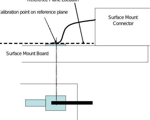
There are two major topics that together comprise the IUT identification: reference ‘plane’ definition and physical IUT boundary description.

(30)

The IUT’s of interest for this document typically have separable connectors on both ends of the IUT. Following the paradigm in SFF-8410, the IUT nominally begins and ends on the test fixture

at the point where connector joins the substrate. Part of the IUT intrinsically involves connector halves that are not part of the separable IUT as shown in

A B

C D

TP1

PHYSICAL INTERCONNECT

TP2

UNDER TEST