Draft Technical Support Document: In-Use Testing for Heavy-Duty Diesel Engines and Vehicles

(1)

Office of Transportation and Air Quality

EPA420-D-04-003 June 2004

Draft Technical Support

Document: In-Use Testing for

Heavy-Duty Diesel Engines and

Vehicles

(2)

EPA420-D-04-003 June 2004

Draft Technical Support Document:

In-Use Testing for Heavy-Duty Diesel

Engines and Vehicles

Assessment and Standards Division Office of Transportation and Air Quality

U.S. Environmental Protection Agency

NOTICE

This Technical Report does not necessarily represent final EPA decisions or positions. It is intended to present technical analysis of issues using data that are currently available.

The purpose in the release of such reports is to facilitate an exchange of technical information and to inform the public of technical developments.

(3)

CHAPTER 1

Economic Assessment

This chapter contains our economic analysis of the potential costs associated with the proposal to implement a manufacturer-run, in-use NTE testing program for heavy-duty diesel engines and vehicles. The eventual cost of the program is dependent on several key variables. One of these is the number of vehicles tested under the Phase 1 and 2 testing schemes. This, of course, depends on how many vehicles pass, or fail, the vehicle pass criteria at various points under the tiered testing procedures. Also important is just how each manufacturer will chose to design and conduct the test program, how many portable emission measurement systems

(PEMS) will be purchased, and the availability of test vehicles. Obviously, it is difficult to project these variables for an all new program. However, based on our experience with in-use emissions testing, including the development and use of a portable emission measurement device for compliance testing, we have identified a set of reasonable testing scenarios that allow us to estimate the potential costs associated with the proposed program.

This chapter is divided into several parts. Section 1.1 contains a brief outline of the

methodology used to estimate the associated costs is presented. Section 1.2 develops the fixed and variable cost components associated with the program. Section 1.3 summarizes the component costs into estimates of the overall cost of the program. All costs are estimated in 2003 dollars.

1.1 Overview

All costs are divided into either fixed or variable cost components. Fixed costs are associated with the direct expense of purchasing the requisite portable emission measurement system (PEMS) units. Variable costs depend primarily on the number of families and vehicles tested. They include the direct costs for vehicle recruiting, labor for on-site testing, instrument calibration and maintenance, travel, data analysis, and reporting expenses. Variable costs also include indirect costs associated with overhead and general and administrative (G&A) expenses.

To explore the range of possible costs, we developed two testing scenarios that differ in the relative availability of test vehicles (i.e., how difficult it is to access, instrument, and test vehicles at a job site), and the type and amount of travel required to conduct the test campaign (e.g., overnight versus local travel). We also assessed a range of costs associated with different testing intensities under Phase 1 or Phase 2 of the program (i.e., the amount or number of vehicle tests that might occur under the two phases of testing). Finally, we combined this information to show a range of possible costs and a single point estimate by assuming a specific mix of the above testing variables. The results are presented for all heavy-duty engine manufacturers as annualized costs, total costs for the first five years of the program, and costs over 30 years.

(6)

1.2 Cost Components 1.2.1 Fixed Costs

Fixed costs for this program are primarily associated with buying PEMS units. Some of the fixed cost components have significant uncertainties associated with them. Portable

measurement devices are already commercially available that can measure all the gaseous pollutants required by the proposed program. These systems cost approximately $70,000 per unit. Based on our experience and investment in developing portable particulate matter (PM) measurement technology, we estimate that systems capable of measuring both gaseous and PM emissions will cost an additional $30,000 per unit.1_{Therefore, the capital cost for portable} measurement devices that measure both gaseous and PM emissions is approximately $100,000 per unit.

As described in Chapter 2 of this document, we assume that engine manufacturers will initially purchase PEMS units with the capability to measure gaseous pollutants in time to coincide with the initiation of the pilot program at the start of the 2005 calendar year. Add-on, modular devices that measure PM emissions will be purchased later in 2005 as this technology becomes available. Regardless of the purchasing strategy, we assume all equipment purchases occur at the beginning of 2005 in order to simplify the analysis.

We estimate that portable emission measurement devices have a product life cycle of five years for the purposes of the proposed program. After that time they are assumed to be replaced with brand new equipment. Also, we assume there is no salvage value for units that may remain in service for other less rigorous or less important duties after five years, although this could occur in some instances. Alternatively, some manufacturers may chose to replace or rebuild component parts of a PEMS unit rather than replace the entire unit after five years. To the extent this may occur, we assume such a maintenance strategy will cost approximately the same as the replacement strategy. The annualized cost of a single PEMS unit can now be calculated by using the above values and assuming a typical capital recovery rate of seven percent per annum. The result is an annualized cost of $24,390 per unit.

The total annualized fixed cost for the program depends on how many PEMS units each manufacturer will purchase, the fraction of time the equipment is used for the in-use testing program, and the number of manufacturers subject to the requirements. Each of these cost components is addressed separately below.

We assume that each manufacturer will purchase two units. We chose this number to illustrate the average equipment cost of the program recognizing that two units is adequate to perform more than the needed amount of tests for even the largest manufacturer if its program is

1_{Chapter 2 contains additional information on the status and development of portable} emission measurement systems.

(7)

designed so that testing can be conducted in an orderly, efficient manner. We recognize that manufacturers with a limited number of engine families may need only one unit. Conversely, manufacturers with a large number of families may prefer additional units. However, we think that two units is adequate for the average manufacturer.

We also expect that manufacturers will likely want a spare unit in the field beyond the two PEMS that may be in service, to prevent disrupting the test program if a serious, unserviceable problem arises with one of the primary systems. We expect that the spare unit will be taken from other PEMS units the manufacturer has purchased for separate engine or emission control

technology development work. Rather than trying to estimate the cost of such a practice, we are making an offsetting assumption that the PEMS units purchased for the proposed in-use testing program are also sometimes used for other purposes, e.g., engine and emission control

technology development. We anticipate that these units would otherwise often be idle, because the intensity of the test requirements associated with the in-use testing program will result in significant periods of downtime for these units.

Our final assumption in estimating the total annual fixed cost of the proposed program is that 14 engine manufacturers will participate in the program. This is the number of companies that certified heavy-duty diesel engines in the 2003 model year. The manufacturers are shown below.

Caterpillar, Inc.

Cummins Engine Company, Inc. DaimlerChrysler AG

Detroit Diesel Corporation General Engine Products General Motos Corporation Hino Motors, Ltd.

International Truck and Engine Corporation Isuzu Motors Limited

Mack

Mitsubishi Motors Corporation Nissan Diesel Motor Co., Ltd. Scania CV AB

Volvo Powertrain Corporation

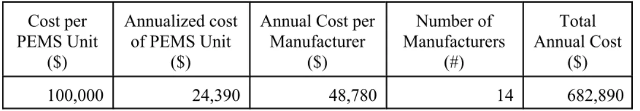
Using the above information, the total annualized fixed cost of the proposed program $682,890, as shown in Table 1-1.

1.2.2 Variable Costs

Variable costs are grouped into two broad categories: cost per vehicle test and cost per family. This approach allows us to more easily account for tests that must be repeated on the same vehicle in order to obtain a valid test result. Repeat testing can occur in the laboratory due

(8)

to equipment or vehicle malfunctions, and operator error. We expect that similar problems may occur in field testing, and assume that these issues can generally be remedied at the testing location. Further, a vehicle may be tested a second day under the terms of the proposed program if less than three hours of non-idle operation are recorded during the first “shift day” of testing. Obviously, multiple tests on the same vehicle do not directly affect other costs associated with testing an engine family, e.g., vehicle recruiting. Therefore, these costs are estimated separately in our analysis.

Also, as noted earlier, many of the costs of the proposed program vary by the relative

availability of test vehicles (i.e., how difficult it is to access, instrument, and test vehicles at a job site), and the type and amount of travel required to conduct the test campaign (e.g., overnight versus local travel). In order to reasonably bracket these cost elements, we constructed two testing scenarios that differ in the above characteristics. These scenarios are based on our direct experience in conducting in-use testing of heavy-duty trucks with portable emission

measurement systems under the 1998 consent decrees, our continued development of portable measurement systems, and a recently awarded EPA contract to conduct a large scale, in-use testing pilot program in Kansas City, Missouri for passenger cars (USEPA 2003). The two testing scenarios are described in the following section by first identifying some of the key elements shared by both scenarios and then presenting the specifics of each scenario separately.

1.2.2.1 General Description of Testing Scenarios

Our testing scenarios share a number of key assumptions which we believe provide a reasonable representation of how manufacturers are likely to design and conduct testing under the proposed program. Alternatively, if an engine manufacturer decides to contract for testing services, we expect the service provider to similarly design and conduct the testing campaign.

One of our most basic methodological assumptions is that field testing will usually consist of a multi-day campaign where a minimum of five vehicles are tested. This number was chosen for several reasons. First, it captures the type of back–to-back vehicle testing likely to be employed in order to facilitate efficient testing. Second, it represents the minimum number of test vehicles for Phase 1 testing under the proposed program. Third, and finally, it simplifies the analysis when evaluating the potential costs of higher testing intensities associated with the maximum number of vehicles that may be tested under Phase 1 (10 total vehicles) and Phase 2 (20 total vehicles). These later testing levels are simple multiples the Phase 1 minimum testing scenario, i.e., two times or four times, respectively. Other key assumptions are described below.

S Vehicle recruiting and pre-screening of prospective test vehicles will be done by telephone or other means prior to the test site visit.

S All portable measurement systems will be inspected and pre-calibrated at the manufacturer’s facility prior to deployment in the field.

S Field testing will be conducted by two people. One is an engineer and the other a qualified technician. Both are capable of installing and operating the portable measurement systems, screening vehicles for OBD trouble codes and MIL

(9)

also capable of performing all required inspections of the vehicle’s mechanical, electrical, and emission control systems; as well as performing allowable maintenance and the setting of adjustable engine parameters as required.

S The test engineer and technician will coordinate their activities to optimize their productivity. For example, the engineer may acquire and enter a vehicle’s history and vital statistics into an electronic database concurrently while the technician performs vehicle inspection and allowable maintenance.

S Test vehicles for an engine family are obtained from two independent sources, as required by the proposed regulation. It is assumed that the sources are located relatively close to each other to minimize travel distances between test sites.

S The test sites will be in relatively close proximity to a manufacturer’s technical center, test center, maintenance facility, or other similar location to minimize personnel travel and field logistics.

S Test vehicles will depart and return to the same location the same day. Further, a “shift day” is approximately eight hours in duration.

S Field personnel have access to the test vehicles and a service location before and after the shift day as needed to install and remove the portable measurement devices. Special arrangements with the vehicle owner/operator may be necessary.

S Two portable emission measurement systems will be deployed simultaneously during a test site visit when possible, i.e., two vehicles will be tested at the same time.

S All necessary tools, spare parts, testing supplies, office supplies, etc. will be taken to or otherwise supplied at the site of testing to avoid unnecessary delays.

One of the key simplifying assumptions from above is that the test vehicles will be away from their home base for a single day. It is also possible that test vehicles may be operated on multi-day driving routes, i.e., long-haul operation. We do not think this will be a standard practice, but may happen from time to time. To the extent it does occur, the cost of such tests may be somewhat higher than reflected in this analysis. For example, the field logistics and site visits may be more complex. Also, even though a PEMS unit is capable of operating unattended for extended times, it may require a suitably sized gas bottle for the Flame Ionization Detector (FID), which would increase the cost of the test. We believe it is unlikely that the PEMS unit would need to be calibrated or otherwise maintained by a technician during a multi-day test, although this has not been demonstrated in actual field testing. Finally, in the event that fuel or self-contained standby battery power is expended, the unit will simply shut itself off. We assume that upon returning home, the system would checked, calibrated, and the emissions data downloaded as described next.

Each of the test scenarios also share some of the same core on-site work activities. These categories are described below in their approximate order of occurrence.

S Vehicle History/Documentation. Obtaining all relevant information not available prior to the field visit or verifying the accuracy of information previously obtained.

S Vehicle Set-to-Specification. Inspecting the vehicle, performing allowable maintenance, and setting all adjustable engine control parameters.

(10)

S PEMS Installation. Install the portable measurement system onboard the test vehicle. Warm the instrument to operating temperature, verify proper operation, perform final calibrations and span instruments, etc.

S PEMS Data Acquisition. Download the measurement data set; perform on-site data verification and initial quality assurance; and record and store all other relevant test information.

S PEMS Removal. Verify proper operation, perform post-test calibration, and remove system from the test vehicle.

S Miscellaneous Time. Non-routine labor for repairing or replacing parts of the

portable emission measurement systems or test vehicles, obtaining supplies not at the test site, etc.

Now that the overall components of the testing scenarios have been identified, the specific scenarios will be presented.

Scenario 1 –Easy Vehicle Access and Local Travel

In this scenario the owner/operator of the test vehicles make them readily available on an “as needed” basis so that the testing personnel can execute the test program in an expeditious

manner. This means, for example, there will be little or no “idle” time while at the job site waiting for a vehicle to become available for either installing or removing the portable

measurement system. Also, the test sites are located close enough to the manufacturer’s facility, or employees base of operation, so they can commute to and from the job each day. This avoids overnight travel expenses. This scenario reflects how most of EPA’s in-use testing is conducted under the consent decrees.

Scenario 2 – Limited Vehicle Access and Overnight Travel

This scenario reflects a less time efficient case than Scenario 1. Test vehicles are not readily available and the testing technician and engineer must sometimes work around a test vehicle’s normal daily work shift. This means that the work day for the testing personnel includes the time the vehicle is being driven over its normal work route. In these instances, we made a worst case assumption that the testing personnel remain “idle” on the job site, with this time charged to the in-use testing program. In reality, we expect that the engineer and technician may perform work that could be billed to other assignments for all or part of this time. Also, the test sites are located far enough away from the manufacturer’s facility, or employees home base, that a single round trip to and from the job site and overnight travel is required. However, the sites are still close enough to one another that travel between the two locations is not restrictive or prohibitive.

(11)

1.2.2.2 Variable Cost Per Test

As described above, the cost to perform an individual vehicle test is based on a Phase 1 testing scheme where a minimum of five vehicles must be tested. Test costs consist of direct labor, labor overhead, other direct costs, and general and administrative overhead. Each of these cost components is described below.

1.2.2.2.1 Direct Labor

The cost of direct labor for each scenario is estimated by applying an hourly compensation rate by labor category to the various activities associated with the field testing campaign. Tables 1-2 and 1-3 display the work flow for Scenario 1 and 2, respectively, broken down by activity, labor type, and number of hours spent preforming each activity. These depictions reflect the assumptions, work activities, and optimization of the work flow as described in Section 1.2.2.1. The time spent in the various work tasks are estimated based on EPA’s direct experience in conducting in-use testing with portable emission measurement devices and on the recently awarded Kansas City, Missouri test program.

The test campaign for Scenario 1 is completed in four days. It is assumed that the testing personnel return to the manufacturer’s facility at the end of Day 4 for to work on other

assignments. The total direct labor is 27 hours for the engineer and 27 hours for the technician. Scenario 2 is completed in five days. The lack of vehicle flexibility leads to long work days in this scenario. The total direct labor is 55 and 56 hours for the engineer and technician,

respectively.

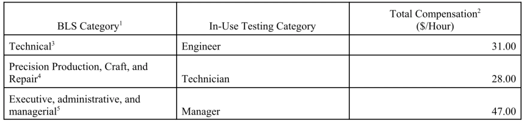
We developed an hourly estimate of employee compensation from information published by the Bureau of Labor Statistics, Office of Compensation and Working Conditions, Employer Costs for Employee Compensation (BLS 2003). Table 1-4 shows our estimate of $31 and $28 per hour for an engineer and technician, respectively. These hourly compensation rates are “total compensation,” and include wages and salaries, paid leave, supplemental pay, and insurance. By comparison, these labor rates compare well with the contract labor costs we incur in conducting our in-use testing under the consent decrees. Finally, we assume that labor exceeding 40 hours per week is paid as overtime, i.e., 1.5 times the normal hourly rate.

For convenience, Table 1-4 also shows an hourly compensation rate for a manager using the same literature source as described above. This labor category will be used in Section 1.2.2.3, where variable costs are discussed.

The resulting direct labor cost per test can now be calculated based on the above labor hours and hourly compensation rates. As shown in Table 1-5, the resulting per test cost is $319 and $757 for Scenario 1 and 2, respectively.

(12)

1.2.2.2.2 Labor Overhead

We assume that all direct labor is burdened at 100 percent of the total compensation rate. For simplicity, overtime pay is also burdened at this same overhead rate.

1.2.2.2.3 Other Direct Costs

A number of other costs not related to labor that are “consumed” during in-use testing include office supplies such as office supplies, DVDs, calibration gases, and fuel for the flame ionization detector (FID). Based on our experience with using portable measurement systems, we estimate that calibration gases will cost about $75 per test and all other supplies will cost about $25 per test. Therefore, we estimate that a total of $100 per test for other direct costs.

1.2.2.2.4 Repeat Tests

Some in-use tests will be voided due to operator error and test equipment malfunctions. Other tests will be repeated if less than three hours of non-idle vehicle operation are recorded during the first day of testing. At our National Vehicle Fuel and Emissions Laboratory in Ann Arbor, Michigan, we experienced a test void rate for laboratory-based, non-research testing of approximately four percent over the last two years. We expect a somewhat higher void rate for field testing. Also, as noted, some tests will be repeated do to the three hour non-idle

requirement. Overall, we assume a combined repeat test rate of 10 percent for this analysis. 1.2.2.2.5 General and Administrative Overhead

Certain costs are incurred for common or joint objectives and therefore cannot be identified specifically with a particular project or activity. We assume these general and administrative costs to be 6.5 percent of all other costs.

1.2.2.2.6 Summary of Variable Cost per Test

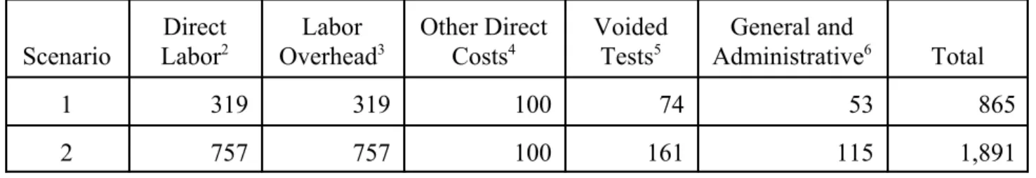
Table 1-6 summaries the various direct cost elements described above. As shown, the resulting total variable costs per test are $865 and $1,891 for Scenario 1 and 2, respectively.

1.2.2.3 Variable Cost Per Engine Family

As with the previous section, the cost per engine family is based on a Phase 1 testing scheme where a minimum of five vehicles must be tested. This overall cost is composed of a number of individual expenses such as paying the test vehicle’s owner/operator an incentive, recruitment, travel, instrument pre-calibration, data analysis, and reporting. Each of the cost elements are described below.

(13)

1.2.2.3.1 Vehicle Incentives

We generally offer a vehicle’s owner an incentive in the form of a government bond and free vehicle repairs as part of our in-use test programs. Sometimes the owner cooperates without such an incentive, as most often occurs in our in-use testing under the consent decrees. For the purposes of this analysis, we assume that a cash incentive of $150 per vehicle will be paid to the owner by the engine manufacturer. This is the average cost of the incentive, with some owners being offered more some less, and some cooperating without an incentive. Therefore, the total incentive for an engine family tested under the Phase 1 minimum requirements is $750.

1.2.2.3.2 Direct Labor

Each engine family will incur costs in three principle labor categories: vehicle recruitment, instrument pre-calibration, and data analysis and reporting. We expect that manufacturers will rely heavily on their existing customer relationships to recruit appropriate test vehicles from fleets or individual owners. Alternatively, they will create new lines of communication with their customers. A significant amount of pre-screening and vehicle history will also be associated with vehicle recruitment. We assume that with a heavy emphasis on existing customer relationships and data bases, recruiting the requisite five test vehicles will average about $300 per engine family.

Prior to being deployed in the field, each portable measurement system will be carefully examined at the manufacturer’s facility to ensure proper operation. Based on our experience with portable emission measurement systems, we estimate that pre-calibrating each unit will require 0.5 and 1.5 hours of engineer and technician time, respectively. Using the total compensation rates previously described in Table1-4, this would cost $58 per unit. Since it is assumed that testing will be conducted using two portable systems, the total direct labor cost for pre-calibrating the instruments is $116 per engine family.

The last category of direct labor per engine family is primarily for final data analysis and quality assurance (beyond that which is conducted in the field), reporting results, and archiving information. We assume that engine manufacturers will develop a number of automated methods to perform many of these functions to minimize labor requirements. Our direct labor estimates are basically taken from another EPA report that was prepared to support a new pilot program aimed at developing new in-use data collection methods for nonroad diesel-powered equipment (USEPA 2004). That program will also collect, analyze, and report emissions data using portable emission measurement systems. For the purposes of this analysis, we doubled the time per test for managerial oversight, since the original estimate was developed to reflect an emission factor style program, while the proposed in-use program has more important

compliance implications.

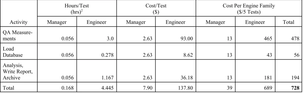
Table 1-7 presents the estimated labor hours for each data analysis and reporting activity, the cost per test, and the cost per engine family. The cost per test is based on a labor rate of $31 per hour for an engineer and $47 per hour for a manager. These labor classifications and

(14)

compensation rates were previously discussed in Section 1.2.2.2 and presented in Table 1-4. The total cost of post-data analysis and reporting is estimated to be $728 per engine family.

The resulting total direct labor for the three categories described above is $1,144 per engine family.

1.2.2.3.3 Travel

Our basic assumptions regarding travel needs are described in Section 1.2.2.1. The costs of travel are divided into direct labor, vehicle costs, and per diem expenses for room and board. For Scenario 1, we assume the test sites are located close enough to the manufacturer’s facility, or employees base of operation, so they can commute to and from the job site each day. This avoids overnight travel expenses. More specifically, we assume that commuting at the

beginning and end of each work day is 30 minutes each way, two trips occur per day, and there are four testing days for a total of four hours. There is also 30 minutes of travel time between test sites on Day 2 and Day 3 (Table 1-2). Based on these assumptions, the total travel time is five hours. Using the total compensation rates previously presented in Table 1-4 of $31 and $28 per hour for an engineer and technician, respectively, the travel-related direct labor cost is$236 for daily commuting and $59 for inter-site travel, or a total of $295 per engine family.

The vehicle expenses associated with Scenario 1 are estimated by using an assumed average speed of 50 miles per hour and a mileage fee of $0.40 per mile. The mileage cost is based on a federal government reimbursement rate for privately-owned vehicles of $0.365 per mile in 2003, with an increase of approximately 10 percent to account for the use of a large van or small truck. We assume such a vehicle will be required to transport the portable systems and supplies, and provide a small work space if needed. Using the commuting time of 4 hours, 50 miles per hours, and $0.40 per mile the total travel related vehicle cost is $80 per engine family. Combining this with the travel-related labor of $295, the total travel cost for Scenario 1 is $375 per engine family.

For Scenario 2, we assume the test sites are located far enough away from the manufacturer’s facility, or employees home base, that a single round trip to and from the job site and overnight travel is required. More specifically, we assume that commuting at the beginning and end of the work week is four hours one way for a total of eight hours. Again, using the total compensation rates previously presented in Table 1-4 of $31 and $28 per hour for an engineer and technician, respectively, the travel-related direct labor cost is $472 per engine family.

The vehicle expenses associated with Scenario 2 consist of the round trip travel to the testing locations described above, and daily travel to and from the test sites as well as itinerant travel, e.g., lunch and dinner. The round trip travel expense associated with the eight hours of commuting time is estimated by using an assumed average speed of 50 miles per hour and a mileage fee of $0.40 per mile. The result is $160. The itinerant travel distances are assumed to be 30 miles for Day 1 and 45 miles each day for the next three days, or a total of 165 miles. Using the assumed vehicle reimbursement fee, this amounts to $66.

(15)

This scenario requires overnight travel. There will be approximately four days of full per diem expenses and a partial day of meals on the fifth day (Table 1-3). We assume it costs $100 per night for lodging and $40 per day for meals. This results in per diem expenses of $600 for the full week. Combining this with the travel-related labor of $472 and the vehicle cost of $66 from above, the total travel cost for Scenario 2 is $1,138 per engine family.

1.2.2.3.4 Labor Overhead

We assume that all direct labor is burdened at 100 percent of the total compensation rate. 1.2.2.3.5 General and Administrative Overhead

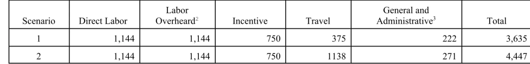
We assume general and administrative expenses to be 6.5 percent of all other costs. 1.2.2.3.6 Summary of Variable Cost per Engine Family

Table 1-8 summaries the various cost elements discussed above. As shown, the resulting total variable costs per engine family are $3,635 and $4,447 for Scenario 1 and 2, respectively. 1.3 Costs of the Proposed Program

Now that the basic fixed and variable cost inputs for each of the two scenarios have been developed, we will use that information to identify a range of total annual costs for the proposed program. This range reflects the two testing scenarios, as described in Section 1.2.2.1, and three different levels of testing intensity that may occur under the Phase 1 and 2 requirements, which are described below. We will also develop a single point estimate of the proposed program’s annual cost. Finally, we will use this point estimate to present total costs for the first five years of the program, and costs over 30 years. These costs are presented for the entire industry.

The first level of testing intensity is the minimum number of vehicles that must be tested under Phase 1 of the proposed program to demonstrate if a designated engine family passes the NTE criteria, i.e., five vehicle tests per family. This is the basis upon which the variable cost components were developed in Section 2.1, and is referred to as Phase 1 minimum. The second level of testing is the maximum number of vehicles that could be required under Phase 1, i.e., 10 vehicle tests per family. This is referred to as Phase 1 maximum. The third level of testing is a worst case where a manufacturer must complete Phase 2 testing for an engine family. At its maximum, Phase 2 requires up to 20 vehicle tests per family. This is referred to as Phase 2 maximum.

Overall, our methodology for estimating the costs associated with the three testing levels is simple. We assume that a manufacturer will complete each level of testing in discreet steps. For example, after completing Phase 1 minimum, the test results for the engine family will be

thoroughly evaluated at the manufacturer’s technical center. If one or more of the vehicles do not pass the testing criteria, the manufacturer is assumed to return to the field to continue testing

(16)

five more vehicles, i.e., Phase 1 maximum. For the purposes of this analysis, this means that the variable cost of Phase 1 maximum testing is twice the cost of performing Phase 1 minimum testing. Similarly, the variable cost of Phase 2 maximum, i.e., 20 vehicles, is twice the cost of Phase 1 maximum, i.e., 10 vehicles. The fixed cost of testing is constant for each of the three testing intensities, since the cost of purchasing the portable measurement systems does not change with the number of tests performed.

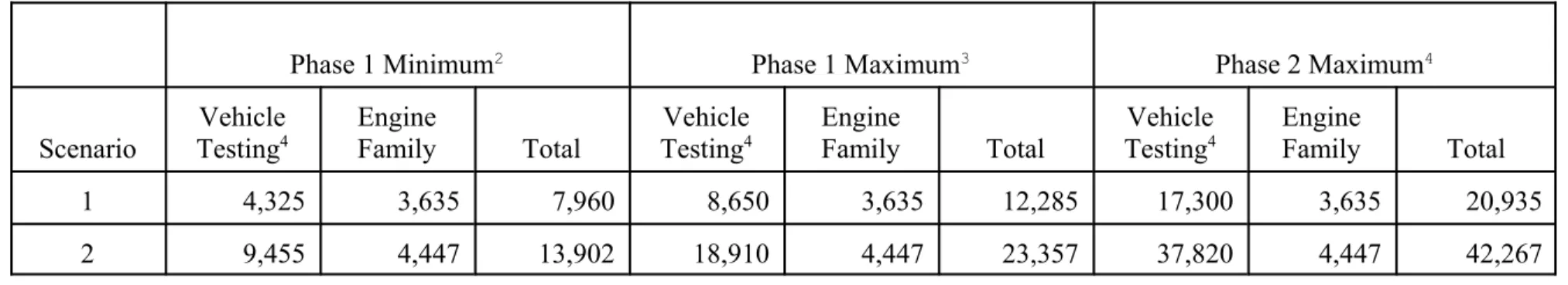
1.3.1 Variable Costs by Level of Testing Intensity

As noted above, fixed costs do not change by the number of tests performed, although variable costs do vary by testing intensity. Therefore, the first step in estimating the range of annual costs is to determine variable cost per family for each of the testing levels. This is presented in Table 1-9 for the two test scenarios.

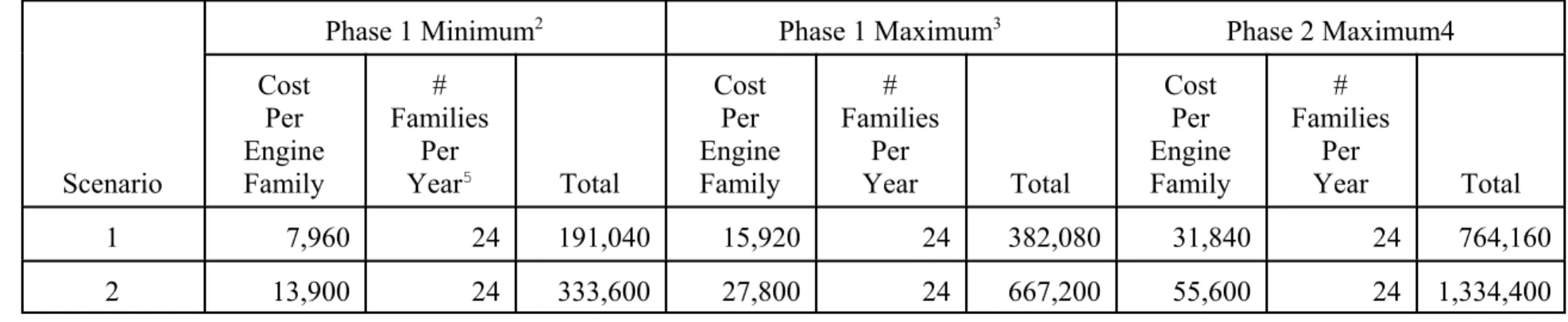
The next step is to find the range of annual costs for all manufacturers, i.e., all engine families. Under the proposed program, we may generally select up to 25 percent of an engine manufacturer’ families for testing each year. In the 2003 model year, there were 95 heavy-duty diesel engine families certified. Hence, we may select up to 24 engine families per year. Using this value, the resulting range of annual costs for all manufacturers is shown in Table 1-10.

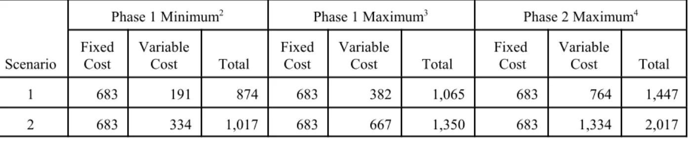
1.3.2 Total Annual Costs by Level of Testing Intensity

Table 1-11 summarizes the fixed and variable cost estimates and presents the total annual cost for each test scenario and testing level. The low end of the range is about $874 thousand per year for Phase 1 minimum, and the high end of the range is $2.02 million for Phase 2 maximum.

1.3.3. Total Annual Cost Point Estimate

Our point estimate assumes the overall program will reflect the average of the two scenarios and weighted at 90 percent of the Phase 1 minimum average cost and 10 percent of the Phase 2 maximum average cost. This reflects our belief that most of the engine families will be designed and built in full conformance with the applicable NTE standards. But also that the program will identify some level of potential nonconformance. Table 1-12 summarizes the Phase 1 minimum and Phase 2 maximum costs from the previous table for convenience and presents our point estimate of the total annual cost for all manufacturers. The point estimate is $1.02 million per year.

(17)

1.3.4. Total Costs Over 5 and 30 Years

We developed an estimate of the total program costs over both 5 and 30 years using the annual point estimate costs from Table 1-13 and a discount rate of seven percent per annum. As shown, the 5 year cost is about $7.82 million and the 30 year cost is about $33.5 million.

(18)

Chapter 1 References

1. U.S. Environmental Protection Agency. 2003. Characterizing Exhaust Emissions from Light-Duty Gasoline Vehicles in the Kansas City Metropolitan Area. ERG. EPA Contract Number GS-10F-0036K. Office of Transportation and Air Quality, Assessment and Standards Division, Ann Arbor, Michigan. Awarded February 2004.

2. Bureau of Labor Statistics. 2003. Employer Costs for Employee Compensation-June 2003.

USDL: 03-446. U.S. Department of Labor, Washington, D.C.

3. U.S. Environmental Protection Agency. 2004. Mobile Source Emission Factors:

Populations, Usage and Emissions of Diesel Nonroad Equipment in EPA Region 7. Agency Form Number 0619.11, Supporting Statement, Part A. Office of Transportation and Air Quality. March 2004. EPA Edocket No. OAR-2003-0225-0003.

(19)

Table 1-1. Total Annualized Fixed Costs1 Cost per PEMS Unit ($) Annualized cost of PEMS Unit ($)

Annual Cost per Manufacturer ($) Number of Manufacturers (#) Total Annual Cost ($) 100,000 24,390 48,780 14 682,890 1_{2003 dollars.}

(20)

Table 1-2. Scenario 1 – Easy Vehicle Access and Local Travel

Day 1 Day 2 Day 3 Day 4 Day 5

Activity Hrs Labor Type Activity Hrs. Labor Type Activity Hrs Labor Type Activity Hrs Labor Type Activity Hrs Labor Type Travel

(Location 1) 0.5 B1 Travel _{(Location 1)} _0.5 _B _{(Location 1)}Travel _0.5 _B Travel _{(Location 2)} _0.5 _B Not _Applicable

V1, V22

History 2 E V1, V2 Data Acquisition 1 B V3 Data Acquisition 0.5 B V4,V5 Data Acquisition 1 B V1, V2

Set-to-Spec 2 T V1, V2 Remove 1.5 B V3 Remove .75 B V4, V5 Remove 1.5 B V1, V2

Install

Warm 3 B V3 History 1 E Travel (Location 2) 0.5 B Misc. Time .25 B Misc. Time 1 B V3 Set-to-Spec 1 T V4, V5 History 2 E Travel (Home) 0.5 B Travel (Home) 0.5 B V3 Install Warm 1.5 B V4, V5 Set-to-Spec 2 T Misc. Time 1 B V4, V5 Install Warm 3 B Travel

(Home) 0.5 B Misc. Time 1 B Travel

(Home) 0.5 B

Totals 7 T 7 T 9 T 4 T

7 E 7 E 9 E 4 E

1_{T=Technician, E=Engineer, B=Both.} 2_{V = Vehicle (identifier).}

(21)

Table 1-3. Scenario 2 – Limited Vehicle Access and Overnight Travel

Day 1 Day 2 Day 3 Day 4 Day 5

Activity Hrs Labor Type Activity Hrs Labor Type Activity Hrs Labor Type Activity Hrs Labor Type Activity Hrs Labor Type Travel 4 B1 V1, V2 _Warm-Up ₁ _T _SpecV4 Set-to- ₁ _T V5 Set-to-_Spec ₁ _{T Travel} ₄ _B

V1, V22

History 2 E Shift Wait Time 8 B V4 History 1 E V 5 History 1 E V1, V2

Set-to-Spec 2 T V3 Set-to-Spec 1 T V4 Install V3 Warm 1.5 B V5 Install 1.5 B V1, V2 Install 3 B V3 History 1 E Shift Wait Time 8 B Shift Wait Time 8 B

Misc. Time 1 B V1, V2 Data Acquisition 1 B V3, V4 Data Acquisition 1 B V5 Remove .75 B V1, V2

Remove 1.5 B V3, V4 Remove 1.5 B V5 Data Acquisition .5 B V3 Install 1.5 B Misc. Time 1 B Misc. Time 1 B Misc. Time 1 B

Totals 10 T 15 T 14 T 13 T 4 T

10 E 14 E 14 E 13 E 4 E

1_{T=Technician, E=Engineer, B=Both} 2 _{V = Vehicle (identifier).}

(22)

Table 1-4. Labor Compensation Rates

BLS Category1 _{In-Use Testing Category} Total Compensation

2

($/Hour)

Technical3 _Engineer _31.00

Precision Production, Craft, and

Repair4 _Technician _28.00

Executive, administrative, and

managerial5 _Manager _47.00

1_{BLS 2003.}

2_{Total compensation includes wages and salaries, paid leave, supplemental pay, and insurance. Rounded to the nearest whole dollar. June}

2003 dollars.

3_{Table 11, Private industry, goods-producing and service-producing industries, by occupational group; All workers, goods-producing}

industries; White-collar occupations; Professional specialty and technical.

industries; Blue-collar occupations; Precision production, craft, and repair.

(23)

-- -- --

--Table 1-5. Direct Labor Costs Per Vehicle Test

1

(Based on Phase 1 Minimum Five Vehicle Tests per Engine Family)2

Scenario

Labor Rate Type

Hours Per Family (5 tests)

Hourly Compensation ($ per hour) Total Cost ($/5 tests) Cost Per Test ($/test)

Engineer Technician Engineer Technician

1 Regular 27 27 31 28 1593 319

2 Regular 40 40 31 28 2360 472

Overtime2 ₁₅ ₁₆ ₄₆ ₄₆ ₁₄₂₆ ₂₈₅

S2 Total 3786 757

1_{June 2003 dollars.}

2_{Based on Phase 1 testing five vehicles.}

(24)

1 2 3 4 5 6

Table 1-6. Variable Costs Per Test Vehicle

1

($/test)

Scenario

Direct

Labor2 _OverheadLabor 3 Other Direct _Costs4 Voided _Tests5 _{Administrative}General and 6 _Total

1 319 319 100 74 53 865

2 757 757 100 161 115 1,891

2003 dollars. See Table 1-5.

100 percent of direct labor.

General supplies, PEMS maintenance, calibration gases, FID fuel, etc.

Assumes 10 percent of tests are void (i.e., 0.10 * (direct labor, labor overhead, and other direct costs)). 6.5 percent of all costs.

(25)

Table 1-7. Post-Test Data Analysis and Reporting Variable Cost Per Family

1

Activity

Hours/Test

(hrs)2 Cost/Test _($) Cost Per Engine Family _{($/5 Tests)}

Manager Engineer Manager Engineer Manager Engineer Total

QA Measure ments 0.056 3.0 2.63 93.00 13 465 478 Load Database 0.056 0.278 2.63 8.62 13 43 56 Analysis, Write Report, Archive 0.056 1.167 2.63 36.18 13 181 194 Total 0.168 4.445 7.90 137.80 39 689 728 1_{2003 dollars.} 2_{See USEPA 2004.}

(26)

Table 1-8. Summary of Variable Costs Per Engine Family

1

($/family)

Scenario Direct Labor OverheardLabor 2 _Incentive _Travel

General and Administrative3 _Total 1 1,144 1,144 750 375 222 3,635 2 1,144 1,144 750 1138 271 4,447 1_{2003 dollars.} 2 _{100% of direct labor.} 3_{6.5% of all costs.}

(27)

Table 1-9. Summary of Variable Costs Per Engine Family by Level of Testing Intensity

1

($)

Phase 1 Minimum2 _{Phase 1 Maximum}3 _{Phase 2 Maximum}4

Scenario

Vehicle

Testing4 Engine _Family _Total _TestingVehicle 4 Engine _Family _Total _TestingVehicle 4 Engine _Family _Total

1 4,325 3,635 7,960 8,650 3,635 12,285 17,300 3,635 20,935

2 9,455 4,447 13,902 18,910 4,447 23,357 37,820 4,447 42,267

1_{2003 dollars.}

2_{Phase 1 minimum = 5 test vehicles.} 3_{Phase 1 maximum = 10 test vehicles.} 4_{Phase 2 maximum = 20 test vehicles.}

(28)

Table 1-10. Total Annual Variable Costs for All Manufacturers by Level of Testing Intensity

1

($)

Scenario

Phase 1 Minimum2 _{Phase 1 Maximum}3 _{Phase 2 Maximum4}

Cost Per Engine Family # Families Per Year5 _Total Cost Per Engine Family # Families Per Year Total Cost Per Engine Family # Families Per Year Total 1 7,960 24 191,040 15,920 24 382,080 31,840 24 764,160 2 13,900 24 333,600 27,800 24 667,200 55,600 24 1,334,400 1_{2003 dollars.}

2_{Phase 1 requires that a minimum of 5 test vehicles.} 3_{The maximum number of vehicles tested in Phase 1 is 10.} 4_{The maximum number of vehicles tested through Phase 2 is 20.} 5_{25% of a total of 95 engine families certified in the 2003 model year.}

(29)

Table 1-11. Total Annual Costs for All Manufacturers by Level of Testing

1

Intensity

($ Thousands)

Scenario

Phase 1 Minimum2 _{Phase 1 Maximum}3 _{Phase 2 Maximum}4

Fixed

Cost Variable Cost Total Fixed Cost Variable Cost Total Fixed Cost Variable Cost Total 1 683 191 874 683 382 1,065 683 764 1,447 2 683 334 1,017 683 667 1,350 683 1,334 2,017

1_{2003 dollars.}

2_{Phase 1 minimum = 5 vehicle tests.} 3 _{Phase 1 maximum = 10 vehicle tests.} 4_{Phase 2 maximum = 20 vehicle tests.}

(30)

Table 1-12. Total Annual Cost Point Estimate for All Manufacturers

1 ($ Thousands)

Phase 1 Minimum Phase 2 Maximum Point Estimate2

Scenario Fixed Cost Variable Cost Total Fixed Cost Variable Cost Total Fixed Cost Variable Cost Total 1 683 191 874 683 764 1,447 683 248 931 2 683 334 1,017 683 1,334 2,017 683 434 1,117 Average3 ₆₈₃ ₂₆₃ ₉₄₅ ₆₈₃ _1,049 _1,732 ₆₈₃ ₃₄₁ _1,024 1_{2003 dollars.}

2_{Assumes a 90/10 split between Phase 1 minimum and Phase 2 maximum, respectively.}

(31)

Table 1-13. Total Program Cost Over 5 and 30 Years

1

(Based on Point Cost Estimate) ($)

Year Annualized Fixed Costs Annual Variable Costs Total Annual Costs 2005 682,890 1,024,000 1,706,890 2006 682,890 1,024,000 1,706,890 2007 682,890 1,024,000 1,706,890 2008 682,890 1,024,000 1,706,890 2009 682,890 1,024,000 1,706,890 2010 682,890 1,024,000 1,706,890 2011 682,890 1,024,000 1,706,890 2012 682,890 1,024,000 1,706,890 2013 682,890 1,024,000 1,706,890 2014 682,890 1,024,000 1,706,890 2015 682,890 1,024,000 1,706,890 2016 682,890 1,024,000 1,706,890 2017 682,890 1,024,000 1,706,890 2018 682,890 1,024,000 1,706,890 2019 682,890 1,024,000 1,706,890 2020 682,890 1,024,000 1,706,890 2021 682,890 1,024,000 1,706,890 2022 682,890 1,024,000 1,706,890 2023 682,890 1,024,000 1,706,890 2024 682,890 1,024,000 1,706,890 2025 682,890 1,024,000 1,706,890 2026 682,890 1,024,000 1,706,890 2027 682,890 1,024,000 1,706,890 2028 682,890 1,024,000 1,706,890 2029 682,890 1,024,000 1,706,890 2030 682,890 1,024,000 1,706,890 2031 682,890 1,024,000 1,706,890 2032 682,890 1,024,000 1,706,890 2033 682,890 1,024,000 1,706,890 2034 682,890 1,024,000 1,706,890 30 Year NPV in 2004 13,384,945 20,070,852 33,455,797 1st 5 Year NPV in 2004 3,127,436 4,689,620 7,817,056 1_{2003 dollars.}

(32)

CHAPTER 2

On-Vehicle Portable Emissions Measurement Technology Review

2.1 Overview

With respect to measurement equipment, we already have equipment readily available to measure gaseous emissions on-vehicle using the test procedures proposed for this program. Additionally, we think it is possible that PM emissions measurement equipment will be available for the start of the 2005/2006 pilot program.

In setting the NTE standard we have already taken into account the variation in emissions due to varying engine operation and ambient conditions. In addition, in this proposal, we have taken into account the measurement tolerances of on-vehicle measurement systems.

Given the very active interest in portable measurement equipment by EPA, the California Air Resources Board, and the automotive industry, and given the available lead time, we believe that measurement equipment will be widely available so that this proposed program will be fully

implemented for all regulated emissions–including PM–by 2007. For the 2005-2006 pilot program, gaseous emissions measurement equipment is already available for use at the 2005-2006 gaseous emissions levels. Complete portable systems that measure PM emissions will take additional time before they are field ready. Based on the current availability of key measurement technologies and ongoing work to develop the requisite PM sampling hardware, we are confident these systems will be widely available by 2007, and that they may be available in time for use in the pilot program beginning in 2005. This section discusses these measurement technologies and summarizes research results.

2.2 Measurement Technologies

We expect that several complete systems will be available for use in the proposed in-use testing program that will be capable of performing the measurements needed to determine whether or not a vehicle passes an on-vehicle emissions test. At a minimum, any such measurement system must include individual analyzers and sensors that can quantify the following parameters:

1. Regulated emissions concentrations in exhaust: a. Oxides of nitrogen, NOx.

b. Carbon monoxide, CO (and carbon dioxide CO2). c. Non-methane hydrocarbons, NMHC.

d. Particulate mass, PM. 2. Exhaust flow rate.

3. Engine operation: a. Speed. b. Torque.

(33)

c. Coolant temperature and intake manifold temperature and pressure. 4. Ambient conditions:

a. Temperature. b. Dewpoint. c. Altitude.

In this section we describe the measurement technologies that we expect to be used to quantify these parameters. If these technologies are properly applied, we believe that they are acceptable for measuring emissions on-vehicle. Note too that we also allow for the use of alternate technologies according to §1065.10. Note that this provision is proposed to be amended as part of another proposed rulemaking that is a companion to this notice.

1. Regulated emissions concentrations in exhaust. Emissions concentrations need to be measured to determine brake-specific emissions.

a. NOx measurement technology. We typically accept NOx measured as the sum of NO and NO2 since conventional engines and aftertreatment systems do not emit significant amounts of other NOx species. NO may be measured either by a chemiluminescence detector (CLD), a

non-dispersive ultra-violet (NDUV) detector, or a zirconia oxide (ZrO2) sensor. NO2 may be converted catalytically to NO and detected by a CLD, or it may be detected directly via NDUV or ZrO2. We believe that CLDs are not likely to be used on-vehicle due to their compressed gas requirements, and they might likely be sensitive to vehicle vibration. NDUV and ZrO2, on the other hand, are already available as components of complete on-vehicle emissions measurement systems, and they already have been performing well in on-vehicle applications. For example, a recent study by the California Air Resources Board (CARB) indicated that for 27 heavy-duty diesel chassis dynamometer tests, an NDUV-based on-vehicle system reported NOx emissions within 4.6 % of the current NOx standard, as compared to laboratory measurements.(1) We are currently studying NDUV analyzer

performance with a 2002 light-heavy duty diesel (LHDD) on a chassis dynamometer. Our results so far indicate that the NDUV-based system reported NOx within 3.1 % of our laboratory, prior to a 5000-mile cross-country road test. After running the NDUV-based system for the entire road test–with no failures, the vehicle was returned to the laboratory, and the NDUV-based system reported NOx emissions within 3.9 % of our laboratory. The manufacturer of the NDUV-based system has also indicated that several engine manufacturers have evaluated their system, and their results from 11 HDDE FTP tests indicate Nox emissions were reported within 4.4 % of the current standard in engine manufacturer’s laboratories. (1) ZrO2 sensors are expected to be used on-vehicle not only for Nox emission measurements, but also for feedback control of NOx aftertreatment systems.(2) The ZrO2 sensor needed for aftertreatment control is a component originally designed and developed for gasoline powered vehicles (in this case lean-burn gasoline vehicles) that are already well developed and can be applied with confidence in long life for NOx adsorber based diesel emission control. The ZrO2 sensor is an evolutionary technology based largely on the current Oxygen (O2) sensor technology developed for gasoline three-way catalyst based systems. Oxygen sensors have proven to be extremely reliable and long lived in passenger car applications, which see significantly higher temperatures than would normally be encountered on a diesel engine. Diesel engines do have one characteristic that makes the application of ZrO2 sensors more difficult. Soot

(34)

in diesel exhaust can cause fouling of the ZrO2 sensor damaging its performance. However this issue can be addressed through the application of a catalyzed diesel particulate filter (CDPF) in front of the sensor. The CDPF then provides a protection for the sensor from PM while not hindering its operation. Since we expect NOx measurement only downstream of a CDPF in each of the potential technology scenarios we have considered, this solution to the issue of PM sooting is already

addressed.

b. CO (and CO2) measurement technology. Since we first regulated CO, non-dispersive infra-red (NDIR) detector technology has been used for measuring CO and CO2 in laboratory applications. Many laboratory NDIR analyzers have a moving part called a chopper-wheel to pulse infra-red light through the exhaust gas sample. The pulsing light is used to alternately detect the CO and CO2 concentrations and then the dark-current of the NDIR detector. This is done to maintain accuracy, but the moving chopper-wheel is not durable under the high vibration environment of on-vehicle testing. However, new NDIR analyzers have been commercialized that electrically switch the infra red light source on and off. These new NDIR analyzers are already available in complete on-vehicle emissions measurement systems, and they have been performing well in on-on-vehicle

applications. For example, a recent study by the California Air Resources Board (CARB) indicated that for 27 heavy-duty diesel chassis dynamometer tests, an NDIR-based on-vehicle system reported CO emissions within 0.7 % of the current CO standard (2.1 % for CO2), as compared to laboratory measurements.(1) We are currently studying NDIR analyzer performance with a 2002 light-heavy duty diesel (LHDD) on a chassis dynamometer. Our results so far indicate that the NDIR-based system reported CO within 1.0 % of our laboratory (1.1 % for CO2), prior to a 5000-mile cross-country road test. After running the NDIR-based system for the entire road test–with no failures, the vehicle was returned to the laboratory, and the NDIR-based system reported CO emissions within 7.1 % of our laboratory (2.2 % of the current CO standard) and 4.7 % for CO2. The manufacturer of the NDIR-based system has also indicated that several engine manufacturers have evaluated their system, and their results from 11 HDDE FTP tests indicate CO emissions were reported within 0.5 % of the current standard in engine manufacturer’s laboratories (3.55 % for CO2).(1)

c. NMHC measurement technology. The flame ionization detector (FID) has been the measurement technology of choice for hydrocarbon measurements since the late 1950s. The FID has been used as a detector in liquid and gas chromatography systems for individual hydrocarbon speciation and quantification. It is used because of its response to a broad range of hydrocarbons, its inherent stability and its remarkably linear response from very high levels to very low levels of hydrocarbons. Because the FID responds to a very broad range of hydrocarbons, we chose to set our initial

hydrocarbon standard based on the FID response to the total hydrocarbons (THC) in engine exhaust. Later, by allowing for the subtraction of methane (CH4) from THC, we set non-methane

hydrocarbon (NMHC) standards based on the FID’s response to all non-methane hydrocarbons in engine exhaust. Because the FID has a range of response factors for all of the hydrocarbons that it detects, and because the mixture of hydrocarbon species in engine exhaust changes as a function of engine operation, fuel, and aftertreatment systems, the FID’s response to NMHC in engine exhaust is characteristic to hydrocarbon measurement via FID technology alone. This makes it almost impossible for other hydrocarbon detector technology to equivalently detect engine exhaust NMHC.

(35)

Fortunately, FIDs have been adapted for on-vehicle use. These new FID analyzers are already available in complete on-vehicle emissions measurement systems, and they have been performing well in on-vehicle applications. For example, a recent study by the California Air Resources Board (CARB) indicated that for 27 heavy-duty diesel chassis dynamometer tests, a FID-based on-vehicle system reported THC emissions within 2.8 % of the current NMHC standard, as compared to laboratory measurements.(1) We are currently studying FID analyzer performance with a 2002 light-heavy duty diesel (LHDD) on a chassis dynamometer. Our results so far indicate that the FID-based system reported THC within 7.8 % of our laboratory after running the FID-FID-based system for a 5000 mile road test–with no failures, (2.4 % of the current NMHC standard). The manufacturer of the FID-based system has also indicated that several engine manufacturers have evaluated their system, and their results from 11 HDDE FTP tests indicate THC emissions were reported within 1.3 % of the current NMHC standard in engine manufacturer’s laboratories.(1)

d. PM measurement technology. PM measurement has been traditionally conducted by depositing diluted exhaust PM on a sample filter and then weighing the filter in a PM measurement laboratory before and after testing to determine the net mass gain due to PM.

This technique has been applied to on-vehicle testing by one on-vehicle emissions measurement system manufacturer. This system was tested in the laboratory by the California Air Resources Board (CARB) and the results were compared to those from chassis dynamometer testing.(3) Thirty-three tests were run on two different heavy-duty trucks, and one of the trucks was equipped with a PM trap. The 33 emissions results were collected over five different test cycles for each truck. For the current-technology truck, on-average, the on-vehicle system reported PM results within 0.6 % of the current standard, which will also remain in effect during the 2005-2006 pilot program, when compared to laboratory results. For the trap-equipped truck, average, the on-vehicle system reported PM results within 38 % of the 2007 standard, when compared to the laboratory. However, because the trap-equipped truck was emitting PM at only 44 % of the 2007 standard (according to laboratory results), the 38 % error of the on-vehicle system would not have caused any false indication of a failure. Furthermore, neither the laboratory nor the on-vehicle system were equipped to sample PM according to our specifications for measuring PM from engines that meet the 2007 PM standards. These specifications were tailored to reduce variability in this type of PM measurement.

These filter-based results demonstrate that accurate on-vehicle PM measurement technology is already available for the current level of PM emissions, and it demonstrates that proportional sampling of PM on-vehicle is available today. However, we do not expect filter-based methods to be used for conducting NTE tests in the field. This is because for NTE testing, PM emissions must be quantified for several individual NTE events, which would require many filters and a means to switch these filters in an automated way. No such system is available or in development to our knowledge, and we believe that such an automated system might be cumbersome on-vehicle. We are currently evaluating more automated technologies for quantifying PM mass on-board. The underlying automated measurement technologies detect the inertia of particulate mass (PM) by

(36)

accelerating it via vibration, rather than detecting its weight due to the acceleration of Earth’s gravity. The inertial measurement technologies include the Tapered Element Oscillating

Microbalance (TEOM) and the Quartz Crystal Microbalance (QCM). Since these technologies are compact, they are suitable for on-vehicle applications. And since they impart greater acceleration upon PM versus Earth’s gravity, they are more sensitive than their laboratory microbalance cousins. They also eliminate the need to transport PM sample filters to a PM measurement laboratory for pre-and post-weighing. Researchers at West Virginia University have used a heavy-duty diesel engine to compare QCM and TEOM measurement devices, which can be purchased today, versus engine dynamometer testing in the laboratory. They showed that for seven repeats of EPA’s heavy-duty FTP, the TEOM and QCM devices can quantify PM within 5 % of a traditional microbalance at current emissions standards.(4)

Although these results demonstrate that this automated on-vehicle PM measurement devices exist today, more work is needed to demonstrate their accuracy in the lab and in the field. Further, conducting NTE tests in the field poses additional challenge . Namely, quantification of PM over sampling intervals as short as 30 seconds has yet to be demonstrated for engines certified to the current PM emission standards, or those that are expected to meet the more stringent standards beginning in 2007. At least initially, the technological challenge represented by such a short sampling interval may require sampling times beyond the minimum 30 second NTE event.

Additionally, because PM equilibration is required before and after each NTE event, the time it takes to equilibrate PM sample after an NTE event might prevent capturing all or part of the next NTE occurrence, if that subsequent event closely follows the previous one. Even if these limitations are not resolved, however, they can be accommodated in the design of the proposed in-use testing program. NTE sampling times longer than the 30 second minimum, or not capturing a portion of a valid NTE sampling event, simply means that some potential NTE samples will not be detectable. In addition to the measurement technologies described above, work is continuing to miniaturize on-board proportional sampling devices, and to develop suitable exhaust sampling techniques and hardware. We believe this work will lead to completely integrated on-board PM measurement systems that will be available for use in the proposed in-use testing program sometime in the 2006-2007 time frame.

Also, we are currently investigating the sources of error in the laboratory PM measurement of trap-equipped engines. When we initially compared the TEOM and QCM versus laboratory PM measurements from trap-equipped engines, we discovered that the laboratory results were very sensitive to sampling conditions. This is due to the fact that PM from a trap is mostly semi-volatile matter, such as high-molecular weight hydrocarbons and dilute sulfuric acid. These PM constituents can exist either as a gas or as PM, depending upon dilution conditions, pressures, temperatures, and PM collection media. It is important to note that the TEOM uses a different type of media than the lab, and the QCM uses a platinum substrate to collect PM. Within our current specifications for sampling post-trap PM, two different acceptable laboratory filter media give results where one is four times that of the other.(5) We believe that this difference is from a combination of gaseous hydrocarbons adsorbing onto one filter, while PM hydrocarbons are stripped off of the other filter.

(37)

We are currently supporting a Coordinating Research Council study to resolve these laboratory PM measurement issues, and we expect that results from this study, which should be available before the end of 2004, will allow us to more accurately compare the TEOM and QCM to laboratory

measurements of trap-equipped diesels. Based on the results of this study, we will select a single filter material specification for laboratory PM measurement. We expect that such a specification will resolve most of the current issues with post-trap PM measurement in the laboratory.

Furthermore, based on this study, we will likely specify an on-vehicle PM sampling dilution rate and ratio, along with the on-vehicle equilibration pressure, temperature and humidity for PM samples. By specifying these sampling conditions, we can help assure that PM measurement on-vehicle will be sufficiently equivalent to laboratory PM measurements–even at our most stringent PM standard. 2. Exhaust flow rate. In a CVS laboratory the entire volume of engine exhaust is diluted and then measured. Since this is impractical for on-vehicle emissions measurement, the raw exhaust flow rate must be measured. We are aware of four available technologies for on-vehicle exhaust flow

measurement. One has been developed and patented by us, and it is based on an averaging Pitot tube (Patent No. 6,148,656). This technology is available because we have licensed the technology to two on-vehicle emissions measurement system manufacturers. Another technology uses a hot-wire anemometer to measure the flow of ambient air induced by a sub-sonic venturi placed in the raw exhaust. A third technology uses a heated hot-wire anemometer directly in the exhaust. A fourth technology measures a known proportion of raw exhaust flow via the laboratory CVS technique. It’s proportionality is maintained with the total raw exhaust flow by balancing certain partial flow pressures with the exhaust tailpipe and ambient pressures. All of these techniques have been demonstrated to be within 5 % of the true exhaust flow, and two of these techniques were used to measure the flows required to achieve the gaseous and PM measurement results indicated in the previous section (1,3).

3. Engine operation. Certain engine parameters are required to calculate emissions or to determine whether or not an engine is operating in the NTE zone. Other parameters are used to determine if an EGR-equipped engine is sufficiently warmed-up for NTE testing. These parameters may be

measured directly using the technologies described below. However, if the engine manufacturer determines that an engine’s Electronic Control Module (ECM) accurately quantifies these parameters, the manufacturer may rely on ECM values for these parameters.

a. Speed. Engine crankshaft speed is required to determine whether or not an engine is operating within the NTE zone. Engine speed also may be used to determine engine power for emissions calculations. We have used magnetic flux detectors attached to the housing of an engine’s belt-driven alternator to measure engine speed. Other on-vehicle emissions measurement system manufacturers detect alternator voltage ripple frequency. These signals are calibrated to actual engine speed during each engine installation with a portable reference tachometer.

b. Torque. Engine torque is required to determine whether or not an engine is operating within the NTE zone. Engine torque also may be used to determine engine power for emissions calculations. Engine torque may be measured directly by installing and calibrating a strain gage on the drive shaft. We also allow torque determination using fuel flow, as calculated via

(38)

carbon-balance, in combination with engine speed and an estimated brake-specific fuel consumption. For details, refer to §1065.650, which is proposed in a companion NPRM to this notice.

c. Coolant temperature, intake manifold temperature, and intake manifold pressure. These three parameters are used to determine whether or not an EGR-equipped engine is sufficiently warmed-up for NTE testing. These can be measured with standard thermocouples and automotive pressure transducers, which can be mounted into coolant and intake system caps or plugs.

4. Ambient conditions. Ambient conditions are used to calculate emissions or to determine if ambient conditions are within limits for NTE testing. These parameters may be measured directly using the technologies described below, or if the engine manufacturer determines that an engine’s Electronic Control Module (ECM) accurately quantifies these parameters, the manufacturer may rely on ECM values for these parameters.

a. Temperature. We have used thermistor-based and thermocouple-based ambient temperature sensors for this purpose. Either technology is sufficient for this temperature measurement. These sensors are rugged because they are commonly used in remote weather station applications, however these sensors must be shielded from heat from the sun and heat from the engine to achieve accurate ambient temperature readings.

b. Dewpoint. We have used thin-film capacitor-based ambient dewpoint sensors for this purpose. This technology is sufficient for this dewpoint measurement. These sensors are rugged because they are commonly used in remote weather station applications.

c. Altitude. We have used Global Positioning System (GPS) technology to measure altitude. We have used this technology cross-country as part of a complete on-vehicle emissions

(39)

Chapter 2 References

1. “On the Road to Clear Skies: Semtech-D For On-highway Heavy-duty Diesel Applications.” SAE Government/Industry Meeting May 13, 2003, Andrew Reading, Sensors Incorporated.

2. “Control of Air Pollution from New Motor Vehicles: Heavy-Duty Engine and Vehicle Standards and Highway Diesel Fuel Sulfur Control Requirements”, Regulatory Impact Analysis, “Heavy-Duty Standards / Diesel Fuel (EPA420-R-00-026)”, Chapter III: Emissions Standards Feasability, pp. III-56 - III-57., January 18, 2002, U.S. Environmental Protection Agency.

3. “Validation of the RAVEM Ride-along Vehicle Emissions Measurement System.”, Final Report June 19, 2001, Christopher Weaver, Engine, Fuels, and Emissions Engineering.

4. “Real-Time Particle Characterization of Diesel and Gasoline Particulate Mass”, Booker, Dr. David R., Gautam, Prof. Mridual, Carder, Daniel K, Gautam Seema, ETH Conference on Nanoparticle Measurement, Zurich, August 2001.

5. “Particulate Mass Measurements of Heavy-duty Diesel Engine Exhaust Usine 2007 CVS PM Sampling Parallel to QCM and TEOM.”, Final Report No. 08.06129 September 30, 2003, Imad A. Khalek, Ph.D., Southwest Research Institute.

(40)

CHAPTER 3

New In-Use Testing Instrument Measurement Allowance

Before discussing the basis for the new measurement allowance that we are proposing for on-vehicle emissions measurements, it is instructive to review the restricted engine operation that the NTE zone covers, the list of other NTE allowances that we already have finalized, and other allowances that we propose elsewhere in this notice.

3.1 Review of NTE zone

On October 6, 2000, we published Not-To-Exceed (NTE) rules and regulations for heavy-duty diesel engines ( 65 Fed. Reg. 59896, Oct. 6, 2000); effective for engines starting with model year 2007. These regulations were revised on January 18, 2001 consistent with our promulgation of more stringent base standards for heavy-duty diesel engines (66 Fed. Reg. 5001, January 18, 2001). Briefly, the NTE provisions specify brake-specific av