Explaining real exchange rate fluctuations

R E R F 345

EXPLAINING REAL EXCHANGE RATE FLUCTUATIONS

AMALIA MORALES-ZUMAQUERO*

University of Málaga and Centro de Estudios Andaluces

Submitted October 2003; accepted April 2005

This paper attempts to explain the sources of real exchange rate fluctuations for a set of advanced economies and Central and Eastern European transition economies. To that end, we first estimate structural (identified) vector autoregression (SVAR) models, and decompose real and nominal exchange rate movements into those caused by real and nominal shocks. We then complete the previous step with an impulse-response analysis. There is evidence of instability in the variance decomposition of the real exchange rates for advanced economies across samples, with a growing importance of nominal shocks. Nominal shocks are also important in some transition economies.

JEL classification codes: C50, F31, P52

Key words: real and nominal exchange rates, real and nominal shocks, SVAR models, advanced economies, transition economies

I. Introduction

The recent empirical literature on real exchange rate fluctuations for advanced economies has focused mainly on three approaches: the analysis of real exchange rate volatility, the computation of several measures of the share of the variance in the real exchange rate and variance decomposition analysis. In this context, the empirical evidence from papers based on the two former approaches suggests that real exchange rate movements can be explained by the relative price of traded goods between countries, so the non-traded component of the real exchange rate accounts for little of the movements in the real exchange rate (Engel 1993, Rogers

* _{Amalia Morales Zumaquero: Departamento de Teoría Económica, Facultad de Ciencias} Económicas y Empresariales, Campus de El Ejido s/n, Universidad de Málaga, 29013 Málaga, Spain. Tel. 34-95-2134146, Fax 34-95-2131299. E-mail: [email protected]. I would like to express my gratitude to Jorge M. Streb, co-editor of this Journal, two anonymous referees, and the participants in the XXVIII Simposio de Análisis Económico, for their valuable comments and suggestions.

and Jenkins 1995, Engel 1999, Engel and Rogers 2001). This result provides evidence in favour of sticky price models (Dornbusch 1976) where nominal shocks explain real exchange rate fluctuations.

However, the results from papers based on the relative importance of real and nominal shocks —variance decomposition analysis— suggest that fluctuations in real and nominal exchange rates are due primarily to real shocks. Thus, real shocks dominate nominal shocks for both exchange rate series over short and long frequencies (Lastrapes 1992, Enders and Lee 1997). This empirical evidence has implications for modelling exchange rates: models focused on the properties of price levels would be suitable (Balassa 1964, Samuelson 1964).

On the other hand, recent empirical papers attempt to explain the strong real exchange rate appreciation observed in a number of transition economies: following a sharp initial depreciation, real exchange rates have continuously appreciated over the course of the transition period (Halpern and Wyplosz 1997, Begg et al. 1999). Part of this literature is focused on testing the Balassa-Samuelson effect on these economies (Halpern and Wyplosz 2001, Broeck and Sløk 2001, Égert 2002). These papers suggest, in general, that there is clear evidence in favour of productivity-based exchange rate movements —in favour of the Balassa-Samuelson effect— in the European Union accession countries. This evidence would imply that real shocks might be the main force that explains movements in the real exchange rate.

However, other papers suggest that the similar path followed by the real exchange rate in transition economies is surprising given the differences in monetary and real shocks in different countries (Brada 1998, Desai 1998, Dibooglu and Kutan 2001). The very different fiscal and monetary policies among the transition economies suggest that monetary shocks could dominate over productivity shocks in both frequency and intensity.

The central lesson from the previous literature is that there is mixed empirical evidence for explaining the sources of real exchange rate fluctuations in advanced and transition economies. This paper tries to shed some light on what we could call the real exchange rate fluctuation puzzle. We analyze the sources of real exchange rate fluctuations for a set of advanced economies during the period 1973:1 to 2000:1, distinguishing two subperiods, 1973:1 to 1990:12 and 1991:1 to 2000:1, and for a set of selected Central and Eastern European transition economies, during the transition period 1991:1 to 2000:1.1

1 _{We divide the full sample into two subsamples to compare results between advanced and} transition economies during the period 1991:1-2000:1.

To address this, we follow two steps. In a first step, we estimate structural (identified) vector autoregression (SVAR) models, and decompose real and nominal exchange rate movements into those caused by real and nominal shocks. In this step we try to identify the main forces that explain the behaviour of the real exchange rate in advanced and transition economies. In a second step, we complete the previous one with an impulse-response analysis.

The final goals of the empirical analysis are to compare results on the sources of real exchange rate movements between subperiods for advanced economies, between advanced and transition economies during the transition period from plan to market and, finally, to draw some conclusions on how to model exchange rates.

The remainder of the paper is organized as follows. Section II presents our theoretical starting point, and describes the data set. Section III reports the empirical results on real exchange rate fluctuations in two subsections: the variance decomposition analysis and the impulse-response analysis. Section IV concludes the paper.

II. Theoretical framework and dataset

Our theoretical starting point is to break down the real exchange rate into two components: the relative price of traded goods between countries and a weighted difference of the relative price of non-traded to traded goods prices in each country.2

Let p_t be the log of a general price index for a country:

, NT t T t t (1 a)p ap p = − +

where p is the log of traded goods price index, _tT p_tNTis log of the non-traded goods price index and (1-a) and a are the weights on traded and non-traded goods in the general price index, respectively. Similarly, the foreign general price index can be written as , * NT t * T t * t (1 b)p bp p = − +

2 _{This decomposition is very frequent in the real exchange rate literature. See among others,} Engel (1993, 1999), and Rogers and Jenkins (1995).

(1)

3 _{Explanations for the failure of PPP are, for example, barriers to trade, different consumption} preferences across countries, presence of non-traded goods in consumer price indexes, and the presence of prices which are sticky in terms of the currency in which the good is consumed. where (1-b) and b are the weights on traded and non-traded goods in the general price index in the foreign country, respectively. If s_t denotes the log of the nominal exchange rate, the real exchange rate could be written as

), p a(p ) p b(p ) p p (s p p s q T _tNT* _tT* _tNT T_t t * T t t t * t t t = + − = + − + − − − or, similarly, as , t T t t q z q = + where q (s p pT ), t * T t t T t = + − zt =b(ptNT* −pTt*)−a(ptNT −ptT ).

If from equation (4) we found that movements in the real exchange rate are explained by the relative price of traded goods between countries, qT_t ,in other words, if purchasing power parity (PPP) for traded goods does not hold, this result would imply that models which focus on nominal exchange rate determination in a framework of sticky prices (sticky price disequilibrium models) would be a good approach to model exchange rates. Thus, nominal shocks would cause short-run excess volatility in exchange rates (Dornbusch 1976). On the other hand, if PPP for traded goods holds, the movements in the real exchange rate are explained by the relative price of non-traded to traded goods prices in each country. This result would suggest that we could model the exchange rates using models based on the properties of price levels. Thus, real shocks would play a central role in explaining real exchange rate fluctuations (Balassa 1964, Samuelson 1964). However, the assumptions of this textbook model are extreme and it is known they do not hold (Engel 1993): PPP does not hold for a lot of traded goods and the prices of goods are not perfectly predictable from one period to the next.3 _{This paper tries to obtain}

evidence on the relative importance of both components to explain real exchange rate fluctuations.

To carry out our empirical analysis, we use two sets of data. The first set is monthly data of the consumer price index and the end of period nominal exchange rates, for a set of advanced economies.The sample covers the period from 1973:1 to 2000:1 for Canada, Japan, United States and United Kingdom, and from 1973:1 to 1998:12 for France, Italy and Germany.

(3)

The second data set is similar to the previous one, but for a selected set of Central and Eastern transition economies. The series cover the period from 1991:1 to 2000:1, the transition period, for the Czech Republic, Hungary, Poland and Romania, and from 1991:12 to 1999:12 for Slovenia.4 _{For both data sets, we construct}

the real exchange rate using the consumer price index.

The data have been obtained from the OECD database and, in particular, from the Main Economic Indicators database for all countries.

III. Explaining the variance in the real exchange rate

In this section we develop the analysis of the sources of fluctuations in the real exchange rate in two steps.5 _{First, we estimate SVAR models, and decompose real}

and nominal exchange rate movements into those caused by real and nominal shocks. Second, we use the impulse-response analysis to study the effects of a shock to an endogenous variable on the variables in the SVAR.

A. The variance decomposition analysis

In this subsection we estimate structural (identified) vector autoregression SVAR models, and decompose real and nominal exchange rate movements into those caused by real and nominal shocks. In this step, we try to identify the main forces that account for the behaviour of the real exchange rate in advanced and transition economies, and compare the two during the transition period from plan to market.

We assume that there are two types of shocks affecting nominal and real exchange rates. The first shock has an effect on both exchange rates and we will call this a real shock. The second one, which we will call nominal shock, has no long-run effect on the real exchange rate. This assumption is consistent with the notion of long-run money neutrality. Thus, real shocks affect the real and nominal exchange rate while nominal shock affects the nominal exchange rate, although it has a transitory effect on the real exchange rate. Therefore, the neutrality restriction forces real shocks to account for all the variance in the real exchange rate at an

4 _{These countries have been selected depending on the data availability.}

5 _{A preliminary analysis on this issue, based on two measures of the share of the variance in the}

real exchange rate accounting for movements in the relative prices of traded goods between the countries, can be seen in Morales-Zumaquero (2003, 2004).

infinite forecast horizon, so we are interested in the explanatory power of real and nominal shocks over short horizons. This assumption allows us to identify the model and decompose the exchange rate series. The two disturbances are uncorrelated at all leads and lags.

We now present the joint process followed by the real exchange rate, q_t, and the nominal exchange rate, s_t, for advanced and transition economies.6 _{We will call}

this empirical model the SVAR(q_t, s_t) model. As the series are non-stationary in levels, stationary in differences and are non-cointegrated series, using Johansen’s (1988, 1992) cointegration methodology, a bivariate autoregression model in first differences is appropriate.7

Let u_n and u_nt denote the real and nominal shocks in t, respectively. Since the vector of the first differences in real and nominal exchange rates

x

_t ≡

[

∆q_t,∆s_t

]

'is stationary, it has the next bivariate moving average representation:

[

t t

]

t, t C(L)u ' Äs , Äq x ≡ = or, similarly, ,             =       nt rt 22 21 12 11 t t u u (L) C (L) C (L) C (L) C Äs Äq

where ∆ is the first-difference operator and C_ij(L), for i, j=1, 2, are polynomials in the lag operator, L. To identify the shocks, we have assumed that nominal shocks have no long-run effect on the real exchange rate. In terms of equation (6), this restriction is equivalent to stating that the sum of coefficients in C₁₂(L) equals zero. Thus, 0, (k) c 0 k 12 =

∑

∞ =

where c₁₂(k)is the kth coefficient in C₁₂(L).

We carry out our empirical analysis for advanced economies for the period 1973:1 to 2000:1, and the subperiods 1973:1−1990:12 and 1991:1−2000:1, and for transition economies for the period 1991:1−2000:1.

6 _{See Blanchard and Quah (1989), Lastrapes (1992) and Enders and Lee (1997), among others.} 7 _{The results of unit root analysis based on the Dickey-Fuller and Phillips-Perron unit root tests,} as well as the cointegration results, are available upon request.

(5)

(6)

Empirical results on the variance decomposition analysis are reported in Tables 1 and 2. Table 1, panels (a) and (b), shows the results of variance decomposition of real and nominal exchange rates for advanced economies for the subsamples, taking the United States as the reference country to construct the real exchange rates. From panel (a) we observe that, for all the countries during the period 1973:1-1990:12, real shocks seem to cause almost all forecast error variance in the real and nominal exchange rates. Results for the period 1991:1−2000:1 are reported in panel (b). We notice that the importance of nominal shocks increases substantially. In Canada, for example, nominal shocks explain about 85% of the variance in the real exchange rate at a horizon of 1 month and this percentage increases to about 95% at a horizon of 12 months. For Italy, Japan and the United Kingdom, the importance of nominal shocks increases in comparison with the subsample 1973:1−1990:12, but it is weaker than in Canada, France and Germany.

From the evidence of the variance decomposition analysis of the real and nominal exchange rates for advanced economies, we can draw several conclusions. First, the evidence suggests that, in general, for the subsample 1973:1−1990:12, as well as for the full sample, real shocks play a central role in explaining the movements of the real exchange rate.8 _{Nominal shocks are slightly more important for explaining}

the forecast variance in nominal exchange rates. These results are similar to the results obtained for advanced economies by Lastrapes (1992), during the period 1973:3 to 1989:12, and by Enders and Lee (1997), during the period 1973:5 to 1992:4. Thus, permanent changes in aggregate demand or supply seem to explain permanent changes in nominal and real exchange rates during the 1970s and 1980s. Second, for the period 1991:1−2000:1, the results suggest that (mostly for Canada, France and Germany) a large proportion of the real exchange rate movements is due to nominal shocks. Thus, during the 1990s, there is evidence in favour of nominal price rigidities: the presence of frictions or impediments to adjust prices —such as menu costs— seem to support the importance of hysteretic pricing policies during this period. Moreover, when inflation is low, as it has been in advanced economies in the 1990’s, the degree of price stickiness might be higher, since it is less costly for agents to have price inertia. Hence, the importance of nominal shocks could grow. Thus, due to the rigidities in prices, a change in the nominal exchange rate is a real change.

Third, these results suggest evidence in favour of instability in the variance decomposition in real exchange rates across samples. In other words, the sources

J OURNAL OF A PPLIED E CONOMICS (a) Sample 1973:1-1990:12

CAN FRA GER ITA JAP UK

Horizon RER NER RER NER RER NER RER NER RER NER RER NER

1 97.9 82.7 99.5 97.3 99.9 99.7 80.4 67.3 78.1 91.9 97.6 75.5 3 98.2 80.2 97.7 93.2 99.4 97.1 79.7 63.3 75.2 89.3 92.7 70.7 6 96.3 74.2 92.2 86.3 98.5 95.2 81.1 65.1 73.1 86.5 91.0 69.5 12 98.0 79.2 87.9 81.7 98.7 96.0 82.5 67.5 76.4 90.4 90.9 69.5 36 99.1 83.6 91.2 84.8 92.9 97.4 83.5 69.7 62.2 89.3 90.3 60.9 (b) Sample 1991:1-2000:1

CAN FRA GER ITA JAP UK

Horizon RER NER RER NER RER NER RER NER RER NER RER NER

1 15.1 31.9 56.3 61.6 50.3 41.1 97.2 98.8 75.9 83.8 79.6 91.8

3 8.7 22.6 62.3 67.6 51.9 42.1 98.1 99.3 70.4 78.5 75.4 83.8

6 5.1 17.2 55.0 60.6 58.8 47.8 96.9 98.6 79.6 85.6 71.4 79.8

12 5.5 14.1 29.7 33.5 71.1 61.1 85.0 89.0 85.2 90.3 73.9 82.2

36 17.9 26.9 26.9 28.8 64.1 56.4 78.7 82.4 90.1 94.4 81.6 87.5

Notes: Percentage of forecast error variance accounted for by real shocks ur; nominal shocks un explain the rest. United States is reference country. CAN: Canada, FRA: France, GER: Germany, ITA: Italy, JAP: Japan, UK: United Kingdom. RER: real exchange rate, NER: nominal exchange rate. The recent sample period for France, Germany and Italy is 1991:1-1998:12.

9 _{If we consider Germany as a reference country to construct the real exchange rates, the results} are very similar. These results are available upon request.

of fluctuations of exchange rates depend on the sample that we consider. This would have a clear implication for modelling exchange rates in advanced economies. For the period 1973:1−1990:12 real shocks seem to dominate nominal shocks and so this result would suggest that models that emphasise the importance of real shocks to explain the sources of fluctuations in the real exchange rate, such as Balassa’s (1964) and Samuelson’s (1964) models, would be suitable. However, for the subperiod 1991:1−2000:1, in general, nominal shocks play a central role in explaining fluctuations in exchange rates, so the sticky price models, such as Dornbusch’s (1976) model, would be more suitable to model exchange rate behaviour.

Next, we present the results of the variance decomposition analysis for transition economies, during the transition period from 1991:1 to 2000:1. The analysis has been carried out based on our empirical model in equation (6). We take the United States and Germany, alternatively, as reference countries to construct the real exchange rates.

Table 2 illustrates results for the SVAR(q_t, s_t) model where the United States is the reference country. The sources of fluctuations of real exchange rates depend on the transition economy under consideration. In particular, real shocks mostly explain movements in the real exchange rates for the Czech Republic, Hungary and Slovenia, while nominal shocks play a central role in explaining the variance in the real exchange rate for Poland and Romania.9 _{Thus, our results support previous}

literature (Brada 1998, Desai 1998, Dibooglu and Kutan 2001), which suggests that as a result of diverse initial conditions and fiscal and monetary policies, real exchange rates in some accession economies could be driven mostly by real shocks, while in others they could be driven mostly by nominal shocks.

In order to explain these findings, we have to remark that the transition period for the Central and European transition economies has been characterized by two main processes resulting from liberalization. First, most of the transition economies had sharp initial declines in output (transition shock) and a subsequent recovery. Second, after periods of rapid inflation (and indeed hyperinflation), macroeconomic stabilization has been centred on control of inflation and its reduction. However, the path followed by the real exchange rate in each country has been different, as our findings suggest, because of the differences in initial conditions across countries, in the starting dates of stabilization policies and in the monetary policy and fiscal discipline.

Table 2. Variance decomposition of real and nominal exchange rates in transition economies: Share of real shocks

Sample 1991:1-2000:1

CREP HUN POL ROM SLOV Horizon RER NER RER NER RER NER RER NER RER NER

1 85.3 99.5 95.6 97.5 30.7 7.1 6.3 63.6 87.0 86.4

3 83.8 98.9 98.7 78.8 49.7 18.8 24.7 81.8 81.7 81.6

6 84.8 98.6 98.9 65.1 64.3 36.5 31.3 90.0 84.2 84.2

12 82.2 96.7 99.3 39.7 72.9 51.5 33.1 94.3 83.3 83.6 36 84.7 95.8 81.0 10.9 69.3 56.7 59.0 93.8 81.3 81.3 Notes: Percentage of forecast error variance accounted for by real shocks ur; nominal shocks

u_n explain the rest. United States is reference country. CREP: Czech Republic, HUN: Hungary, POL: Poland, ROM: Romania, SLOV: Slovenia. RER: real exchange rate, NER: nominal exchange rate. The sample period for Slovenia is 1991:12-1999:12.

The average inflation between 1989 and 1999 in Poland (49.2%) and Romania (76.1%) has been much higher than in the Czech Republic, Hungary and Slovenia (7.8, 19.7 and 12.9%, respectively). On the other hand, the Czech Republic, Hungary and Slovenia have followed a process of catching-up during the 1990s, together with a quick process of disinflation in the Czech Republic, a more gradual process of disinflation in Hungary and a rapid process in Slovenia. In particular, the Czech Republic and Hungary, as a consequence of the transformation of sizeable industrial sectors, have presented an important increase in productivity growth during the transition period. In short, it looks as if productivity growth, together with a monetary policy based around nominal exchange rate stability, that involved the limitation of this policy and the adoption of radical measures that generated substantial real shocks, give support to our findings that real shocks explain a large proportion of the variance of the real exchange rate in these economies.10

However, in Poland the transition period has been characterized by a fast rate of growth of real GDP too but with an extremely slow disinflation process. It has taken a decade to drive inflation below 5%. Moreover, Poland started with a fixed peg, changed to a credible crawling peg and, finally, changed to a managed float system in 1999. Finally, Romania is the only central European transition country

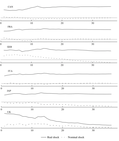
Figure 1.A. Response of real exchange rates (RER) to real and nominal shocks: Advanced economies Sample period 1973:1-1990:12 0 10 20 30 CAN 0 10 20 30 FRA 0 10 20 30 GER 0 10 20 30 IT A 0 10 20 30 JAP 0 10 20 30 UK R l h k N i l h k 20

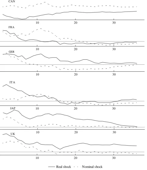
Figure 1.B. Response of real exchange rates (RER) to real and nominal shocks: Advanced economies Sample period 1991:1-2000:1 0 10 20 30 CAN 0 10 20 30 FRA 0 10 20 30 GER 0 10 20 30 IT A 0 10 20 30 JAP 0 10 20 30 UK R l h k N i l h k 20

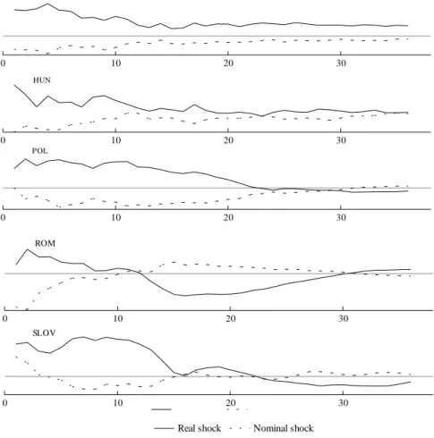
Figure 2. Response of real exchange rates (RER) to real and nominal shocks: Transition economies Sample period 1991:1-2000:1 0 10 20 30 CREP 0 10 20 30 HUN 0 10 20 30 POL 0 10 20 30 ROM 0 10 20 30 SLOV

Real shock Nominal shock 20

that has not accomplished an effective disinflation program (Wachtel and Korhonen, 2004).11

B. Impulse-response analysis

In this subsection, we use impulse-response analysis to study the effects of both types of shock on the endogenous variables in the SVAR models. For advanced economies, during the period 1973:1−1990:12, the results shown in Figure 1 suggest that real shocks cause a smooth increase in real exchange rates.12 _{Moreover, nominal}

shocks cause an unnoticeable effect on real exchange rates; thus, there is no evidence of overshooting. However, during the transition period, in general, nominal shocks tend to cause an increase in real exchange rates: there is some evidence in favour of overshooting.

For transition economies, in general, Figure 2 shows that the real exchange rate rises are due to real shocks. For the Czech Republic and Poland the real exchange rate depreciates smoothly in response to a nominal shock. For Romania we observe a more important depreciation of the real exchange rate in response to a nominal shock. Thus, for these accession economies there is evidence in favour of overshooting.

IV. Concluding remarks

This paper has analysed the sources of real exchange rate fluctuations for a set of advanced economies and Central and Eastern transition economies using the variance decomposition and the impulse-response analysis.

For advanced economies results suggest that there is evidence in favour of instability in the variance decomposition of the real exchange rates across samples. Thus, it seems that the sources of fluctuations of real exchange rates depend on the sample that we consider: for the period 1973:1−1990:12 real shocks appear to dominate nominal shocks and for the period 1991:1−2000:1, in general, nominal shocks play a central role in explaining fluctuations in exchange rates. Moreover,

11 _{As nominal exchange rates are managed during the transition period for transition economies,} we have computed the decomposition of real exchange rates and price levels too, as Dibooglu and Kutan (2001) suggest. Results hardly differ between models with regard to the real exchange rate. These results are available upon request.

we observe that nominal shocks seem to dominate real exchange rate fluctuations for the Euro Zone countries during the subperiod 1991:1−2000:1. This reveals the central role of the Single Monetary Policy for these countries. This result would imply that models which emphasize the importance of real shocks to explain the sources of fluctuations of the real exchange rate would be more suitable for the first subsample, while sticky price disequilibrium models would be more suitable for the second subsample.

For transition economies, the sources of fluctuations of real exchange rates depend on the transition economy under consideration. In particular, real shocks mostly explain movements in the real exchange rates for the Czech Republic, Hungary and Slovenia while nominal shocks play a central role in explaining the variance in the real exchange rate for Poland and Romania. Thus, as a result of diverse initial conditions, and fiscal and monetary policies in transition economies, real exchange rates in some economies are driven mostly by real shocks, while in others they are driven mostly by nominal shocks.

References

Balassa, Bela (1964), “The purchasing power parity doctrine: A reappraisal”, Journal of

Political Economy 72: 584-596.

Begg, David, László Halpern and Charles Wyplosz (1999), Monetary and Exchange Rate

Policies, EMU and Central and Eastern Europe (Forum Report of the Economic Policy

Initiative 5), London, CEPR.

Blanchard, Olivier and Danny Quah (1989), “The dynamic effects of aggregate demand and supply disturbances”, American Economic Review 79: 655-673.

Brada, Joseph C. (1998), “Introduction: Exchange rates, capital flows, and commercial policies in transition economies”, Journal of Comparative Economies 26: 613-620.

Broeck, Mark D. and Torsten Sløk (2001), “Interpreting real exchange rate movements in transition countries”, Working Paper 56, Washington, IMF.

Desai, Padma (1998), “Macroeconomic fragility and exchange rate vulnerability: A cautionary record of transition economies”, Journal of Comparative Economics 26: 621-641. Dibooglu, Sel and Ali Kutan (2001), “Sources of real exchange rate fluctuations in transition

economies: The case of Poland and Hungary”, Journal of Comparative Economics 29: 257-275.

Dornbusch, Rudiger (1976), “Expectations and exchange rate dynamics”, Journal of Political

Economy 84: 1161-1176.

Égert, Balázs (2002), “Estimating the impact of Balassa-Samuelson effect on inflation and real exchange rate during the transition”, Economic System 26: 1-16.

Enders, Walter and Bong-Soo Lee (1997), “Accounting for real and nominal exchange rate movements in the post-Bretton Woods period”, Journal of International Money and

Engel, Charles (1993), “Real exchange rates and relative prices. An empirical investigation”,

Journal of Monetary Economics 32: 35-50.

Engel, Charles (1999), “Accounting for U.S. real exchange rate changes”, Journal of Political

Economics 107: 507-538.

Engel, Charles and John Rogers (2001), “Violating the law of one price: Should we make a federal case out of it?”, Journal of Money, Credit and Banking 33: 1-15.

Halpern, László and Charles Wyplosz (1997), “Equilibrium exchange rates in transition economies”, International Monetary Fund Staff Papers 44: 430-461.

Halpern, László and Charles Wyplosz (2001), “Economic transformation and real exchange rates in the 2000’s: The Balassa-Samuelson connection”, unpublished manuscript, Hungarian Academy of Science and Graduate Institute of International Studies.

Johansen, Soren (1988), “Statistical analysis of cointegrated vectors”, Journal of Economic

Dynamic and Control 12: 231-244.

Johansen, Soren (1992), “Estimation and hypothesis testing of cointegration vectors in a Gaussian vector autoregressive model”, Econometrica 59: 1551-1581.

Lastrapes, William D. (1992), “Sources of fluctuations in real and nominal exchange rates”,

The Review of Economics and Statistics 74: 530-539.

Morales-Zumaquero, Amalia (2003), “The real exchange rate fluctuations puzzle: Evidence for advanced and transition economies”, International Business and Economics Research

Journal 2: 39-52.

Morales-Zumaquero, Amalia (2004), “Explaining real exchange rate fluctuations”, Working Paper 23, Sevilla, Centro de Estudios Andaluces.

Rogers, John. and Michael Jenkins (1995), “Haircuts and hysteresis: Sources of movements in real exchange rates”, Journal of International Economies 38: 339-360.

Samuelson, Paul A. (1964), “Theoretical notes on trade problems”, Review of Economics and

Statistics 46: 145-154.

Wachtel, Paul and Iikka Korhonen (2004), “Observations on disinflation in transition economies”, Working Paper 5, Finland, Bank of Finland.