Towards the estimation of equilibrium exchange rates for CEE acceding countries: methodological issues and a panel cointegration perspective

W O R K I N G PA P E R S E R I E S

N O. 3 5 3 / A P R I L 2 0 0 4

TOWARDS THE

ESTIMATION OF

EQUILIBRIUM

EXCHANGE RATES FOR

CEE ACCEDING

COUNTRIES:

METHODOLOGICAL

ISSUES AND A PANEL

COINTEGRATION

PERSPECTIVE

In 2004 all publications will carry a motif taken from the €100 banknote.

W O R K I N G PA P E R S E R I E S

N O. 3 5 3 / A P R I L 2 0 0 4

TOWARDS THE

ESTIMATION OF

EQUILIBRIUM

EXCHANGE RATES FOR

CEE ACCEDING

COUNTRIES:

METHODOLOGICAL

ISSUES AND A PANEL

COINTEGRATION

PERSPECTIVE

1

by Francisco Maeso-Fernandez

2

,

Chiara Osbat

3

and Bernd Schnatz

4

1 The views expressed in this study are those of the authors and do not necessarily reflect those of the ECB.The paper has benefited from

This paper can be downloaded without charge from http://www.ecb.int or from the Social Science Research Network electronic library at http://ssrn.com/abstract_id=533022.

© European Central Bank, 2004 Address

Kaiserstrasse 29

60311 Frankfurt am Main, Germany

Postal address

Postfach 16 03 19

60066 Frankfurt am Main, Germany

Telephone +49 69 1344 0 Internet http://www.ecb.int Fax +49 69 1344 6000 Telex 411 144 ecb d

All rights reserved.

Reproduction for educational and non-commercial purposes is permitted provided that the source is acknowledged. The views expressed in this paper do not necessarily reflect those of the European Central Bank.

The statement of purpose for the ECB Working Paper Series is available from the ECB website, http://www.ecb.int.

C O N T E N T S

Abstract 4

Non-technical summary 5

1. Introduction 7

2. Methodological issues and review of

the literature 8

2.1 The country-by-country approach 8

2.2 The cross-section approach 1 1

2.3 The panel data approach 1 1

3. A cross-section analysis 1 3

4. Taking a panel cointegration perspective 1 5

4.1 Econometric strategy 1 5

4.1.1 Unit root tests 1 6

4.1.2 Cointegration tests 1 7

4.1.3 Estimation and inference in dynamic heterogeneous panel models 1 7

4.2 Estimation results 2 0

4.2.1 Data and unit root tests 2 0 4.2.2 Panel data results – bivariate

regressions 2 1

4.2.3 Additional fundamentals 2 3 4.2.4 Panel data results – multivariate

regressions 2 5

5. Out-of-sample extrapolation (“simulation”) stage: Some methodological considerations 2 7

6. Conclusions and outlook 2 9

Annexes 3 1

Bibliography 3 5

Abstract: This paper provides a discussion of methodological issues relating to the estimation

of the long-run relationship between exchange rates and fundamentals for Central and Eastern European acceding countries, focusing on the so-called behavioural equilibrium exchange rate (BEER) approach. Given the limited availability and reliability of data as well as the rapid structural change acceding countries have been undergoing in the transition phase, this paper identifies several pitfalls in following the most straightforward and standard econometric procedures. As an alternative, it looks at the merits of a two-step strategy that consists of estimating the relationship between exchange rates and economic fundamentals in a panel cointegration setting – using a sample which excludes acceding countries – and then “extrapolating” the estimated relationships to the latter. While focusing on the first step of such a strategy, the paper also delves into discussing technical aspects underlying the “extrapolation” stage. As a result, the paper endows the reader with the methodological and empirical ingredients for computing equilibrium exchange rates for acceding countries, providing estimates for the long-run coefficients between real exchange rates and economic fundamentals and a discussion of how to apply these results to acceding countries data.

JEL codes: C23, F31.

Non-technical summary

This paper provides a discussion of methodological issues relating to the estimation of the long-run relationship between exchange rates and fundamentals for Central and Eastern European acceding countries. Assessing exchange rate developments in relation to their “fair level” is conceptually difficult, as one needs to rely on a wide set of indicators and a broad range of models. Accordingly, various concepts of “equilibrium exchange rates” may serve as a helpful tool to address the issue of the appropriate level for a currency. Estimating such equilibrium exchange rates is a challenging task for major currency pairs and is even more complicated for the exchange rates of acceding countries, on account of substantial problems in terms of data availability and measurement as well as difficulties in choosing an appropriate econometric methodology. Moreover, as these countries were in transition within the short time span for which data are available, their equilibrium exchange rate may have undergone rapid change in itself, further complicating the assessment. Indeed, the sizeable and in some cases massive real appreciation of acceding countries’ currencies may reflect, to a large extent, this transition to a market economy.

One contribution of this paper is to review the merits and disadvantages of several strategies that have been proposed and carried out in the empirical literature. For instance, while a country-by-country analysis is intuitively the most straightforward strategy, it can be subject to drawbacks in terms of interpretation of the results. This is mainly due to data problems and the particularity of the transition period. First of all, the length of the sample in these studies is rather short, commonly spanning a period of around 10 years. Second, the econometric techniques used (unit root and cointegration tests) can be severely biased in such small samples. Third, and more importantly in this case, the estimated equilibrium level crucially depends on the estimated intercept, which will be biased due to the particularity of the transition process. Moving to a panel data framework including only acceding countries (or a sub-set of these countries) does not solve the problem of biased estimates. In order to avoid such problems, in the first part of the paper we assess the relationship between productivity advances and real exchange rate developments in a simple cross-section context.

However, as this method has the drawback that it ignores the time series information contained in the data, in the second part of the paper we look at the merits of a two-step strategy in the tradition of a “behavioural equilibrium exchange rate” (BEER) framework. The first step of the method consists of estimating the relationship between exchange rates and economic fundamentals in a panel cointegration setting, using a sample that excludes acceding countries. Then, in the second step, we propose “extrapolating” the estimated relationship to each acceding country. While focusing on the first step of such a strategy, the paper also delves into discussing technical aspects underlying the “extrapolation” stage. As a result, the paper endows the reader with the methodological and empirical ingredients for computing equilibrium exchange rates for acceding countries, providing estimates for the long-run coefficients between real exchange rates and economic fundamentals and a discussion of how to apply these results to acceding countries data. Although not purged of shortcomings, given its relatively ad hoc nature, the proposed two-step approach has the advantage that combining the different econometric methodologies and the different calibrated constant terms could give an array of point estimates for the equilibrium exchange rate for each country.

The core of the paper is constituted by the estimation of long-run relationships between the exchange rate and fundamentals using annual data for 25 OECD countries between 1975 and 2002. As panel unit root tests suggest that the underlying data are non-stationary, they must be modelled in a suitable econometric framework in order to avoid drawing conclusions based on spurious results. After confirming the presence of cointegration among the variables, we consider three main approaches to estimating a long-run relationship in a panel framework: the Pooled Mean Group estimator advocated by Pesaran et al. (1997), Dynamic OLS – as suggested by Kao and Chiang (2000) and Mark and Sul (1999 and 2000) – and finally Fully-Modified OLS estimators as proposed by Pedroni (1999, 2000 and 2001). The results indicate that in the medium to long term the real exchange rate depends on developments in relative per-capita income (as a measure of productivity), relative government spending and relative openness. While higher per-capita income and government spending give rise to an equilibrium appreciation of the currency, an increase in openness is associated with equilibrium depreciation.

1.

Introduction

With the completion of the negotiations on EU accession, ten countries will join the European Union in May 2004 as members with a derogation. These countries will eventually adopt the euro, upon reaching a high level of sustainable convergence as spelled out in the Maastricht treaty. Directly after EU accession, each member state will treat exchange rate policy as a “matter of common interest” and, in principle, will have the option to participate in the ERM II. For doing so, it is necessary to reach a multilateral agreement on a sustainable central parity for the exchange rate of new members’ currencies vis-à-vis the euro. Assessing exchange rate developments in relation to their “fair level” is conceptually difficult, as one needs to rely on a wide set of indicators and a broad range of models. In this context, various concepts of “equilibrium exchange rates” may serve as a helpful tool to address the issue of the appropriate level for a currency. Estimating such equilibrium exchange rates is a challenging task for major currency pairs and is even more complicated for the exchange rates of acceding countries, on account of substantial problems of data availability and measurement as well as difficulties in choosing an appropriate econometric methodology. Moreover, as these countries were in transition within the short time span for which data are available, their equilibrium exchange rate may have undergone rapid change in itself, further complicating the assessment.

Indeed, the sizeable and in some cases massive real appreciation of acceding countries’ currencies may reflect to a large extent this transition to more market-oriented economies. Since 1993, the Baltic countries faced the strongest real appreciation. The external value of the Estonian and Latvian currencies more than doubled in real terms (CPI-based) and in the extreme case of Lithuania the rise in the real exchange rate amounted to more than 600%.1 _In

these countries, the pace of the real appreciation was very high up to 1997 and moderated thereafter. In comparison to the Baltic States, the increase in the real external value of the currencies of the Czech Republic, Poland and Slovakia since 1993 was smaller but still substantial. In Hungary, the real exchange rate of the forint appreciated steadily between 1995 and 2002, apart from a period of depreciation during the Russian crisis. By contrast, the real appreciation of the Slovenian tolar was more moderate.

This paper focuses on a so-called behavioural equilibrium exchange rate (BEER) approach and presents an empirical analysis of the long-run relationship between exchange rates and fundamentals based on panel cointegration techniques. On account of limitations of standard econometric models when applied to acceding countries’ currencies, this paper looks at the merits of a two-step approach. The first step involves the estimation of long-run relationships between the real exchange rate and economic fundamentals, using data from non-acceding OECD countries (“estimation stage”). The second step involves the derivation of an “equilibrium real exchange rate” as a function of these economic fundamentals using data from acceding countries (“extrapolation” stage).2 _{This paper focuses on the first step and}

1 _{Overall, the change in the real exchange rate on the basis of producer prices was lower but in most countries}

still significant.

2 _{Unlike other contexts, in the context of this paper, the term “extrapolation” should not be intended as an}

out-of-sample exercise along the temporal dimension, but as an application of the estimated coefficients out of sample across the cross-sectional dimension.

discusses the extrapolation stage only at a methodological level. Accordingly, the paper should be understood as a kind of a guide, providing the procedural steps to compute “equilibrium” exchange rates for acceding countries. In this context, we provide estimates for the long-run equilibrium coefficients between economic fundamentals and real exchange rates and a discussion of how to apply these results to acceding countries data.

The paper is structured as follows: The next section briefly discusses some fundamental methodological issues with a special emphasis on the BEER approach and provides a selected overview of the academic literature on this topic. Section 3 presents a simple cross-section analysis, which focuses on the relationship between productivity advances and exchange rate developments. Section 4 extends this analysis by applying panel cointegration techniques. Moreover, it broadens the perspective by introducing additional macroeconomic fundamentals, which could be relevant for the determination of equilibrium exchange rates. Section 5 discusses technical aspects underlying the second stage (so-called “out-of-sample” approach). Section 6 concludes.

2.

Methodological issues and review of the literature

The literature on acceding countries’ exchange rates has employed different concepts of equilibrium exchange rates, from the fundamental equilibrium exchange rate (FEER) approach (see, e.g. Šmídková et al. (2002) as well as Coudert and Couharde (2002)) to the

monetary model (see Crespo-Cuaresma et al. (2003)) to the BEER approach. The focus of

this paper is on the BEER, which constitutes a more empirical approach to modelling the relationship between real exchange rates and various economic fundamentals.3 _{Overall, the}

available empirical BEER studies on acceding countries’ equilibrium exchange rates can be classified into three categories (as illustrated in Chart 1): a) studies which estimate equilibrium exchange rates on a country-by-country basis,4 _{b) cross-section analyses and c)}

studies based on panel data, which exploit simultaneously the cross-section and the time series information contained in the data. The merits and limitations of these approaches are briefly addressed below.

2.1

The country-by-country approach

Carrying out country-by-country analyses is intuitively the most straightforward strategy, as the equilibrium exchange rate is estimated for each country, taking into account the peculiarities of each individual economy. However, this approach could be subject to drawbacks in terms of interpretation of the results, due to data problems and the particularity of the transition period.

3 _{Different concepts for assessing exchange rates are discussed in ECB (2002a) and in MacDonald (2000).}

Obviously, the BEER is only one of the methods that could be employed. Using the FEER or a NATREX model could be considered as an alternative, but a thorough assessment on the basis of alternative methodologies is beyond the scope of this paper.

4 _{For instance, Jakab and Kovacs (2000) estimate the relationship between economic fundamentals and the}

Hungarian forint in a SVAR framework. Egert (2002) estimates the relationship between economic fundamentals and the real exchange rate of individual CEE countries, but also shows results of a panel test. Similarly Rahn (2003) estimates both country-by-country and panel regressions.

Chart 1: Methodological issues in choosing an appropriate econometric strategy in a BEER framework Ø Short sample Ø Data properties Ø Biased estimates Country-by-country analysis

Ø Missing time series dimension Cross section analysis Including only AC Ø Biased estimates “In-sample” approach Including AC plus

a broad set of other countries

Ø Biased constant term

Ø Heterogeneity

Panel data analysis

Ø No constant for AC “Out-of-sample” approach Including only other countries (excluding AC) and then applying estimated relationship to AC.

First of all, the length of the sample in these studies is rather short, commonly spanning a period of around 10 years as it would be futile to include data reaching back to the 1980s when these countries were still operating in a planned-economy environment. Since the real exchange rate and the underlying macroeconomic fundamentals are commonly found to be non-stationary variables, cointegration analysis is often employed. However, cointegration

test statistics and estimates are strongly biased in such small samples. The fluctuations of real exchange rates can exhibit rather long-lasting swings, so that it could well be that even a sample period of ten years fails to reflect broad movements around some equilibrium schedule. Importantly, some studies have suggested that acceding countries’ exchange rates have converged gradually from an initial substantial undervaluation towards their equilibrium level in the 1990s.5 _{Accordingly, the actual exchange rates might have gradually approached}

the equilibrium level after their strong devaluation at the beginning of the reform process and it cannot even be ruled out per se that they may have not reached this equilibrium value yet. If this possibility is not properly accounted for, some of the ensuing coefficient estimates (in particular, the estimate of the intercept) could be biased.

Chart 2 provides a very stylised illustration of this point. It shows a typical pattern for acceding countries’ real exchange rates over the last twelve years (bold solid line).6 _{At the}

early stage of transition, these currencies appreciated strongly, to increasingly level off in recent years. If the correct path of the equilibrium exchange rate is given by the thin black solid line, the exchange rate was initially undervalued but converged over time to more “reasonable” levels and has been close to its equilibrium or even slightly overvalued in recent years.7 _{The equilibrium exchange rate is assumed to gradually appreciate, for example owing}

to higher productivity gains in acceding countries compared with the euro area. If one simply estimates a cointegration model linking the real exchange rate to productivity on a country-by-country basis, without taking the initial period of undervaluation into account, one would expect the constant term to be biased (dotted line). This would give rise to misleading results for the evaluation of the exchange rate level.

In order to account for a gradual adjustment of the initially undervalued currency towards equilibrium, Krajnyak and Zettelmeyer (1998), e.g., explicitly address the issue of adjustment to equilibrium from an undervalued position by including in their panel data analysis a time-varying “transition dummy”. However, if the coefficient on the transition dummy is the same for all countries, it reflects only the average extent of “undervaluation” of these currencies, although the adjustment path may have been rather diverse. As an alternative, one could consider including a “transition variable”, which could be shaped for example like a logarithmic trend, on a country-by-country basis. Experimenting with such an approach, however, we found an over-fitting of the equilibrium schedule, which amounts to finding by construction that the currencies are close to their equilibrium at the end of the sample, independently of how much they have appreciated in the past.

5 _{See Halpern and Wyplosz (1997) as well as Krajnyak and Zettelmeier (1998). As this analysis is built on real}

dollar wages, it is difficult to draw strong conclusions for the euro exchange rates of CEE currencies. It also needs to be emphasised that between 1995-2002, the real appreciation of the currencies of CEE countries was stronger against the euro than against the US dollar. However, these studies raise the awareness that such an eventuality needs to be taken into account in choosing an appropriate econometric strategy. Darvas (2001), by contrast, suggests that Hungary did not start the transition period with a substantially undervalued currency.

6 _{The series is constructed as an unweighted average of accession countries’ real exchange rates between 1993}

and 2004. Forecasts provided by the AMECO database were used for the end of the sample.

7 _{The series was constructed using the trend in per capita income of accession countries relative to the euro area,}

multiplied by an elasticity of 0.5. The level is set ad hoc to illustrate a situation of an exchange rate which is broadly in line with fundamentals in recent years.

Chart 2: Illustration: Estimating an appreciating equilibrium exchange rate

Index; number of years on the horizontal axis

100 120 140 160 180 200 220 1 2 3 4 5 6 7 8 9 10 11 12

actual equilibrium estimate

2.2

The cross-section approach

Instead of employing a time series approach, one could employ a cross-section regression, to avoid the problems outlined above regarding the data properties. This strategy is often followed when analysing equilibrium exchange rates of acceding countries in a more illustrative setting, mainly based on graphical analysis. Such an approach follows, in principle, Kravis et al. (1982) and use US-dollar based purchasing power parity conversion factors provided by the International Comparison Programme of the University of

Pennsylvania or data provided by Eurostat.8 _{These papers commonly explain, in a}

cross-section context, the gap between this PPP exchange rate and the actual exchange rate (the so-called “exchange rate gap”) on the basis of per capita income (in dollar or euro PPP terms). An analogous approach for the euro is employed in section 3 of this paper.

2.3

The panel data approach

More sophisticated studies have employed panel data models in order to overcome the problem of short time series.9 _{These papers can be separated into studies following either an}

“in-sample” or an “out-of-sample” approach (see Chart 1). The “in-sample” approach usually

8 _{This approach has been employed by DeBroek and Sloek (2001) in the first part of their paper, Randveer and}

Rell (2002) in an analysis for Estonia, and Brook and Hargraeves (2001) in an analysis for New Zealand. Cihak and Holub (2003) discuss this approach very comprehensively. They also carry out a similar exercise from a Czech perspective controlling – albeit rather ad hoc – for other variables.

9 _{See, for instance, DeBroek and Sloek (2001) and Fischer (2002). Rahn (2003) employs a “in-sample” panel}

cointegration framework for effective exchange rates of acceding countries and derives equilibrium exchange rates on the basis of a algebraic transformation along the lines of Alberola et al. (1999). He finds that acceding countries’ currencies may be substantially overvalued.

focuses on the panel including only acceding countries (or a sub-set of these countries) and has the advantage that the cross-section sample is fairly homogeneous. However, such a procedure may entail similar drawbacks as the country-by-country approach, leading to biased estimates of the deviations from equilibrium. Adding more countries which were not subject to the transition process could mitigate the problem of a bias in the estimates, but the constant terms may still be distorted towards finding an overvalued exchange rate.

As an alternative, an “out-of-sample” approach is based on a two-step procedure for

estimating equilibrium exchange rates for acceding countries. In the first step, the equilibrium exchange rate is estimated for non-acceding countries. In the second step, equilibrium exchange rates for acceding countries are then “extrapolated” on the basis of the estimated structural relationships. In this context, the choice of the cross-section coverage requires a compromise between maximising the degrees of freedom in the estimation by including as many countries as possible and maintaining a reasonable degree of sample homogeneity. Halpern and Wyplosz (1997) and Krajnyak and Zettelmeier (1998) for instance, employed this approach and opted for a very broad country coverage, using a sample of 85 industrialised, developing, planned and transition economies. While a broad panel may be useful in identifying more general patterns, which were less dented by the transition process itself, it also amplifies the problems related to heterogeneity, as countries as diverse as the United States, the Netherlands, Japan, Myanmar, Papua New Guinea and Zimbabwe are combined. Both papers employ static regressions including a broad set of economic fundamentals. However, this does not take the time series properties of the data properly into account, as the data are in all likelihood non-stationary. Using fewer data points in the time dimension (five-year intervals), as done in these studies, does not overcome this limitation.10

In this context, both the sample selected and the econometric approach followed by Kim and Korhonen (2002) appear to be more compelling. They employed data from 29 middle and high income countries, arguing that the acceding countries share common characteristics with both groups: while their per capita GDP is more similar to middle-income countries, their industrial and trade structure is more similar to high-income countries. They derive equilibrium exchange rate indices, both against the US dollar and in effective terms, for five acceding countries.

In the “out of sample” approach, the estimation stage would be followed by an extrapolation stage. In this second step, the fitted value for the exchange rate is calculated on the basis of the acceding country’s data using the point estimates of the long-run parameters estimated in the previous step and it is interpreted as the equilibrium exchange rate for each acceding country. The derivation of an appropriate “equilibrium exchange rate” is, however, far from trivial. Apart from controlling for changes in economic fundamentals affecting the “equilibrium exchange rate” over time, in order to provide a guide about the appropriateness

10 _{Halpern and Wyplosz (1997) use for sample covering 1970 to 1990 observations every five years. They find a}

specification including, as exogenous variables, GDP per worker, school enrolment, the share of agriculture relative to industry, the share of the government sector, and the inflation rate, which, in their original paper, are statistically significant according to standard critical values. As this study estimates a model based on a panel data set excluding acceding countries for the period 1975 to 1990 and applies estimates to acceding countries for the period after 1990, this can be interpreted as a “double” out-of-sample exercise. In an update of their paper (Begg et al. (1999)), after including one more data point for 1995 for each country, some of these fundamentals become insignificant while others, such as demographic factors, trade openness and external indebtedness, become important. On the whole, this may point to some stability problems in this approach.

of the current level of the exchange rate, one needs to choose an appropriate constant term too. The latter is estimated with a bias in “in-sample” regressions and cannot be estimated directly in “out-of-sample” exercises. Section 5 discusses some methodological issues involved in choosing a constant term in such exercises.

3.

A cross-section analysis

This section presents an assessment of the relationship between real exchange rates and fundamentals, based on a cross-section approach using data on PPP exchange rates against the euro as provided by the European Commission’s Ameco database (See Annex 1 for the data sources). The PPP exchange rate is defined as the number of units of a country’s currency required to purchase the same basket of goods in that country as one unit of the numeraire currency would buy in the numeraire country. Accordingly, PPP exchange rates are commonly used as conversion factors, which allow cross-country comparisons of economic aggregates in real terms. For instance, for the Czech koruna against the euro the PPP conversion factor is defined as the number of koruna needed in the Czech Republic to buy the same basket of goods and services as one euro would buy in the euro area. In 2002, the PPP exchange rate of the Czech koruna was CZK/EUR 15.18, while the actual euro-koruna exchange rate was CZK/EUR 30.8. This implies that the real value of the Czech currency is almost 50% lower in the euro area than in the Czech Republic. This mainly results from the fact that prices of non-traded goods and services are much higher in the euro area than in the Czech Republic (while traded goods should have more similar prices in both countries). On the basis of this concept one can compute so-called “exchange rate gaps”, defined as the ratio of the PPP exchange rate and the actual exchange rate. In a time series context, they have the same pattern as real exchange rate indices, but PPP exchange rates have the advantage of being meaningful in levels. Chart 3 shows these gaps for 38 industrialised countries, emerging markets and the accession countries in 2002. For the CEE acceding countries, the gaps are strongly negative, ranging from –0.33 for Slovenia to more than –0.60 in the case of Slovakia. In this sample, only Bulgaria and Romania have larger exchange rate gaps. For Malta and Cyprus, exchange rate gaps are smaller than for some euro area countries, such as Portugal or Greece, and comparable with Korea and Spain. At the other end of the spectrum are countries such as Japan and Switzerland, where the cost of living is much higher than in the euro area. Overall, this indicates that the purchasing power of CEE acceding countries’ currencies is much lower in the euro area than in their home countries. The presence of higher non-traded goods and services prices in one country relative to another country – given traded good prices – is often related to the Balassa-Samuelson theory, according to which relative prices of non-traded and traded goods in each country are inversely related to the relative productivity in the two sectors.11 _{In a nutshell, since traded}

goods sector productivity can be assumed to be higher in industrialised countries, non-traded

11 _{In practice, the differentiation between traded and non-traded goods is an artificial simplification. While the}

general pattern that prices of non-traded goods are lower than prices of traded goods seems to prevail, in Central and Eastern European countries, for instance, the price of semi-durable goods and food is also sizeably lower than in the EU. Accordingly, the real appreciation experienced by acceding countries’ currencies in recent years may also reflect price increases in the tradable sector. We are grateful to the anonymous referee for pointing this out.

goods prices are also higher there. In addition, the relative price between non-traded and traded goods is influenced by demand-side factors as well as price regulation and tax policies. Demand effects may arise, for instance, from non-homothetic preferences when the demand for non-traded services, which are more likely to have luxury good characteristics, increases with prosperity (see Bergstrand (1991)). Regarding the possible effect of government inference, Cihak and Holub (2003) cannot find a statistically significant relationship between the exchange rate gap and several fiscal variables in a similar cross-section analysis. By contrast, they find the size of agricultural employment as being significant. This is interpreted as a proxy for the political temptation to government inference in this sector, which may in turn have an impact on food prices.

Chart 3: Exchange rate gap in 2002

-0.8 -0.6 -0.4 -0.2 0 0.2 0.4 0.6

Source: ECB and AMECO

Overall, the “exchange rate gap” (egap henceforth) should be farther in negative territory, the lower the level of productivity and the stage of a country’s economic development. To account for the Balassa-Samuelson and demand effects, two explanatory variables, which should show a positive link with the exchange rate gap, have been constructed. The first is economic development, measured as GDP per capita in PPP terms (ypc)12 _{and the second is a}

productivity variable, measured as GDP in PPP terms divided by the number of persons

employed (prod).13 _{Average labour productivity (ALP) and per capita income are highly}

correlated by construction and cannot be used in the same regression to disentangle the relative importance of supply and demand side factors. In order to avoid the influence of the

12 _{This follows seminal work by Kravis et al. (1982) and it is what Samuelson (1996) called the “Penn effect”.}

Using per-capita income may also better reflect the fact that the relative price between non-traded and traded goods is also influenced by demand-side factors.

13 _{On purely theoretical grounds, total factor productivity (TFP), which signals improvement in the overall}

efficiency of the economic process, is the favoured measure of productivity. From a practical point of view, however, TFP cannot be measured directly and is difficult to estimate, particularly for accession countries (see Dobrinsky 2003, for a critical discussion and computation of TFP for acceding countries). As regards inputs in ALP, limited data availability for many countries rules out the use of output per hour worked. Therefore, output per person employed is commonly used in this literature. In order to account for diverging trends in productivity in the traded and in the non-traded goods sectors, several studies (see Fischer (2002), DeBroek and Sloek (2001)) have employed productivity measures in different sectors of the economy, e.g. agriculture, industry, and services. These data, however, are not consistently available for a broad cross-section of countries, so that we essentially assume that productivity advances materialise primarily in the traded goods sector and focus on economy-wide productivity measures.

transition trend present in acceding countries’ data on the estimation of the equilibrium, the regression was run by excluding the acceding countries.14 _{The OLS cross-section estimation}

results for 2002 are summarised below (t-statistics in parentheses).

2 ( 7.78) (7.62) ln(egap) 1.56 0.50ln(ypc) N 25,R 0.65 − = − + = = (1.1) 2 ( 4.62) (4.57) ln(egap) 1.93 0.48ln(prod) N 24, R 0.36 − = − + = = (1.2)

There is a significant positive relationship between the exchange rate gap and per-capita income as well as productivity. Overall, the results using per-capita income are stronger and more robust than those based on ALP as the t-statistics and the goodness-of-fit (measured by the adjusted R2_{) are markedly higher.}15 _{The results of this exercise depend to a significant}

extent on the group of countries included. While the elasticities presented in DeBroek and Sloek (2001) are broadly in line with these results, Coudert and Couharde (2003), for instance, find a lower goodness-of-fit and elasticity (0.25) in a similar regression based on income per capita including 120 developing and emerging countries. Experimenting with a broader country sample from the World Developments Indicators, we found that the inclusion of poor countries – particularly African countries – tends to generate lower elasticities. Nonetheless, it could be argued that the integration of these countries in international financial and goods markets is fairly limited so that it might be more sensible to include only countries with a reasonable degree of global integration.

While such a cross-section analysis provides a simple indication of the relationship between the exchange rate and income/productivity across countries, it has the drawback that it ignores the time series information contained in the data. In order to incorporate this information, one needs to adopt a panel data modelling approach. The analysis of the time series characteristics of the data indicates the presence of unit roots. As a consequence, the bivariate relationship between per-capita income and the exchange rate gap is estimated in a panel cointegration framework. Subsequently, we discuss the inclusion of other macroeconomic fundamentals in the model.

4.

Taking a panel cointegration perspective

4.1

Econometric strategy

The panel data perspective adds the time series dimension to the cross-section analysis of the previous section. While this increases the information set, it also complicates the analysis, as

14 _{The following 25 countries have been included: Australia, Austria, Belgium, Canada, Germany, Denmark,}

Finland, France, Greece, Ireland, Iceland, Italy, Japan, Korea, Mexico, Netherlands, Norway, New Zealand, Portugal, Spain, Sweden, Switzerland, Turkey, United Kingdom, United States. Since productivity data for Mexico was not readily available from the AMECO database, the second regression comprises only 24 countries.

15 _{Including the acceding countries in the regression increases the estimated elasticities significantly. In the}

cross-section regression excluding the acceding countries an increase of per-capita income relative to the euro area of 1% translates into an appreciation of almost 0.5%. In the regression including acceding countries the elasticity rises to almost 0.7%. For productivity, the corresponding elasticity is somewhat lower if the acceding countries are included and higher if they are excluded.

the time series characteristics have to be taken properly into account. It has been widely recognised that the real exchange rates as well as the underlying fundamentals are mostly non-stationary variables, which must be modelled in a suitable econometric framework in order to avoid drawing conclusions based on spurious results. Accordingly, we first test for unit roots in order to confirm that the variables are indeed integrated. We then test for cointegration and estimate the long-run parameters.

4.1.1 Unit root tests

Testing for unit roots in panel data instead of individual time series entails the advantage of increasing the power of the test by exploiting simultaneously cross-section and time series information. Furthermore, the test statistics conveniently converge asymptotically to the standard normal distribution. We carried out panel unit root tests on the basis of two standard test procedures: the Im et al. (2003) test (IPS t-test), which tests the null hypothesis of a unit root, and the test proposed by Hadri (2000), which has stationarity as the null hypothesis. The structure of the IPS t-test is based on N augmented Dickey-Fuller regressions:

1 1 for t = 1 T; i = 1, N, i p it i it ij it j i i it j y

ρ

y ₋

ϕ

y ₋

α γ

t

ε

= ∆ = +

å

∆ + + + K K (1.3)

where T is the length of the sample, N is the cross-section dimension, yit is the variable under

consideration, the term following the sum includes lagged dependent variables with country-specific lag length pi, αi and γi are country-specific intercepts (fixed effects) and trend

parameters, respectively. The error term εit is distributed as a white-noise random variable,

with possibly different variance for each member of the panel. The crucial coefficient for testing for a unit root is ρi. In contrast to the test proposed earlier by Levin et al. (2002), the

IPS t-test allows for heterogeneity in the value of ρi under the alternative hypothesis of

stationarity. This implies that the mean convergence dynamics are allowed to vary across the cross-section members. Hence the null hypothesis is H0: ρi = 0 for all i against the alternative

hypothesis Ha: ρi < 0. The IPS t-bar statistic is defined as the average of the individual ADF

statistics.16 _{After a suitable normalisation of the statistics using simulated values tabulated in}

Im et al. (2003), which account for the number of lags, the distribution of the test is standard normal.

The test proposed by Hadri (2000) is a residual-based Lagrange Multiplier test (LM) which – in the spirit of the KPSS test suggested by Kwiatkowski et al. (1992) – has a reverse null hypothesis, i.e. that the time series for each cross-section unit is stationary around a deterministic level or trend, against the alternative hypothesis of a unit root. It is based on the following regression: 1 T it i i it it t y

α γ

t u

ε

= = + +

å

+ (1.4)

16 _{Alternatively, Im et al. (2003) also propose an asymptotically equivalent LM-bar statistic. The results in this}

paper are, however, independent of the use of the t-bar or the LM-bar statistic so that the LM-bar is not discussed further.

where the deterministic terms are defined as in (1.3) above, and the error term has two components:

ε

_it, which is white noise, and

1 T it t u =

å

, which is a random walk. The test is based

on the fact that under the null hypothesis of stationarity the variance of the random walk

component ( 2

u

σ

) is zero. The test statistic takes the form

2 2

u

ε

σ

σ

, which has a standard normal

distribution under the null hypothesis.

4.1.2 Cointegration tests

The cointegration tests proposed by Pedroni (1999) have become a standard workhorse in panel data econometrics. As an alternative, the tests by Kao (1999) and McCoskey and Kao (1998) could be employed. However, the tests proposed by Pedroni allow for heterogeneous variances across the countries in the panel and some form of dependence across the countries at each point in time. Pedroni (1999) proposes seven residual-based tests based on the null hypothesis of no cointegration. The starting point is the group-by-group estimation of the proposed long-run relationship:

1 1 ...

it i i t it K Kit it

y = +

α γ

t+ +

θ β

x + +

β

x +

ε

(1.5)

where K is the number of regressors and βk are the elasticities. The deterministic elements (αi

and γi) are defined as above and θt are common time effects. This formulation allows for

considerable heterogeneity in the panel since fixed effects, individual-specific deterministic trends and different error variances are all allowed. Some of the Pedroni tests (the so-called group tests) also allow for heterogeneous slope coefficients, as the elasticities are estimated

by averaging the individual βk instead of pooling the long-run information. There is no

requirement for exogeneity of the regressors since the dynamics are determined jointly for both yi and all xki.

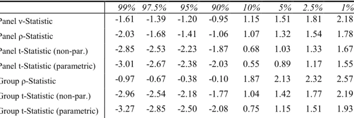
The seven tests proposed by Pedroni follow asymptotically a standard normal distribution after a suitable normalisation. A particularly important correction takes into account the heterogeneity of the cross-section units, by adjusting for the group-specific long-run variance of cointegration residuals. Four of the tests are based on pooling along the “within”-dimension of the panel and three are based on averaging along the “between”-“within”-dimension. Based on Monte Carlo experiments for a case with one dependent variable (Pedroni (1997)), the tests seem to have distorted size and low power for sample sizes below T=100 (see also Banerjee et al. (2003)). Overall, Pedroni (1997) suggests that the panel-ρ statistic seems to be the most reliable when T is large enough; for small T, the parametric group-t statistic and panel-t statistic appear to have the highest power, followed by the panel-ρ statistic. In view of this, we carried out some simulations to derive approximate small-sample critical values for the tests (see Annex 1).

4.1.3 Estimation and inference in dynamic heterogeneous panel models

We consider three main approaches to estimating a long-run relationship among integrated variables in a panel framework: (1) the error correction (EC) group and pooled mean-group estimators proposed by Pesaran et al. (1999), (2) the fully-modified OLS (FMOLS) and (3) the dynamic OLS (DOLS) estimators. The latter two estimators have been associated with

Pedroni (2000), Mark and Sul (2001) and Kao and Chiang (2000). The basic starting assumptions in all cases are that the variables are I(1), that they are cointegrated with the real exchange rate, but not among themselves, i.e., there is only one cointegration vector.

In the present context, the issue of slope homogeneity is particularly relevant. The strategy of estimating the relationships on the basis of a sample (N1) that excludes acceding countries and

then extrapolating to the sample of acceding countries (N2), requires slope homogeneity

between the two samples. Since this cannot be tested, a weaker requirement is to test whether

slope homogeneity holds at least for the countries in the N1 sample. This can be done by

computing both pooled and mean-group estimators. The pooled estimator estimates the long-run parameters jointly, thereby maximising the degrees of freedom. The mean-group estimator, by contrast, implies estimating the parameters country-by-country and then averaging them across countries. It provides consistent estimates of the mean of the long-run slope coefficients (though it suffers from a lagged dependent variable bias for small T), but it is inefficient if slopes are homogeneous. Under the null hypothesis of homogeneity the pooled estimator is consistent and efficient, while it is inconsistent under the alternative hypothesis. Using the fact that the mean-group estimator is always consistent, a Hausman test can be constructed to test for slope homogeneity.17

An important assumption of all panel cointegration tests considered in this paper is the absence of cross-sectional correlation. The possible presence of contemporaneous correlation can be addressed either by using time dummies or by subtracting the cross-sectional mean from the data. If the slopes are homogeneous, the two methods are equivalent. In the present paper, demeaned data were used for the pooled mean group estimator and time dummies were included for the other estimators.

Dynamic estimation: the error correction model.

Pesaran, Shin and Smith (1999) propose a pooled-mean group estimator (PMGE), which constrains the long-run coefficients to be identical in an error correction framework, but allow the short-run coefficients and error variances to differ across groups. They propose estimating the following autoregressive distributed lag (ARDL) model of order (pi, qi):

1 1 ' ' 1 _{1 0} i i p q it it i it _j ij it j _j ij it j i i it y

φ

y ₋

β

x ₌−

λ

y _{− =}−

δ

x ₋

α γ

t

ε

∆ = + +

å

∆ +

å

∆ + + + (1.6)

where yitis the dependent variable, xitis a m x 1 vector of explanatory variables, αi and

γ

i

represent the country-specific intercepts and time trend parameters respectively, λij and δij

include the country-specific coefficients of the short-term dynamics, εitis a white noise error

term. The long-run coefficients β are defined to be the same across countries. If фi is

significantly negative, there exists a long-run relationship between yitand xit. The equation is

17 _{Pesaran et al. (1999) also provide a likelihood ratio test for equality of error variances and/or slopes and claim}

that these tests usually reject the null of homogeneity. Therefore they suggest the Hausman test as an alternative. Pesaran et al. (1996) present two different ways to compute a Hausman test depending on how the variance of the mean group coefficient is obtained: either using a parametric or a non-parametric estimator. For the case of dynamic models, they find that the latter has better size properties than the former. However, using the non-parametric variance estimator does not guarantee a positive definite value for the difference between the variance of the mean group coefficients and the variance of the pooled ones. We are not aware of Monte Carlo studies about the properties of the different version of the Hausman test when other methods than the error correction are used.

then estimated using the maximum likelihood procedure to get the PMG estimator. This regression can also be estimated with individual specific βiwhich are then averaged over N to

obtain a mean-group estimator (MGE) which is the natural background to test for the presence of slope homogeneity based on a Hausman test.

Static estimation: FMOLS and DOLS

The starting equation to be estimated with these methods is the static regression (1.5). In a country-by-country set-up, this corresponds to the Engle-Granger procedure, which generates a consistent estimator of the long-run parameters. However, in the panel set-up, the long-run parameters are biased and Kao et al. (1999) show, on the basis of Monte Carlo experiments, that correcting the coefficients for this bias does not improve over the uncorrected OLS. This leads to using alternative methods, such as the FMOLS and the DOLS.

• FMOLS in panel data.

The FMOLS takes into account the presence of the constant term and the possible correlation between the error term and the differences of the regressors. To adjust for these factors, non-parametric adjustments are made to the dependent variable and then to the estimated long-run parameters obtained from regressing the adjusted dependent variable on the regressors. Accordingly, the FMOLS long-run coefficient estimators are defined as:

(

)

1

(

)

' ' * 1 1 ˆ ˆ it it T T i _t x xit _t x yit T i

β

=

å

₌ −

å

₌ −

λ

(1.7)

where y*_it are the regressands adjusted for the covariance between the error term and the

t

x

∆ and T

λ

ˆ is the adjustment for the presence of a constant term. The associated statistic for testing the significance of the parameters needs to be similarly adjusted. In the panel setting, the mean-group FMOLS long-run coefficients are obtained by averaging the group estimates

over N: 1 1 ˆ_FMOLS N ˆ MG N _i i

β

−

β

=

=

å

, and the corresponding t-statistic converges asymptotically to

a standard normal distribution: FMOLS 1/ 2 N₁ (0,1)

MG _i i

t =N−

å

₌t →N .

The pooled FMOLS coefficients can be computed in two different ways: weighted and unweighted. In the first case each group is weighted by the components of the long-run covariance of the group residuals and the right-hand-side variables in differences; in the second case these components are averaged. Pedroni (2000) shows that the weighted statistics require prior knowledge of the estimated parameters. Therefore, to compute a feasible weighted statistics several authors have proposed different starting values. Pedroni (2000) uses the values estimated under the null hypothesis, while Kao and Chiang (2000) employ the parameters from a static fixed-effects models. Mark and Sul (2001), for the case of DOLS, suggest to use parameters from an uncorrected DOLS estimation. Other alternatives proposed in the applied part of this paper include using as a preliminary step the estimate of the unweighted version of the tests and the mean group estimate, which is consistent but not efficient.

• DOLS in panel data

The starting point of the DOLS estimator is also equation (1.5). In order to obtain an unbiased estimator of the long-run parameters, DOLS involves a parametric adjustment to the errors of the static regression. The correction is achieved by assuming that there is a relationship between the residuals from the static regression and first differences of the leads, lags and contemporaneous values of the regressors in first differences:

*

q

it _{j q}c xij it j it

ε

=

å

₌₋ ∆ − +

ε

(1.8)

Substituting (1.8) into (1.5) yields:

*

1 1 1 1

q

it i i t i it i it _{j q} ij it j it

y = +

α γ

t+ +

θ β

x + +K

β

x +

å

₌₋ c x∆ ₋ +

ε

(1.9)

A simple OLS regression provides superconsistent estimates of the long-run parameters. The t-statistic is based on the long-run variance of the residuals instead of the contemporaneous variance, which is commonly used in OLS regressions. The group-mean DOLS are obtained in a similar fashion as the group-mean FMOLS. Similarly, weighted and unweighted versions of the DOLS estimator can be derived.

The decision to select one method over the other depends to some extent on the length of the sample (see Pedroni (2000)). In principle, FMOLS requires fewer assumptions and tends to be more robust. However, for the case of a single regressor, Kao and Chiang (2000) conclude that weighted DOLS has a smaller bias than weighted FMOLS. This result depends on the fact that both the number of lags used for kernels (in FMOLS) and the number of lags and leads in DOLS are fixed. Mark and Sul (2001) focus on DOLS and study the small sample performance of weighted and unweighted panel estimators and also of the mean group estimator. Most of the discussion relates to a model with only one regressor, although one specification with two regressors is also included. They suggest that (1) both panel methods outperform the mean group in terms of precision, and (2) the unweighted estimator tends to be more precise and displays smaller size distortion than the weighted estimator. Finally, Pedroni (2000) finds that group mean FMOLS has satisfactory size and power properties even for small panels if T is larger than N.

Since there is currently no paper available studying intensively and conclusively the small-sample properties of these tests based on Monte Carlo experiments, all methods will be employed in section 4.2 to ensure that the results are robust to the method chosen.

4.2

Estimation results

4.2.1 Data and unit root tests

The analysis is carried out on the basis of an annual balanced panel data set spanning the sample period 1975-2002 and includes the countries listed in footnote 14. The exchange rate

gap (egap) is defined as the purchasing power parity exchange rate divided by the market

(ypcr) for the total economy in the sample country (in PPP terms) relative to an euro area aggregate (see data Annex for details).18 _{Both variables are in logs.}

Table 1 summarises the unit root test results. For relative per-capita income, the IPS test fails to reject the null hypothesis of non-stationarity and, correspondingly, the Hadri test strongly rejects stationarity for this variable for specifications with and without trend. Accordingly, this variable is clearly non-stationary. For the exchange rate gap, the tests are also in favour of a unit root process, although the results are not as unequivocal. While the Hadri test again strongly rejects the null of stationarity for the exchange rate gap, the IPS test rejects the null of non-stationarity if there is no deterministic trend included in the regression. On the other hand, when a trend is included in the ADF regression, the IPS test fails to reject the null of a unit root. In the absence of information on whether the data generating process includes a non-zero constant term, one should include a deterministic trend in the ADF regression to ensure asymptotic similarity of the ADF t-statistic with respect to the deterministic coefficients. As a consequence, it seems reasonable to conclude on the basis of this result, and given the strong rejection of the Hadri test, that also the exchange rate gap follows a random walk.

Table 1: Unit root tests

IPS t-bar-test Hadri test

Variable no trend Trend no trend trend

Per capita income (ypcr) -0.29 -2.03 14.25 ** 8.22 **

Exchange rate gap (egap) 2.95 ** 0.39 14.41 ** 8.36 **

**/* Significant at the 1%/5% level. In the IPS-test, two lags have been imposed. The Hadri-test accounts for the presence of autocorrelated errors and employs the finite sample critical values following Hadri and Larsson (2002).

4.2.2 Panel data results – bivariate regressions

In view of the non-stationarity of the time series, it is important to employ a panel cointegration framework in order to avoid spurious regression problems, which – as shown by Entorf (1997), via simulation, and analytically by Kao (1999) – may lead to highly misleading statistics and potentially invalid conclusions. In the first step, the cointegration tests proposed by Pedroni (1999) are used to verify whether there is a long-run relationship between the exchange rate gap and per capita income. The results are summarised in Table 2.

In the majority of the cases the results point to cointegration between the exchange rate gap and per capita income. The null hypothesis is comfortably rejected in most cases, the exceptions being the non-parametric group-t statistic, which is, however, still fairly close to the 10% level, and the group-ρ statistic, which clearly fails to reject the null. This needs to be seen against the background of simulation evidence provided by Banerjee et al. (2003) showing that for panels of this dimension all tests suffer from significant size and power distortions, and in particular the group-ρ statistic is grossly undersized. However, the tests

18 _{It has to be kept in mind that the choice of benchmark country only affects the estimates of the fixed effects,}

while the estimates of the other coefficients are independent of this choice. The change in the estimated fixed effects is such that the fitted values from the estimated model will always be the same, whatever transformation is chosen.

performing best according to our Monte Carlo evidence – the panel-v and the panel-ρ statistic – suggest that the variables are cointegrated.

Table 2: Pedroni cointegration tests

Variables: egap, ypcr. N=25, T=28

test statistic p-value

Panel ν-Statistic 1.913 0.028

Panel ρ-Statistic -2.336 0.010

Panel t-Statistic (non-parametric) -2.310 0.010

Panel t-Statistic (parametric) -3.333 0.000

Group ρ-Statistic 0.261 0.603

Group t-Statistic (non-parametric) -1.014 0.155

Group t-Statistic (parametric) -2.872 0.002

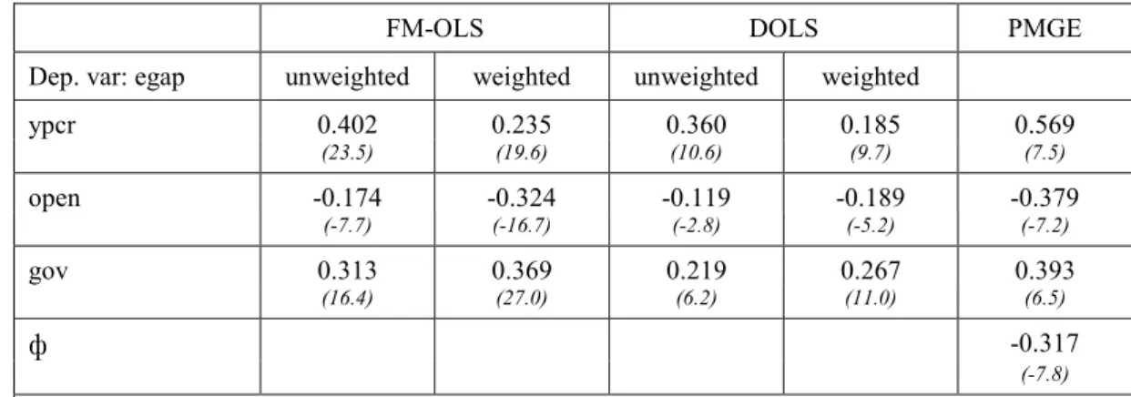
Given the evidence in favour of cointegration among the variables, the panel cointegration method discussed in the previous section can be employed to estimate the long-run parameters. Table 3 summarises the results.19

Table 3: Estimation results: (P)MGE, DOLS and FMOLS

FMOLS DOLS (P)MGE

Dep. var: egap unweighted weighted unweighted weighted pooled mean group

ypcr 0.634 0.484 0.386 0.571 0.436 0.740 (28.4) (33.0) (20.4) (29.3) (4.9) (3.3) ф -0.313 -0.373 (-14.7) (-14.8) Hausman-test 0.85 -0.04 1.21 0.00 2.20 p-value (0.357) na (0.271) (0.991) (0.14)

Note: The PMG was estimated using a ARDL (2,1) specification, for DOLS, 2 lags have been included. t-statistics in parentheses if not indicated otherwise.

The results broadly confirm those of the cross-section analysis. All estimators suggest that there is a highly significant and positive relationship between the exchange rate gap and per capita income. The coefficients are fairly close to those of the cross-section analysis, suggesting that an increase in per capita income of one percent feeds into a real appreciation – and thus (for lower income countries) a narrowing of the exchange rate gap – of between 0.39 and 0.63%. The significantly negative coefficients of the adjustment term (ф) in the PMGE strongly suggests mean reversion of the exchange rate gap to a long-term equilibrium schedule, and, thus, strengthens the evidence of cointegration among the variables. The

19 _{For the lag selection in the EC-PMGE, we first estimated a ARDL(2,2) specification and then removed}

insignificant lags from the dynamic specification in order to get a more parsimonious model. The DOLS estimates employ two lags and two leads. Overall, the results were very robust with respect to the choice of the lag structure. A country-specific constant has been incorporated while a time trend was not included.

magnitude of the coefficient implies a half-life of deviations from equilibrium of almost two years.

The results of the Mean-Group estimator (MGE) proposed by Pesaran et al. (1999) are reported in the right-hand-side column. These estimates provide indirect information about parameter heterogeneity in the sample and, thus, poolability of the data. The coefficients are broadly in line with those of the PMG estimator in terms of sign and magnitude. More formally, the Hausman tests cannot reject that the sample is sufficiently homogeneous to be pooled.20 _{As can be expected under these conditions, the significance of the coefficients}

increases noticeably when long-run homogeneity is imposed. The strong evidence in favour of slope homogeneity is quite important in view of the feasibility of the proposed two-step procedure. In-sample homogeneity could be seen as a necessary condition for extrapolation: it does not guarantee that the slopes would also be homogeneous if the sample of countries was enlarged, but indications of heterogeneity would clearly make the extrapolation untenable. Furthermore, even if the long-run parameters were not homogeneous between the transition and non-transition samples in the past, due to transition factors, it could still be appropriate to apply “post-transition” estimates to assess the present level of equilibrium exchange rates in transition countries.

In the country-specific regressions, the long-run elasticities of per capita income are somewhat dispersed, which is partly due to the limited degrees of freedom precluding an efficient estimation of the coefficients. For the MGE, they range from roughly –2 (insignificant) in the case of the United States to +3.2 in the case of Australia. In all but five cases, however, the coefficient has the correct sign and there is not a single case in which the coefficient is significantly negative. The goodness-of-fit (R2_{) is commonly below 50% and in}

all but four cases above 10%. At the 5% significance level, there is evidence for serial correlation in only one out of the 25 countries included in the sample. In three equations there seem to be some problems with the functional form, but there is not a single equation having non-normal errors and only for one country heteroscedastic errors seem to be present. The fact that 21 out of 25 country-specific equations show no evidence of misspecification is reassuring. The results for the FMOLS and DOLS are only slightly worse, as more groups have the wrong sign (seven and nine, respectively), while the dispersion of the parameter estimates across countries diminishes somewhat.

In addition, several robustness checks were carried out. Firstly, dropping the countries with the highest estimated coefficients to assess the dependence of the panel estimates on specific countries gives almost identical coefficients. Changes in the number of lags did neither alter the results. Finally, recursive regressions confirmed that the results were reasonably stable.

4.2.3 Additional fundamentals

Apart from productivity differentials, an array of variables has been included in model specifications for estimating equilibrium exchange rates.21 _{In the following, we pragmatically}

draw on the findings of this literature in the selection of additional variables.

20 _{The LR tests reject the restrictions including homogeneity at the 5% significance level, but not at the 1% level,}

which is rather encouraging since Pesaran et al. (1999) claim that it is almost impossible not to reject this hypothesis.

21 _{For a more thorough discussion of variables that can be included in a BEER framework, see MacDonald 2000,}

First of all, given the increasingly free flow of capital across borders, indicators reflecting the

international economic environment such as the real interest rate differential and

terms-of-trade shocks may be relevant. Both variables are, however, subject to measurement problems and data deficiencies, which are even more binding for economies in transition. For instance, data for terms of trade as well as for long-term interest rates are rather scarce. Moreover, a measure of real interest rates would need to include an assumption on inflation expectations, which is difficult to employ, particularly for emerging markets and the acceding countries.22

Whenever such variables were employed in empirical work related to acceding countries, the findings also were not very encouraging. For example, DeBroek and Sloek (2001) and Fischer (2002) include the terms of trade and various indices of commodity prices but generally fail to find a robust link with the real exchange rate. Moreover, commodity price shocks may affect countries differently, contingent on their resource dependency, making a pooled estimation of the terms-of-trade effects more difficult.

Regarding the domestic economic environment, variables related to the fiscal stance and

monetary policy considerations are frequently included as determinants of the real exchange

rate. Government spending relative to GDP is one variable typically included in such regressions. In practice, government spending may have different short-run and long-run effects on real exchange rate movements. In the short to medium run, a positive impact of government spending on the real exchange rate can be conceived, if the private sector lowers its demand for goods less than the increase in government spending, or if the marginal propensity of the public sector to spend on non-traded goods is higher. The latter possibility appears plausible, given the government sector’s spending on infrastructure, for instance, which is mainly satisfied by domestic inputs. Therefore, higher government spending could affect the real exchange rate positively via higher demand for non-traded goods. In the long term, however, higher government spending, in particular if deemed unbalanced, may lead to distortions in an economy and undermine the market’s confidence in a currency. On the other hand, particularly in acceding countries in recent years, public spending affected, to a sizeable extent, growth-enhancing effects such as human capital formation, infrastructure building and establishing an institutional environment supporting a proper functioning of the market economy. In the available empirical estimates, such growth-enhancing effects, in combination with the demand-side considerations, appear to dominate.23 _{On the financial sector side, two}

variables have been employed in the literature: money balances and credit growth. Given their ambiguous impact (as they may reflect expansive monetary shocks as well as financial deepening), neither DeBroek and Sloek (2001) nor Begg, Halpern and Wyplosz (1999) find a significant effect of such variables.

Moreover, taking a macroeconomic balance perspective, foreign indebtedness of a country is often assumed to be an important exchange rate fundamental (see e.g. Alberola et al 1999). However, data quality is an issue for such a variable. Compiling a net foreign asset variable in a consistent way is not straightforward. Frequently, accumulated current account positions have been used in the literature, but those data are only a very rough proxy of actual external indebtedness. Furthermore, in a BEER framework, including a external debt variable may raise new issues in terms of interpretation. For the OECD countries, one would indeed assume

22 _{However, omitting the real long-term interest differential might not be a crucial issue as, theoretically, this}

should be stationary, and thus, it should have a non-permanent impact on the BEER.

that higher indebtedness should translate into an “equilibrium” depreciation of the home currency. For acceding countries, by contrast, increasing indebtedness from very low initial levels may constitute a move towards an equilibrium debt level as the country builds its productive capacity. In such a case, it is less straightforward to anticipate the exchange rate effect. Moreover, while certainly a key variable from a standard theoretical point of view, previous work on bilateral euro exchange rates and the effective exchange rate suggested that net foreign assets may lead to inconclusive evidence (see Maeso-Fernandez et al. 2001). This finding was probably affected by the fact that the level of foreign debt may be a variable integrated of order larger than one. Therefore, it would be difficult to analyse it in a panel data framework.

Several authors also suggest that an increase in economic openness should have an influence on the real exchange rate. Similar to the government spending variable, there are arguments in favour of a positive or a negative impact on the real exchange rate. On the one hand, the more open to trade a country is, the less it relies on protection and distortions to its external accounts: hence increasing openness should enhance the country’s economic performance and lead to an appreciation of the real exchange rate. To some extent, this channel may already be captured by including a proxy for productivity developments. On the other hand, Edwards (1994) and Elbadawi (1994) derive an equilibrium exchange rate model for developing countries where it is shown that a greater openness to foreign trade leads to a real depreciation as a result of lower tariffs on imports or taxes on exports. The empirical evidence for this variable is broadly in favour of a significant negative impact on the real exchange rate.24 Against this background, two variables were added (in logs) to the model that links the exchange rate gap to per capita income: government spending as a ratio of GDP relative to the EU average (gov), and openness defined as the average of exports and imports of goods as a ratio of GDP (open), again relative to the EU average. The estimation procedure is the same as in the bivariate case.

4.2.4 Panel data results – multivariate regressions

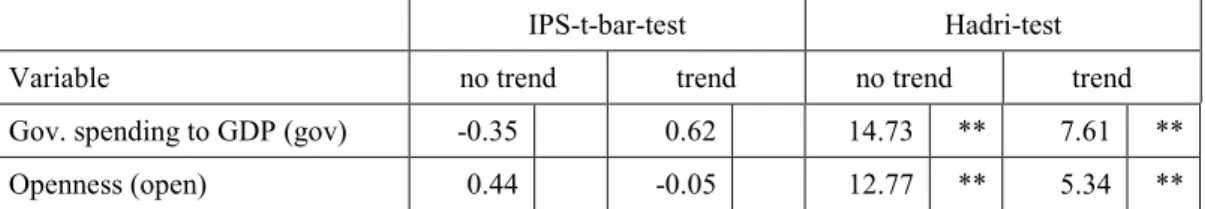
Tests for the order of integration of government spending and openness clearly suggest that both are random walks (see Table 4).

Table 4: Unit root tests

IPS-t-bar-test Hadri-test

Variable no trend trend no trend trend

Gov. spending to GDP (gov) -0.35 0.62 14.73 ** 7.61 **

Openness (open) 0.44 -0.05 12.77 ** 5.34 **

**/* Significant at the 1%/5% level. In the IPS-test, two lags have been imposed. The Hadri-test accounts for the presence of autocorrelated errors and employs the finite sample critical values following Hadri and Larsson (2002)

24 _{Kim and Korhonen (2002) and DeBroek and Sloek (2001) find strong evidence for a significantly negative}

impact of this variable on the real exchange rate, while Begg et al. (1999) confirm this result only at the margin. Kemme et al. (2000) find a significant explanatory power of openness for the CPI real effective exchange rate of Poland.

Pedroni cointegration tests, on balance, also confirm that there is cointegration among the variables (see Table 5). While the Group-ρ statistic again fails to reject the null of no cointegration, the previous section argued that this test is subject to excessive size and power distortions for panels of this size, which make it unreliable. By contrast, the group-t statistics and the panel-t statistics strongly reject the null hypothesis of no cointegration. As a result, it seems reasonable to proceed under the assumption that the variables are cointegrated.

Table 5: Pedroni cointegration tests

egap, ypcr, gov, open test statistic p-val