2016
Kernel deconvolution density estimation
Guillermo Basulto-Elias
Iowa State University
Follow this and additional works at:
https://lib.dr.iastate.edu/etd
Part of the
Statistics and Probability Commons
This Dissertation is brought to you for free and open access by the Iowa State University Capstones, Theses and Dissertations at Iowa State University Digital Repository. It has been accepted for inclusion in Graduate Theses and Dissertations by an authorized administrator of Iowa State University Digital Repository. For more information, please [email protected].
Recommended Citation
Basulto-Elias, Guillermo, "Kernel deconvolution density estimation" (2016).Graduate Theses and Dissertations. 15874.
by
Guillermo Basulto-Elias
A dissertation submitted to the graduate faculty in partial fulfillment of the requirements for the degree of
DOCTOR OF PHILOSOPHY
Major: Statistics
Program of Study Committee: Alicia L. Carriquiry, Co-major Professor
Kris De Brabanter, Co-major Professor Daniel J. Nordman, Co-major Professor
Kenneth J. Koehler Yehua Li Lily Wang
Iowa State University Ames, Iowa
2016
DEDICATION
TABLE OF CONTENTS
LIST OF TABLES . . . vi
LIST OF FIGURES . . . vii
ACKNOWLEDGEMENTS . . . xi
CHAPTER 1. INTRODUCTION . . . 1
CHAPTER 2. A NUMERICAL INVESTIGATION OF BIVARIATE KER-NEL DECONVOLUTION WITH PAKER-NEL DATA . . . 4
Abstract . . . 4
2.1 Introduction . . . 4
2.2 Problem description . . . 7
2.2.1 A simplified estimation framework . . . 7
2.2.2 Kernel deconvolution estimation with panel data . . . 9
2.3 Challenges in deconvolution estimation with panel data . . . 11
2.3.1 Estimation of the error distribution . . . 11
2.3.2 Choice of kernel function . . . 14
2.3.3 Numerical Implementation . . . 16
2.4 Simulation study . . . 18
2.4.1 Design of the simulation study . . . 18
2.4.2 Simulation results . . . 22
2.4.3 Kernel choices . . . 26
CHAPTER 3. “FOURIERIN”: AN R PACKAGE TO COMPUTE FOURIER
INTEGRALS . . . 31
Abstract . . . 31
3.1 Introduction . . . 31
3.2 Fourier Integrals and FFT . . . 32
3.3 Speed Comparison . . . 33
3.4 Examples . . . 34
3.5 Summary . . . 40
CHAPTER 4. KERNEL DECONVOLUTION DENSITY ESTIMATION WITH R PACKAGE KERDEC . . . 41
Abstract . . . 41
4.1 Introduction . . . 41
4.2 Kernel Deconvolution Density Estimation . . . 42
4.3 Sampling Setting . . . 44
4.3.1 Contaminated Sample and Known Error Distribution . . . 45
4.3.2 Contaminated Sample Plus Sample or Errors . . . 46
4.3.3 Panel Data . . . 46 4.4 Kernel Functions . . . 49 4.5 Bandwidth Selection . . . 50 4.6 Bivariate Case . . . 52 4.7 Examples . . . 53 4.8 Other Features . . . 58
4.8.1 Empirical Characteristic Function . . . 59
4.8.2 Laplace Distribution . . . 61
CHAPTER 5. ADAPTIVE BANDWIDTH FOR KERNEL
DECONVOLU-TION DENSITY ESTIMATORS . . . 64
Abstract . . . 64
5.1 Introduction . . . 64
5.2 Background . . . 65
5.3 Adaptive Bandwidth Using Flat-Top Kernels . . . 69
5.4 Discussion . . . 70
CHAPTER 6. CONCLUSIONS . . . 71
LIST OF TABLES
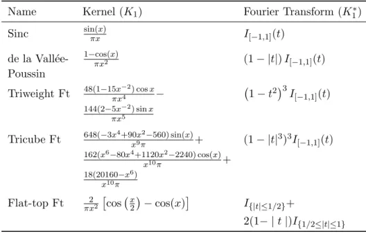
Table 2.1 Kernel functions with their Fourier transforms, where x, t∈R and K1
is continuously extended at zero in every case. . . 15
Table 2.2 Distributions used in the study for signal and noise. Both signal
distri-butions have the same mean and covariance matrix and both error dis-tributions have the same covariance matrix. The bivariate gamma is de-fined here through a Gaussian copula with density is givenfG(g1, g2) =
fG1(g1) φ(Φ−1(F G1(g1))) · fG2(g2) φ(Φ−1(F G2(g2))) ×fZ Φ−1(FG1(g1)),Φ −1(F G2(g2)) for g1, g2>0 depending on parameters,α1,α2,β1,β2>0 and−1< r <1. Fori= 1,2,FGi and fGi denote the distribution and density functions
of a gamma variable with shapeαi and rate βi parameters; Φ−1 and φ
are the quantile function and the density of a standard normal
distribu-tion; andfZ denotes a bivariate normal density with correlation r and
LIST OF FIGURES
Figure 2.1 Plots of kernel functions and their Fourier transforms: Sinc, de la Vall´ ee-Poussin (VP), triweight Fourier transform (triw), tricube Fourier trans-form (triw) and Flat-top Fourier transtrans-form kernels. The kernel function
that oscillates the most is the sinc kernel. . . 16
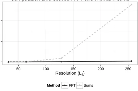
Figure 2.2 Speed comparison of integrating procedures. The Fast Fourier
Trans-form (FFT) is substantially faster than plain Riemann sums for
increas-ingly larger approximation grids. . . 18
Figure 2.3 Contour plots considered for the study. Both distributions have the
same mean and covariance matrix. Observe that the coordinates are correlated in both distributions. The bivariate gamma was generated according to Table2.2. . . 20
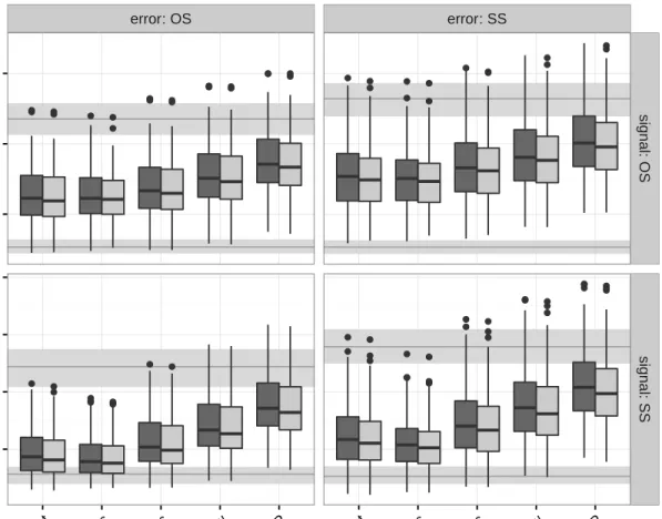
Figure 2.4 Comparison of estimators for different combinations of smoothness when
the noise to signal ratio is equal to 1. Observe that the SS signal and OS noise has the closest performance to the error free case when sinc and flat-top kernels are used. On the other hand, the worst performance overall occurs in the OS signal and SS noise, which is expected. The two background bands represent the three quartiles of the ISE computed for the kernel density estimator of the error free observations (lower band) and the kernel density estimator of the contaminated sample ignoring
the noise (upper band). This plot was generated for m = 2 replicate
Figure 2.5 Comparison of estimators for different noise-to-signal ratio and number of observations per individuals when the empirical characteristic func-tion has been used for approximating the error with SS signal and OS noise. The two background bands represent the three quartiles of the ISE computed for the kernel density estimator of the error free observa-tions (lower band) and the kernel density estimator of the contaminated
sample ignoring the noise (upper band). . . 25
Figure 2.6 The estimation performances based on pre-processing mechanism used
to compute the differences among m = 8 replicates per individual (for
approximating the characteristic function of noise). The left plot con-siders a noise to signal ratio of 1 and the right plot involves a ratio of 2. The two background bands represent the three quartiles of the ISE computed for the kernel density estimator of the error free observations (lower band) and the kernel density estimator of the contaminated sam-ple ignoring the noise (upper band). This plot was generated using the empirical characteristic function to estimate the error (results were sim-ilar the characterstic function of a kernel density estimator, cf. (2.15),
Section 3.1) with OS signal/SS noise data generation. . . 27
Figure 2.7 Perspective plots of the true density and kernel deconvolution density
estimates based on a sample size ofn= 150 varying the kernel function.
The sinc kernel (upper left corner) possess the greatest oscillations . . 29
Figure 3.1 Example of a univariate Fourier integral over grids of several (power of
two) sizes. Specifically, the standard normal density is being recovered using the Fourier inversion formula. Time is in milliseconds. The Fourier integral has been applied five times for every resolution and each dot
Figure 3.2 Example of a bivariate Fourier integral over grids of several (power of two) sizes. Both axis have the same resolution. Specifically, the char-acteristic function of a bivariate normal distribution is being computed.
Time is in seconds (unlike 3.1). The Fourier integral has been applied
five times for every resolution and each dot represents the mean for the
corresponding grid size and method. . . 34
Figure 3.3 Example of fourierin function for univariate function at resolution
64: Recovering a normal density from its characteristic function. See Equation3.3. . . 37
Figure 3.4 Example of fourierin function for univariate function at resolution
128×128: Obtaining the characteristic function of a bivariate normal
distribution from its density. See Equation 3.4. The left plot is the
section of the real part of the characteristic function att1= 0; the right
plot is the section of the characteristic function att2 = 0. . . 40
Figure 4.1 Gamma sample contaminated with Laplacian errors. The error
distri-bution is assumed to be known. This plot shows when the correct dis-tribution, Laplace, was given (long dashed red line) and the incorrect
distribution (normal) was given (dashed green line). . . 45
Figure 4.2 Contaminated sample plus a sample of independent errors. The
charac-teristic function of the error has been approximated with the empirical characteristic function. The error distribution was approximated with the empirical characteristic function. The code that generated this plot can be found in Section4.7. . . 47
Figure 4.3 KDDE on panel data. Code is shown in Section4.7 . . . 48
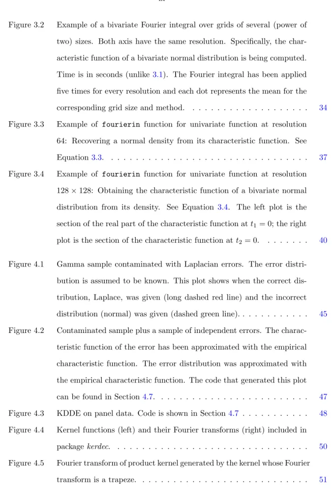
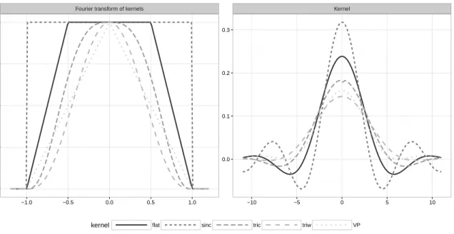
Figure 4.4 Kernel functions (left) and their Fourier transforms (right) included in
package kerdec. . . 50
Figure 4.5 Fourier transform of product kernel generated by the kernel whose Fourier
Figure 4.6 Cross-validation function for KDDE. Code and details can be found in Section4.7. . . 52
ACKNOWLEDGEMENTS
I want to express my deepest gratitude to my advisers, Dr. Alicia Carriquiry, Dr. Daniel Nordman and Dr. Kris De Brabanter. They imparted on me their infinite wisdom, encouraged me, were patient, and gave much of their time so that I could succeed.
I acknowledge my committee members, Dr. Ken Koehler, Dr. Yehua Li and Dr. Lily Wang. Their comments and suggestions on this dissertation were very helpful.
Even the steepest road is easy when you have people on your side. I have always counted on my family and friends - especially on my mother, my sisters and my husband, Lety, Diana, Viry and Mart´ın. My friends in Ames were a valuable source of support.
Every one of my professors at Iowa State University has taught something beyond the
syllabus. My undergraduate and masters advisers, Dr. V´ıctor P´erez-Abreu and Dr. Miguel
Nakamura have mentored me all along the way.
Finally, I want to thank the Department of Statistics and the National Council of Science and Technology of Mexico (CONACyT) for their support.
CHAPTER 1. INTRODUCTION
In many areas of application, like medical sciences, variables of interest are not directly
observable but only through some error contamination. These cases are often referred as
“measurement error problems”.
Kernel deconvolution density estimation (KDDE) is a measurement error problem which consists in estimating the density of a population that is observable only with some error contamination. For sake of clarity, we will use a simple example, suppose that we wish to get an estimate of the distribution of the number of steps taken by a particular population. Portable pedometers do the job, but number of steps may be very different from device to device (even between two devices of the same brand). Thus, the measurement error induced by the device should be taken into account.
Assume for the moment that the distribution of the measurement error is known among the
pedometers used. Then, assume that we have a sampleY1, . . . , Ynthat come from the model
Y =X+, (1.1)
whereX is the (unobservable) distribution of the number of steps andmeasurement error of
the device.
KDDE is a modification of the kernel density estimator (KDE). Recall that the KDE of the sample X1, . . . , Xn from the random variableX is given by
˜ fX(x) = n X i=1 1 nhK x−Xj h , x∈R, (1.2)
where K is a symmetric function that integrates to one, called the kernel function, and h is
˜ f in (1.2) is mathematically equivalent to ˜ fX(x) = 1 2π Z ∞ −∞ exp(−ıxt) ˆφX,n(t)Kf t(ht)dt, x∈R, (1.3) where ˆφX,n(t) = n−1 P
iexp(ıtXi) is the empirical characteristic function of the sample and
Kf t(s) =R exp(ısx)K(x)dxis the Fourier transform of the kernel K.
We cannot use (1.3) with the contaminated sample (even less if the error is not negligible).
The KDDE is a modification of (1.3) that depends directly of the contaminated sample:
ˆ fX(x) = 1 2π Z ∞ −∞ exp(−ıxt) ˆφY,n(t) Kf t(ht) φ(t) dt, x∈R, (1.4) where φ(t) = (2π)−1 R
exp(−ıtx)f(x)dxis the characteristic function of, which has density
f. Therefore, the KDDE and its properties are mostly studied in the frequency domain.
Several challenges arise with the KDDE. We will list next a few of these.
1. Observe in (1.4) that takingK with Fourier transform that is compactly supported would
ensure that the integral exists and it would be easier to compute it. Moreover, convergence rates are easier to find if Kf t has compact support.
2. The integral in (1.4) is hard to obtain due to the oscillating nature of the integrand. It is important to have effective and fast numerical procedures to do it.
3. It is unrealistic most of the times to assume that the error distribution (its characteristic function in particular) is known. In real life it can be approximated by providing an independent sample of errors based on repeated measures. In our pedometer example, we can imagine designing an experiment actually counting the differences in steps to approximate the error distribution. For the latter, every individual could wear several pedometers at the same time, thus there would be repeated observations for the same individual.
4. In the case of having repeated measurements, the observations are not independent. There are several ways to obtain a (contaminated) sample and to obtain observations to approximate the error.
5. Equation 1.4can be generalized to higher dimensions. The literature in that case is not extensive.
6. A challenging problem in KDE is the bandwidth selection. In order to generalize any of the existing methods to KDDE, it is necessary to take it first to the frequency domain. This is not always possible or straightforward.
In this work we approach several of this problems. In particular, in Chapter2we conduct a
numerical investigation of bivariate KDDE to investigate item1 by comparing several kernels
whose Fourier transform has compact support. We pay special attention to a class of kernels referred as “flat-top kernels” (cf. Politis and Romano (1999)). We also study several aspects
of items 3 and 4 in Chapter 2 and compare two nonparametric ways to approximate the
(characteristic function of the) error distribution.
Chapter 3 describes an R package to compute univariate and bivariate continous Fourier
transforms, which is versatile enough to perform integration using any definition of continu-ous Fourier transform and its inverse. The implementation for the regularly spaced grid is an algorithm that uses the so-called Fast Fourier Transform that it is known to reduce drasti-cally the computation time. We actually use the C++ library called Armadillo to speed up computations.
We use the R package described in Chapter 3 to create an R package specialized in fast
computation of KDDE under several scenarios including the ones described in items 3 and 4
for univariate and bivariate samples. This R package also allows the user to approximate the error in a parametric or nonparametric fashion with ease. The bandwidth selection method is based on cross-validation (cf. Youndj´e and Wells (2008)) and it allows the user to visualize the function that had to be minimized to find the bandwidth.
Finally, in Chapter 4 we propose a bandwidth selection which does not require non-trivial
iterative steps and does not require knowledge of the smoothness level of the target distribution
(cf. Delaigle and Gijbels (2004b) and Fan (1991a)). This bandwidth selection method is
CHAPTER 2. A NUMERICAL INVESTIGATION OF BIVARIATE KERNEL DECONVOLUTION WITH PANEL DATA
A paper to be submitted
Guillermo Basulto-Elias, Alicia L. Carriquiry, Kris De Brabanter and Daniel J. Nordman
Abstract
We consider estimation of the density of a multivariate response, that is not observed di-rectly but only through measurements contaminated by additive error. We focus on the realistic sampling case of bivariate panel data (repeated contaminated bivariate measurements on each sample unit) with an unknown error distribution. Several factors can affect the performance of kernel deconvolution density estimators, including the choice of the kernel and the estimation approach of the unknown error distribution. We show that the choice of the kernel function is critically important and that the class of flat-top kernels has advantages over more commonly implemented alternatives. We describe different approaches for density estimation with mul-tivariate panel responses, and investigate their performance through simulation. We examine competing kernel functions and describe a flat-top kernel that has not been used in deconvolu-tion problems. Moreover, we study several nonparametric opdeconvolu-tions for estimating the unknown error distribution. Finally, we also provide guidelines to the numerical implementation of kernel deconvolution in higher sampling dimensions.
2.1 Introduction
A challenge in many areas of application (e.g., medical sciences) is that responses of interest are not observable; instead, responses are measured with error contamination. Such cases are
frequently referred to as “measurement error problems” and arise frequently in applications. An example from nutrition epidemiology is the following. Suppose that we wish to estimate the joint density of the “usual” or long-run average of serum iPTH (intact parathyroid hormone) and 25(OH)D (25-hydroxy vitamin D), both of which are associated with bone health. While daily values for these two substances can be measured reliably, they are noisy estimates of their long-run averages, which are the quantities of interest. Ignoring such measurement error can lead to biased inference. Kernel deconvolution density estimation provides an alternative way to remove measurement error in estimating a target density, without the need for stringent para-metric assumptions. Deconvolution estimation typically involves translation to the frequency domain to approximate the characteristic function of a target variable through the estimated characteristic functions of noisy measurements and errors. Although kernel deconvolution has received much attention for univariate observations, the case of multivariate observations has received less consideration, especially for the more realistic case where little is known or can be immediately assumed about the error distribution and where the observations consist of one or more (correlated) measurements on subjects (i.e., panel data structure). In particular, there has been limited theoretical development for the bivariate panel data case and even less for the multivariate case.
In this paper, we focus on a simulation-based study to explore the performance of deconvo-lution methods, in particular when applied to bivariate panel data. The performance of kernel deconvolution estimation in the multivariate setting depends critically on a combination of factors that have not been well studied. These include the choice of kernel, the way in which panel data are pre-processed, the number of measurements obtained for each sample unit, and the approach to estimating the unknown error distribution. Through simulation, we study the impact of these potentially important factors in order to better understand the practical issues associated with implementation of kernel deconvolution and to inform possible future theoretical developments in this area.
In addressing bivariate kernel deconvolution, we consider five candidate kernel functions for which the Fourier transform has bounded support, include the sinc kernel (a popular choice in the univariate case) and a trapezoidal flat-top (where the latter is novel in deconvolution
problems). Additionally, we compare different approximations to the (unknown) characteristic function of the errors with panel data. Such approximations involve choices on how to incor-porate replicate measurements and combine these with either a direct empirical estimator or an indirect kernel density-based estimator of the characteristic function of the error. Perhaps surprisingly, our findings suggest that in contrast to some claims in the univariate setting, the way in which panel data are processed (i.e., differenced to estimate the error distribution) has little impact, and that kernels commonly used with univariate measurements do not perform as well as other kernels (e.g., ”flat top”) studied here for the multivariate case. Further, ker-nel deconvolution estimators for multivariate responses pose more computational challenges, in particular for numerical integration. To overcome the computational challenges, we use an algo-rithm based on a Fast Fourier Transform (FFT) that improves efficiency without compromising accuracy .
We end this section with a brief review of the literature. An extensive discussion of the univariate deconvolution problem can be found in Meister (2009). For the multivariate setting, asymptotic convergence properties when the error distribution is assumed to be known can be found in Masry (1991, 1993a,b). The selection of a single bandwidth parameter (diagonal
band-width matrix with equal diagonal entries) using cross-validation was proposed by Youndj´e and
Wells (2008) while Comte and Lacour (2013) who also focused diagonal bandwidth matrices, proposed estimating its diagonal elements as the minimum of an empirical approximation to the asymptotic integrated mean squared error. Johannes (2009) and Comte and Lacour (2011) considered the situation where the error distribution is unknown, but a sample of pure errors is available. None of these papers considered multivariate panel data (i.e., repeated multivariate measurements on each subject, contaminated with error). In the univariate panel data setting, with unknown error distribution, several approaches have been proposed for estimating the characteristic function of the error. Delaigle and Meister (2008) suggested using all possible measurement differences available for each individual with deconvolution applied to the mea-surement averages per subject. Stirnemann et al. (2012b) and Comte et al. (2014) proposed taking simple pairwise differences of the replicate measurements to approximate the character-istic function of the error; only the first noisy measurement on each subject is then used in the
deconvolution steps that follow. Ridge terms or truncation, as in Neumann and H¨ossjer (1997), are typically applied to control the estimated characteristic function of errors for small values. For the vast majority of the literature discussing deconvolution with univariate panel data, the most frequently chosen kernel is the sinc kernel because it has been shown to have good theoretical properties (e.g., its Fourier transform is flat around zero as suggested by Devroye (1989)) and because its form permits applying the FFT for numerical integration.
This paper is organized as follows. Section 2.2 describes the general density estimation
problem and how it can be approached with kernel methods, with special attention to the
panel data case introduced in Section 2.2.2. In Section 2.3, we outline several potentially
important attributes of the deconvolution method that may impact performance. In particular,
Section 2.3.1 discusses how to approximate the characteristic function of errors from a panel
data structure, and Section 2.3.2describes candidate kernel functions. Section 2.3.3 provides
numerical integration tools required for bivariate kernel density deconvolution. In Section 2.4
we present the design of a large simulation study and discuss the numerical results. Finally, conclusions are presented in Section 2.5.
2.2 Problem description
We first outline the estimation method for multivariate kernel density deconvolution in general. Section2.2.1introduces some initial background in the context of a simplified version of
kernel deconvolution density estimation in the multivariate setting. Section2.2.2then discusses
the case of multivariate panel data and some related estimation issues that arise in this situation.
For illustration purposes, we focus on the case of bivariate measurements X ∈ Rd, d = 2,
although generalizations to any dimensiondof the observation vector are possible.
2.2.1 A simplified estimation framework
Suppose that we are interested in estimating the distribution of a two-dimensional random
variable X that cannot be directly observed. Instead we observe X convoluted with random
noise, say, Y = X +, where ∈ R2 is the random noise vector. The standard
measurements
Yi =Xi+i, (2.1)
fori= 1, . . . , n. In (2.1), the collection{Xi}ni=1 is independent and identically distributed (iid) and so is the variable set {i}ni=1. Furthermore, for each measurement Yi, the responseXi of
interest is assumed to be independent of the error i.
We require some notation before introducing the deconvolution formulas. LetφY(·) denote
the characteristic function (CF) of the random sampleY1, . . . ,Yn, and let ˆφY,n(·) denote the
empirical CF. That is, for anyt∈R2,
φY(t) =E eıt·Y1 and ˆφY,n(t) = 1 n n X j=1 eıt·Yj,
where the dot product · above represents the usual inner product in R2 and ı =
√
−1. For a
real-valued functiong:R2 →R, denote its Fourier transform byg∗, where
g∗(t) =
Z
eıt·xg(x)dx. (2.2)
When g is a (multivariate) density function, theng∗ represents its CF.
By the independence of Xi andi in (2.1), the CF φX(·) of the uncontaminated
measure-ments X can be obtained from that ofφY(·), the CF of the observed measurements, as
φX(t) =
φY(t)
φ(t)
, t∈R2,
whenever the CF of the errors φ(·), is non-zero (i.e., t∈ R2 with φ(t) 6= 0). Consequently,
by applying the Fourier inversion theorem, we can compute the density ofX atx∈R2 as
fX(x) = 1 (2π)2 Z e−ıt·xφY (t) φ(t) dt, (2.3)
which is the distribution of the uncontaminated response X. Because φY is typically
un-known, we may replace it with its empirical version, ˆφY,n, but the resulting function in (2.3)
might not be integrable. However, by substituting a smoothed estimator version instead, say ˆ
φY,n(t)K∗(Bnt), we obtain a valid (kernel) estimator of the density of X as
ˆ fX,n(x) = 1 (2π)2 Z e−ıt·xφˆY,n(t) K∗(Bnt) φ(t) dt, x∈R2. (2.4)
HereK∗ denotes the Fourier transform of a smoothing kernelKandBndenotes a 2×2 (positive
definite) bandwidth matrix.
Note that (2.4) assumes that the CF of the underlying error terms,φ, is known. Under the
general data model (2.1), it is frequently assumed that either the error distribution is known
or that there exists a sample of pure errors, obtained independently of Y1, . . . ,Yn, that can
be used to estimate the error CF (see Johannes (2009) and Comte and Lacour (2011)). These assumptions are often unrealistic in many applications. Therefore, in this paper we will not
make such assumptions when describing the estimation with panel data in Section 2.2.2.
2.2.2 Kernel deconvolution estimation with panel data
We now discuss kernel density deconvolution estimation for bivariate panel data. For such data, an additive noise model is given by
Yij =Xi+ij, (2.5)
for i = 1, . . . , n and j = 1, . . . , m. Here Yij represents the d = 2 observations for the
i-th individual on i-the j-th measurement occasion. As in model (2.1), the iid uncontaminated
response variables{Xi}ni=1 are independent of the iid errors{ij :i= 1, . . . , n;j= 1. . . , m}.
For simplicity, and without loss of generality, we assume that the numbermof observations
is the same for every sample unit (individual). Note that while sample units are assumed to be
independent, the components among thed-dimensional measurements for each unit are typically
not independent, and the replicate measurements obtained on each unit are also correlated. We wish to estimate the joint densityfX of the uncontaminated variables{Xi}ni=1. Under a
panel data structure, the standard deconvolution density estimator (2.4) needs to be modified
to account for the dependence among replicate measurements on each sample unit. That
is, measurements made on the same subject are no longer independent, as was the case in Section 2.1 (i.e., instead two measurementsYij and Yi0j0 are independent only ifi6=i0).
As in the univariate panel data setting, there are several ways to account for the panel data structure when using the estimator (2.4) of the densityfX. Comte et al. (2014) use only the first
However, this approach ignores the other m−1 measurements available for each subject and therefore may entail some information loss. Instead, we propose making use of all observations obtained on each subject to compute an average measurement for individual; we then
re-formulate the deconvolution estimator to be based on the CF of the averages, say φY¯, rather
than on the CF of individual responses φY in (2.4). That is, we first average observations in
(2.5) per individual,
¯
Yi·=Xi+ ¯i·, i= 1, . . . , n. (2.6)
When the response variable is the average of m replicate measurements, the error term ¯i·
in (2.6) represents an average of m iid error variables with CF given by φ¯(t) = [φ(t/m)]m
in terms of the CF φ of an original (i.e., single) error term in the panel data model (2.5).
Therefore, instead using the kernel density deconvolution estimator (2.4), we use a modified
estimator given by ˆ fX,n(x) = 1 (2π)2 Z e−ıt·xφˆY¯,n(t) K∗(Bnt) φ¯(t) dt (2.7) = 1 (2π)2 Z e−ıt·xφˆY¯,n(t) K∗(Bnt) [φ(t/m)]m dt,
for x ∈ R2 based on the CF of error averages, [φ
(t/m)]m and the empirical CF of subject
averages is {Y¯i}ni=1, ˆφY¯,n(t) =n−1
Pn
j=1eıt ·Y¯j
,t∈R2.
However, there are several issues that require examination when implementing an estimator
of the form (2.7) with panel data. These can impact the performance of the kernel deconvolution
estimator ˆfX,n, which we numerically investigate in Section 4. Firstly, the error distribution is
typically unknown so that the associated CFφ in (2.7) needs to be estimated. By exploiting
the repeated measurement in the panel data structure, we can construct at least two different estimators, both of which are based on differences between measurements within subjects. We
elaborate on this issue in Section 2.3. Potential formulations for constructing differences
be-tween measurements in panel data are also outlined in that section. A second issue that arises is that the deconvolution formula (2.7) requires specification of a multivariate kernel function
and the bandwidth matrix for that kernel. Section2.3.2discusses several types of kernels that
may be considered, including “flat-top” kernels that have been successfully used for spectral density estimation but that have not been applied in deconvolution problems (cf. Politis and
Romano (1995), Politis (2003b), Politis and Romano (1999)). Finally, the deconvolution esti-mator includes integrals that are often numerically approximated; in contrast to the univariate data, the multivariate setting introduces further challenges for the evaluation of a density es-timator ˆfX,n(x) at vector points x∈R2. In Section 2.3.3, we describe some numerical recipes that greatly improve computational efficiency in the multivariate deconvolution setting.
2.3 Challenges in deconvolution estimation with panel data
2.3.1 Estimation of the error distribution
Assume for now that the number m of observations for each individual is even for the
panel data (2.5). In the univariate setting, Comte et al. (2014) proposed constructing pairwise
differences between repeated measurements (within individuals) as
Yi,2l−1−Yi,2l=i,2l−1−i,2l, (2.8)
fori= 1, . . . , n and l= 1, . . . , m/2. The reason for formulating differences within individuals is that the measurement differences correspond to differences in error terms (i.e., common
unobserved variablesXi drop out). Each measurement is used only once to create a difference
in (2.8), and therefore the nm/2 differences across all individuals are iid. Another possibility is to consider all possible within-individual differences, as in Delaigle and Meister (2008); that is
Yi,j −Yi,j0 =i,j−i,j0, (2.9)
fori= 1, . . . , nandj < j0. This approach results in a higher number of measurement differences
(i.e., nm(m−1)/2 differences) which, though identically distributed, are not independent.
Finally, we might also consider an intermediate method, which leads to an intermediate sized
collection of measurement differences, with a weaker dependence structure relative to (2.9). In
this approach, the last m−1 measurements for each sample unit are deviated from the first
one as follows:
fori= 1, . . . , n and j = 2,3, . . . , m. In this case, there aren(m−1) measurement differences which are not independent. In contrast to (2.8), the differencing strategies (2.9) and (2.10) do not require an even number of observations per individual. The simulation experiments in
Section 2.4 compare the performance of deconvolution estimators based on these three types
of measurement differences.
Regardless of the chosen approach, the processed data consist of a collection of differenced measurements or error differences, say δ1, . . . ,δk, where the number of differences k depends
on the differencing approach (2.8)-(2.10). We propose a methodology to estimate the error CF
φ in (2.7) with these differences. By the iid property of individual error terms, observe that,
fort∈R2 and j6=j0, the CF φδ of a within individual measurement difference is given by
φδ(t) =φi,j−i,j0(t) =φi,j(t)φi,j0(−t) =φ(t)φ(−t) =|φ(t)|
2. (2.11)
If we assume that the distribution of the panel data errors is symmetric and its CF is never zero, then
φ(t) =
p
φδ(t) (2.12)
holds whenφ is real-valued (by symmetry) and also positive (byφ(0) = 1 and by the
assump-tion that φ is never zero). Thus, under the multivariate panel data structure, an estimator
for the CF of an error term,φ, is given by
ˆ φ(t) = r < ˆ φδ(t) , t∈R 2, (2.13)
where <(.) denotes the real part of a complex number and ˆφδ(t) = k−1Pkj=1 exp (ıt·δj),
t∈R2, is the empirical CF of the measurement differences{δ
j}kj=1.
Note that the estimator (2.13) of the (single) error term does not require stringent assump-tions on the distribution of the errors. To our knowledge, empirical CFs seem to be the main nonparametric approach for estimating such error CFs in the deconvolution literature (albeit often in the non-panel data setting where an independent sample of pure errors is assumed to
be available). In the simulations of Section 2.4, we also consider an alternative approach for
estimating the error CF, for comparison to the empirical CF (2.13) of differences. This
estimator for the distribution of the differences; a Fourier transform of this density then pro-vides an estimator ˆφδ of the CFφδ. Instead of the empirical CF of differences, this estimator
ˆ
φδ can then be substituted in (2.13) to approximate the error term CF φ, which generally
produces a smoother version of the empirical CF based on differences. Suppose a kernel density
estimator is used to approximate the density ofδ, using a (bivariate) kernelL and bandwidth
matrix Σ. The corresponding CF of the density estimator is then given by ˆ φδ(t) = 1 M M X j=1 exp (ıt·δj)L∗ Σ1/2t , t∈R2. (2.14)
In particular, ifLis the product kernel (see Section2.3.2) generated by the normal distribution, we have ˆ φδ(t) = 1 M M X j=1 exp ıt·δj− 1 2t 0 Σt , t∈R2. (2.15)
We choose a normal kernel above because its Fourier transform (2.15) has an efficient, closed
expression. Another possibility, not considered here, would be to use the CF of a normal
mixture with a data-driven number of components. In Section 2.4, we specify how we select
the bandwidth matrix Σ.
Ultimately, an estimated CF ˆφof the error (or an estimator ˆφ¯) appears in the denominator
of the deconvolution formula (2.7). This means that numerical approximations or estimates of
this CF can potentially lead to instabilities for small values of the CF. Several authors have proposed ways to avoid computational issues when using an estimated error CF in the denomi-nator of the deconvolution estimator. For example, Meister (2009) describes two regularization methods: either use a ridge parameter or truncate the denominator in the deconvolution
for-mula when the value of the estimated CF is very small. In our sifor-mulations (see Section 2.4),
we truncate the integrand when the denominator in (2.7) has small values, as in Neumann and
H¨ossjer (1997). Namely, the term 1/φ¯(t) = 1/[φ(t/m)]m is approximated by
1 ˆ
φ¯(t)
I{|φ¯ˆ(t)|> bn,m}, (2.16)
for ˆφ¯(t) = [ ˆφ(t/m)]m based on the estimated error CF ˆφ (i.e., using one of the approaches
described above) and forbn,m = 1/
√
k based on the numberkof differences used to determine
ˆ
2.3.2 Choice of kernel function
In standard kernel density estimation, it is common to construct multivariate kernel func-tions starting with univariate kernels. The simplest approach is to define a multivariate kernel as a product of univariate kernels
K(x) =K1(x1)K1(x2), x= (x1, x2)∈R2, (2.17)
where K1 is a univariate kernel function. Such multivariate kernels (2.17) are called product
kernels and their corresponding Fourier transform is given by
K∗(t) =K1∗(t1)K1∗(t2), t= (t1, t2)∈R2. (2.18)
Another alternative, not pursued here, is the family of radial-symmetric kernels (cf. Wand and Jones (1995)).
Computation of the deconvolution kernel density estimator (2.4) or (2.7) involves integration over the domainR2 (i.e., for bivariate data). If a bivariate kernelK is chosen in such way that its Fourier transformK∗ has bounded support, then the integral in (2.7) is restricted to a finite
region. In what follows, we choose univariate kernels K1 = K2 that have Fourier transforms
with support on an finite interval, say [−1,1]. Then, without loss of generality, the resulting bivariate product kernel has Fourier transformK∗ supported on [−1,1]×[−1,1]. Because this bounded-support property simplifies integration and is also associated with kernels that have good properties, this type of kernel function is commonly used in deconvolution applications. Table2.1displays various univariate kernel functionsK1and their respective Fourier transforms K1∗ for application in (2.18) and then (2.7).
Among univariate kernels K1 with a Fourier transform with bounded support, the most
common is the sinc kernel, whose Fourier transform K1∗ corresponds to a simple indicator
function. The sinc kernel has well-known theoretical advantages (see below), but is not non-negative. Consequently, density estimates based on the sinc kernel tend to exhibit wiggly behavior at the tails, with an unattractive appearance; this behavior is illustrated wth numerical examples in Section 2.4.
As pointed out by Devroye (1989), kernels K1 which perform well in estimation can often
Table 2.1 Kernel functions with their Fourier transforms, where x, t∈R and K1 is continu-ously extended at zero in every case.
Name Kernel (K1) Fourier Transform (K1∗)
Sinc sin(πxx) I[−1,1](t)
de la Vall´ee- 1−πxcos(2x) (1− |t|)I[−1,1](t)
Poussin Triweight Ft 48(1−15πxx−42) cosx− 1−t2 3 I[−1,1](t) 144(2−5x−2) sinx πx5 Tricube Ft 648(−3x4+90xx9π2−560) sin(x)+ (1− |t|3)3I[−1,1](t) 162(x6−80x4+1120x2−2240) cos(x) x10π + 18(20160−x6) x10π Flat-top Ft πx22 cos x2−cos(x) I{|t|≤1/2}+ 2(1− |t|)I{1/2≤|t|≤1}
has this feature, but other kernels are often adopted because they produce smoother estimates
of the target density. An alternative to the sinc kernel is the de la Vall´ee Poussin kernel (VP
kernel), defined in Table2.1. This kernel is actually a probability density (i.e., is nonnegative),
but its Fourier transform is sharp around zero and the numerical findings in Section2.4suggest
that this kernel exhibits poor performance for bivariate deconvolution density estimation. Between the sinc and VP kernels, there are other kernel functions whose Fourier transforms are flat around zero to varying degrees. We consider three of them (triweight, tricube,
trape-zoidal flat-top), described in Table 2.1. Figure 2.1displays all the kernels we have mentioned
and their Fourier transforms. The kernel with Fourier transform proportional to the triweight kernel was used by Delaigle and Gijbels (2004b,a), and resembles the kernel whose Fourier
trans-form is proportional to the tricube kernel in Table2.1. The flat-top kernel has been seemingly
unknown in the deconvolution literature but has established properties in density estimation for time series (cf. Politis (2003b)). Section2.4demonstrates that the flat-top kernel produces density estimates with attractive shape properties while maintaining good (integrated squared error) performance relative to the other commonly used kernels for deconvolution estimation.
Fourier transform of kernels Kernel 0.00 0.25 0.50 0.75 1.00 0.0 0.1 0.2 0.3 −1.0 −0.5 0.0 0.5 1.0 −10 −5 0 5 10
kernel flat sinc tric triw VP
Figure 2.1 Plots of kernel functions and their Fourier transforms: Sinc, de la Vall´ee-Poussin
(VP), triweight Fourier transform (triw), tricube Fourier transform (triw) and Flat-top Fourier transform kernels. The kernel function that oscillates the most is the sinc kernel.
2.3.3 Numerical Implementation
The deconvolution kernel density estimator ˆfX,n in (2.7) requires the computation of an
integral that does not have a closed expression, and the oscillatory nature of the integrand introduces challenges for numerical approximations. We provide numerical integration recipes to address this practical issue. General-purpose software and algorithms for evaluating inte-grals in multiple dimensions do exist (mostly Monte Carlo methods); an example is the package called CUBA, described in Hahn (2005). However, when applying such methods to compute the estimator ˆfX,n(x) at different values x ∈ R2, the exponential term in the integrand in
(2.7) is evaluated repeatedly for the same x values, which is time-consuming and
computa-tionally wasteful. Therefore, we propose approximating the integrals in (2.4) using faster and
One simple approximation to the integral (2.7) is based on Riemann sums as ˆ fX,n(x) = 1 (2π)2 Z [−1,1]2 e−ıt·xφˆY¯,n(t)K ∗(B nt) φ¯(t) dt (2.19) ≈ ∆ (2π)2 X t∈G e−ıt·xφˆY¯,n(t) K∗(Bnt) φ¯(t) ,
where G denotes a regular grid on [−1,1]2 of L
1·L2 (Li points in the i-th coordinate) and
∆ denotes the area between grid points. Note that the integration limits are [−1,1]2 rather
than R2 when we focus on kernel functions with Fourier transforms supported on [−1,1]2.
(Furthermore, in practice, one would estimate 1/φ¯(·) as described in Section 3.1.)
In application, we also need to evaluate the density estimator ˆfX,n(·) over a grid of points
ofX so that probability estimates can be obtained by numerically integrating ˆfX,n(·). This is
a different matter than the problem of computing ˆfX,n(·) at a single point x, see Comte and
Lacour (2010). For that purpose, we carry out density estimation ˆfX,n(x) on a regular grid of
pointsx, say on [c1, d1]×[c2, d2] with L3·L4 points; here c1, d1, c2, d2 denote the bounds of a rectangular region for computing density estimators, selected by the user.
We considered two approaches for computing the Riemann sums in (2.19). The first
ap-proach computes all quantities in (2.19) which do not depend on x (requiring evaluation
only on the subgrid G ⊂ [−1,1]2) and then evaluates exponential terms at x-points on the
[c1, d1]×[c2, d2] to determine the Riemann sums. Another alternative is to use the Fast Fourier
Transform (FFT) to compute the approximating sums in (2.19). We used the FFT method
developed in Inverarity (2002a), which is the generalization to the multivariate case of Bailey and Swarztrauber (1994).
The FFT forcesL1 =L3andL2 =L4, which is a restriction compared to the plain Riemann
sum method. However, the FFT approach is much faster, as can be seen in Figure2.2. Figure
2.2compares the time required to obtain density estimates on a grid (using simulated panel data
described in Section2.4) based on both the FFT and plain Riemann sum approaches. (For the
sake of simplicity, to produce the Figure2.2, we considered the same resolution for evaluating
both methods, that is, L1 = L2 = L3 = L4). Note that both approaches have the same
numerical accuracy as each computes the same Riemann approximation (2.19) to the integral.
● ● ● ● 0 2000 4000 50 100 150 200 250 Resolution (L1) seconds Method ● FFT Sums
Computation time between FFT and Riemann sums
Figure 2.2 Speed comparison of integrating procedures. The Fast Fourier Transform (FFT) is
substantially faster than plain Riemann sums for increasingly larger approximation grids.
[−1,1]2, creating larger computational demands where the FFT has speed advantages. Hence,
we recommend the use of the FFT based approach in practice to approximate integrals for bivariate deconvolution estimators. In what follows, we implemented the FFT approximation to carry out all calculations in the simulation studies to follow.
We have also developed a software package called fourierin, made available in R, for
computing multivariate deconvolution estimators on a grid through the FFT-based numerical approximations of the required integrations; see Basulto-Elias et al. (2016).
2.4 Simulation study
2.4.1 Design of the simulation study
Next, we examine several aspects which impact the performance of bivariate kernel deconvo-lution through simulation. We begin by describing distributions for data generation and for the
underlying target density. Fan (1991b) characterizes distributions according to thesmoothness
esti-mate the target density of the underlying signal variable. Formally, a (possibly multivariate)
random variable X is said to beordinary smooth (OS) if there exist positive constants β, d0
and d1 such that
d0|t|−β ≤ |φX(t)| ≤d1|t|−β, as|t| → ∞,
and it is said to be supersmooth (SS) if there exist positive constants β,δ, γ, d0 and d1 such that d0|t|−βexp −γ|t|δ≤ |φ X(t)| ≤d1|t|−βexp −γ|t|δ, as|t| → ∞,
where | · | is the Euclidean norm. Unlike OS variables, SS random variables have densities
which are infinitely differentiable. In the univariate case, examples of OS random variables include those with the gamma distribution and the Laplace distribution while examples of SS distributions include Gaussian and Cauchy densities. To understand the impact of distribution smoothness on deconvolution estimators here, note that the empirical characteristic function
(CF) of the contaminated samples appears in the numerator of (2.4), while the CF of the error
appears in the denominator. This same ratio of CFs also arises in asymptotic expansions for mean squared error of deconvolution density estimators. As a consequence, supersmooth error terms then lead to slower convergence rates in density estimation, because they introduce an additional exponential term into such expansions.
For the simulation, we then considered the following design factors related to data-generating process (item 1 below), number of available replicates (item 2) and estimation implementation (items 3-5) in order to examine their impact on the deconvolution estimators with panel data. 1. We considered four combinations of OS/SS signal/error distributions along with three
varying levels of noise to signal variance ratios (0.2,1,2), as described further below.
2. We assumed either m = 2 or m = 8 replicated measurements for each individual in a
panel data model (2.5) withn= 150 individuals.
3. We compared the five kernel functions described in Table2.1.
4. We implemented the three procedures described Section 2.3.1for creating “error
Table 2.2 Distributions used in the study for signal and noise. Both signal distri-butions have the same mean and covariance matrix and both error
dis-tributions have the same covariance matrix. The bivariate gamma is
de-fined here through a Gaussian copula with density is given fG(g1, g2) =
fG1(g1) φ(Φ−1(F G1(g1))) · fG2(g2) φ(Φ−1(F G2(g2))) ×fZ Φ−1(FG1(g1)),Φ −1(F G2(g2)) for g1, g2 > 0 depending on parameters,α1,α2,β1,β2>0 and−1< r <1. Fori= 1,2,FGi and
fGi denote the distribution and density functions of a gamma variable with shape
αi and rate βi parameters; Φ−1 and φ are the quantile function and the density
of a standard normal distribution; and fZ denotes a bivariate normal density with
correlation r and standard normal marginal distributions.
Type Distribution
OS signal Bivariate gamma with mean (10,2) and cov.
5 −1.75
−1.75 2
, whose marginals are gamma with shape parameters 20 and 2 and rate paremeters 2 and 1, respectively.
SS signal Bivariate normal with mean (10,2) and cov.
5 −1.75
−1.75 2
.
OS noise Laplace with mean (0,0) and correl. matrix
1 .5534
.5534 1
.
SS noise Normal with mean (0,0) and correl. matrix
1 .5534 .5534 1 . −2.5 0.0 2.5 5.0 7.5 5 10 15 x1 x2
Bivariate normal (SS signal)
−2.5 0.0 2.5 5.0 7.5 5 10 15 x1 x2
Bivariate gamma (OS signal)
Figure 2.3 Contour plots considered for the study. Both distributions have the same mean
and covariance matrix. Observe that the coordinates are correlated in both
5. We implemented two different approximations to the characteristic function based on error differences: either the empirical CF from differences or the Fourier transform of a kernel density estimator applied to differences, as described in Section 2.3.1.
Hence, we include four combinations of ordinary smooth (OS) and supersmooth (SS) distribu-tions across the signal and the noise (item 1), where random errors are generated either from a bivariate normal distribution (SS error) or a bivariate Laplace distribution with the same covariance matrix (OS error), and where signal random variable is generated from either a bivariate normal distribution (SS signal) or from a bivariate gamma distribution (OS signal).
Table2.2shows two signal distributions (OS/SS) have the same mean and variance properties,
while Figure2.3 shows the contour plot of the distribution of the signal. With regard to noise
to signal ratios (item 1), we considered three ratios 0.2,1,2 to represent low to high levels of error. These ratios were component-wise fixed for the marginal distributions; that is, for a noise to signal ratio of 0.2, the first components of the error and signal have a variance ratio of 0.2, and the same holds for the second component. For the kernel density-based approximation
to the CF of the errors (item 5), we used a normal kernel, as described in Section2.3.1, with a
diagonal bandwidth matrix obtained with a plug-in method computed using the R package ks
(see Duong et al. (2007)).
In computing the deconvolution estimators, we used a grid of 64×64 points to approximate
the integral in (2.7) via fast Fourier transform (as described in Section 2.3.3) and also for
evaluating the density of the signal variable. There was no significant improvement in precision for larger grid sizes. Moreover, the region for the density estimation was fixed at [3,18]×[−2,9], which contains at least 99% of the mass of both OS/SS signal distributions considered (see
Figure 2.3). For each simulated panel data set and deconvolution estimator, we evaluated the
corresponding the integrated squared error (ISE) through the approximation
Z h ˆ fX,n(x)−fX(x) i2 dx≈∆X ij h ˆ fX,n(xij)−fX(xij) i2 ,
where ∆ = τ1τ2/642 is the area of every grid rectangle for τ1 = 11 and τ2 = 15, and xij =
were computed over 200 simulation runs per data-generating process, and are summized in figures to follow (e.g., boxplots).
Finally, we make some comments about bandwidth effects, which we sought to control in or-der to quantify the impact of the factors mentioned above (e.g., type of kernel) for multivariate panel data with unknown errors. Bandwidth selection is a challenging problem in kernel de-convolution with a rich literature for univariate data (see Delaigle and Gijbels (2004b)), but far less is known for multivariate data. To minimize the compounding effect of bandwidth choice, we used the diagonal bandwidth matrix for minimizing the integrated squared error (ISE) for deconvolution kernel density estimators based on known (not estimated) measurement and er-ror CFs. That is, we employ a diagonal bandwidth matrix for each kernel by choosing the best approximate bandwidths for these kernels, but we do not assume that the distributions of the errors or the signal are known in the simulation study.
2.4.2 Simulation results
To present the simulation findings, we mention two reference estimators that we adopted in order to help frame the performances of bivariate deconvolution estimators. These reference estimators are obtained from kernel density estimators (without deconvolution) applied to samples defined by either (2.20) or (2.21) as
X1, . . . ,Xn (Error free) (2.20)
¯
Y1·, . . . ,Y¯n· (Contaminated) (2.21)
using the normal kernel and a plug-in bandwidth matrix (from the R package decon). The
first estimation reference, which serves as a type of lower bound in estimation error (
error-free in plots), is the usual bivariate kernel density estimation applied to the sample {Xi}ni=1
without measurement error, which is unobservable in practice. However, one wishes for the ISE of a deconvolution estimator to be close to the ISE of this reference estimator, which can be generally expected to exhibit better performance than deconvolution counterparts based on
data with true errors in variables. The second reference estimator (contaminated in plots) aims
density estimator applied to the measurement averages per individual{Y¯i}ni=1from (2.6). Note that this reference estimatorignoresmeasurement errors inherent to the averages (2.21). Hence, as the purpose of kernel deconvolution is precisely to account for measurement error, one would like for devoncolution density estimators to have smaller ISEs than this reference.
Figure 2.4 provides a comparison of average ISEs for the different kernel choices in
decon-volution estimation with panel data across the four distributional cases of ordinary smooth/
supersmooth (OS/SS) signal and OS/SS noise (withm= 2 replicates per individual and noise
to signal ratio of one). The figure also considers the type of estimation for the error/noise characteristic function, based on either the empirical characteristic function (ecf) or the char-acterstic function of a kernel density estimator (kde) (formed by differences between measure-ment replicates). As expected, SS error distributions tend to induce larger ISEs on average compared to OS errors and the smoothness of the underlying signal also impacts performance of deconvolution estimators. However, the effect of the kernel choice is qualitatively similar
in Figure 2.4, where the sinc kernel has the best performance closely followed by the flat-top
kernel in every scenario. The estimaton approach for the error charactersitic function (i.e., ecf or kde) typically resulted in only small differences in performance, with a small but consistent edge for the kde-based method. Note also that deconvolution estimators often substantially
improve upon the contaminated reference in Figure 2.4 (upper horizontal bar) which ignores
measurment error in density estimation, but as expected perform worse than the estimation reference when no measurment error is present (lower horizontal bar).
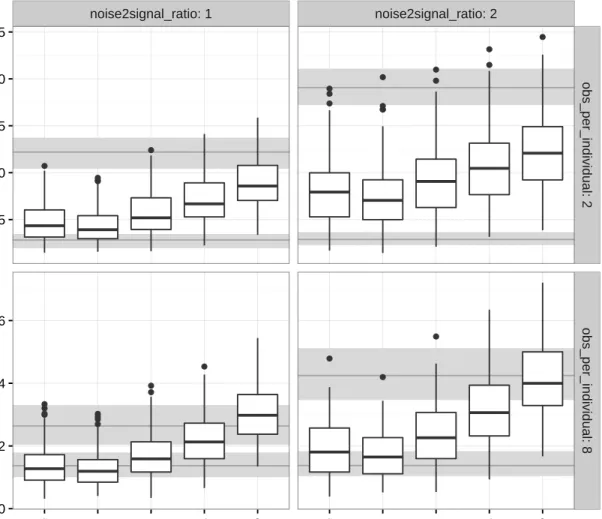
A similar pattern emerges in Figure 2.5, which considers the effect of both differing noise
to signal ratios and varying amounts of replication (m= 2,8). From the figure, the expected
estimation error (ISE) decreases when the number of replicates grows fromm= 2 tom= 8, and
errors also increase as the noise to signal ratio increases. However, regardless of these factors, the results are again qualitatively similar across types of kernel choices, and the flat-top and sinc kernels emerge as the best performers. In particular, with higher numbers of replicates and low noise to signal ratios (ideal inference situations with panel data), deconvolution estimators based on flat-top and sinc kernels achieve error rates similar to the oracle type reference of kernel estimation based on observations with no measurement error (lower horizontal bar in
error: OS error: SS ● ● ● ● ● ● ● ● ● ● ● ● ● ● ● ● ● ● ● ● ● ● ● ● ● ● ● ● ● ● ● ● ● ● ● ● ● ● ● ● ● ● ● ● ● ● ● ● ● ● ● ● ● ● ● ● ● ● ● ● ● ● ● ● ● ● ● ● ● ● ● 0.005 0.010 0.015 0.0025 0.0050 0.0075 0.0100 signal: OS signal: SS
flat sinc tric triw VP flat sinc tric triw VP
ISE
Error approximation: ecf kde
Figure 2.4 Comparison of estimators for different combinations of smoothness when the noise
to signal ratio is equal to 1. Observe that the SS signal and OS noise has the closest performance to the error free case when sinc and flat-top kernels are used. On the other hand, the worst performance overall occurs in the OS signal and SS noise, which is expected. The two background bands represent the three quartiles of the ISE computed for the kernel density estimator of the error free observations (lower band) and the kernel density estimator of the contaminated sample ignoring
the noise (upper band). This plot was generated form= 2 replicate observations
noise2signal_ratio: 1 noise2signal_ratio: 2 ● ● ● ● ● ● ● ● ● ● ● ● ● ● ● ● ● ● ● ● ● ● ● ● ● ● ● ● ● ● ● 0.0025 0.0050 0.0075 0.0100 0.0125 0.000 0.002 0.004 0.006 obs_per_individual: 2 obs_per_individual: 8
flat sinc tric triw VP flat sinc tric triw VP
ISE
Figure 2.5 Comparison of estimators for different noise-to-signal ratio and number of
observa-tions per individuals when the empirical characteristic function has been used for approximating the error with SS signal and OS noise. The two background bands represent the three quartiles of the ISE computed for the kernel density estimator of the error free observations (lower band) and the kernel density estimator of the contaminated sample ignoring the noise (upper band).
Figure 2.5), which also supports these kernel choices. Again, ignoring measurement error (simply averaging observations over replicates and applying ordinary kernel density estimation techniques) is seen to create larger estimaton errors compared to deconvolution approaches (upper horizontal bar in Figure2.5), as particularly evident for small replicationm= 2.
We mentioned in Section2.3.1that there are several strategies to obtain differences to
ap-proximate the characteristic function of the error. Specifically, taking all the possible difference of observations for the same individual (cf. (2.9)), which leads to many correlated observations of differences of errors; taking differences of paired columns, obtaining fewer but independent
error differences (cf. (2.10)), and everything minus the first repetition for individual, which
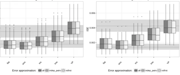
is an compromise between number of observations and independence (cf. (2.8)). Figure 2.6
compares performances for deconvolution estimators based on this type of pre-processing used for creating error differences from replicate measurements in the panel data structure. This
illustration considers the m= 8 replicate case (as the type of differencing is not an issue with
m = 2 replications). Essentially from this figure, the type of pre-processing has surprisingly
little effect, which remains true as the noise ratio increases.
2.4.3 Kernel choices
Among the previous simulation findings, the choice of kernel emerges as the single most in-fluential factor for the performance of deconvolution estimators to be considered in application. While the sinc kernel (sinc) has been widely used in the literature for univariate deconvolu-tion and also exhibited consistently good performance in our simuladeconvolu-tions, the flat-top kernel emerged with a performance similar to the sinc kernel in terms of average ISE. In fact, in many simulation cases, the mean ISEs of deconvolution estimators from both sinc and flat-top kernels were close to the reference estimator based on error free samples. However, an addi-tional potential advantage of the flat-top kernel is that this tends to produce density estimators without the “wiggly” (and sometimes heavily negative) surfaces assoicated with the sinc kernel. Such artifacts are a well-known and undesirable feature of sinc kernel-based estimates, which becomes a compounding issue in the multivariate setting.
● ● ● ● ● ● ● ● ● ● ● ● ● ● ● ● ● ● ● ● ● ● ● ● ● ● ● ● ● ● ● ● ● 0.001 0.002 0.003 0.004 0.005
flat sinc tric triw VP
ISE
Error approximation: all indep_pairs vsfirst
Noise to signal ratio equal to 1
● ● ● ● ● ● ● ● ● 0.002 0.004 0.006
flat sinc tric triw VP
ISE
Error approximation: all indep_pairs vsfirst
Noise to signal ratio equal to 2
Figure 2.6 The estimation performances based on pre-processing mechanism used to
com-pute the differences amongm= 8 replicates per individual (for approximating the
characteristic function of noise). The left plot considers a noise to signal ratio of 1 and the right plot involves a ratio of 2. The two background bands represent the three quartiles of the ISE computed for the kernel density estimator of the error free observations (lower band) and the kernel density estimator of the con-taminated sample ignoring the noise (upper band). This plot was generated using the empirical characteristic function to estimate the error (results were similar the characterstic function of a kernel density estimator, cf. (2.15), Section 3.1) with OS signal/SS noise data generation.
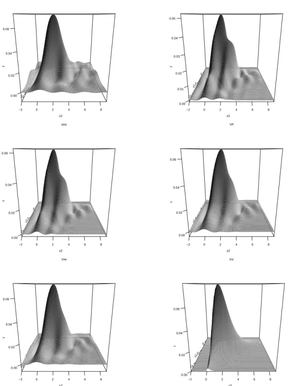
To illustrate, Figure 2.7 presents the deconvolution density estimates based on different kernel types, produced from a simulated data set of OS noise and OS signal with a noise
to signal ratio of 0.2, two replicates per individual (m = 2) and 150 individuals (n = 150).
From the figure, the sinc kernel yields an estimate with the most pronounced oscillations, leading to a substantial negative part in the density estimate unlike the other kernel approaches shown. In contrast, the flat-top kernel provides a density estimate with less wavy and negative artifacts. While less prominent, some negative portions in the density estimate do still appear
with the flat-top kernel in Figure 2.7, but this aspect is difficult to completely remove. For
comparison and perspective, among the kernels in Figure 2.7, only the de la Vall´e-Poussin
kernel (VP) produces a non-negative density estimate. However, from the previous simulations with deconvolution estimators, the VP kernel also induced the worst performances in terms of average ISE, sometimes no better than the contaminated reference estimator that ignored measurment error. In this sense, the flat-top kernel in multivariate deconvolution estimation may lead to comparable performances in terms of ISE compared to the sinc kernel (being the best among all the kernel functions considered here), but with more attractive properties in the shape and appearance of its density estimator.
2.5 Conclusions and promising research avenues
We examined the performance of several different methods for deconvolution density esti-mation with bivariate panel data (repeated measurements for individual subject to distortion by measurement error). While deconvolution estimation has received much attention for uni-variate data, there has been less consideration for multiuni-variate data and, in particular, for panel data structures which arise in scientific studies. For such data, we examined the im-pact of several choices available to the practitioner when implementing a density estimator for the underlying signal variable of interest. These include the type of kernel, the approach for processing replicate measurements in order to estimate error distributions, and the type of estimator of the error characteristic function. One general observation is that the performance of deconvolution density estimators could be improved by using kernel density estimators (and their characteristic functions) formed from error terms rather than the empirical characteristic
x1 5 10 15 x2 −2 0 2 4 6 8 z 0.00 0.02 0.04 0.06 sinc x1 5 10 15 x2 −2 0 2 4 6 8 z 0.00 0.01 0.02 0.03 0.04 0.05 VP x1 5 10 15 x2 −2 0 2 4 6 8 z 0.00 0.02 0.04 0.06 triw x1 5 10 15 x2 −2 0 2 4 6 8 z 0.00 0.02 0.04 0.06 tric x1 5 10 15 x2 −2 0 2 4 6 8 z 0.00 0.02 0.04 0.06 flat x1 5 10 15 x2 −2 0 2 4 6 8 f 0.00 0.02 0.04 0.06 True density
Figure 2.7 Perspective plots of the true density and kernel deconvolution density estimates
based on a sample size of n = 150 varying the kernel function. The sinc kernel
functions from errors; yet the latter is most commonly proposed in the literature. However, among possibilities considered, we found that the most important and substantial feature im-pacting bivariate kernel deconvolution is type of the kernel function. Traditionally, the sinc kernel has been popular for univariate deconvolution, because its Fourier transform is very simple and exhibits good properties in terms of integrated squared error; we show that those features continue to be important for bivariate panel data. However, we also found that flat-top kernels result in similar performance to the sinc kernel in terms of estimation error, while pro-ducing bivariate density estimates with more attractive geometries and fewer wavy artifacts. We have also described numerical integration recipes based on FFTs in order to quickly and practically implement deconvolution estimators in the multivariate data setting; R software and illustrations of implementation are available in a Github repository in Basulto-Elias (2016b).
Open research issues remain mostly associated with the development of theory for multi-variate deconvolution estimation with panel data. Two specific open problems are determining rates of convergence of the kernel density estimators and defining optimal bandwidth choices. A related and important issue for investigation concerns data-driven approaches for selecting bandwidths that are suitable for panel data in the multivariate case.
CHAPTER 3. “FOURIERIN”: AN R PACKAGE TO COMPUTE FOURIER INTEGRALS
A paper to be submitted to The R Journal
Guillermo Basulto-Elias, Alicia L. Carriquiry, Kris De Brabanter and Daniel J. Nordman
Abstract
We present our Rpackage “fourierin” (cf. (Basulto-Elias et al., 2016)) intended to
numer-ically compute Fourier-type integrals of functions of one or two variables and finite support in several points. If the points belong to a regular grid, the algorithm described in Inverarity (2002a) is implemented making significant improvements in the speed.
3.1 Introduction
Continuous Fourier transforms commonly appear in several areas, such as physics and statistics. In probability theory, for example, continuous Fourier transforms are related to the characteristic function of a distribution.
The definition of a continuous Fourier transform may change from one context to another. It is desirable then to have a function that easily adapts to every definition of continuous Fourier transform as well as its inverse.
Fourier integrals cannot always be solved in elementary terms and the oscillating nature of the makes typical numerical integration recipes to fail. Bailey and Swarztrauber (1994) presents an algorithm that expresses the mid-point integration rule in terms of the discrete Fourier transform, which allows the use of the Fast Fourier transform. Inverarity (2002a) extended such characterization to the multivariate case.