The Impact of Financial Sector Liberalization on Financial
Development and Economic Growth: Evidence from Kenya
Wanyama Silvester Mackton1 Josephat Cheboi Yegon2* and Josphat Kipkorir Kemboi3 1. School of Business and Economics, Mount Kenya University, P.O. Box
2. Entrepreneurship & Human Resource Department Eldoret Polytechnic, P.O Box 2662-30100 Eldoret 3. Department of Economics, Moi University, P.O Box 3900-30100 Eldoret
*Email of the corresponding author: cheboijos@yahoo.com
Abstract
We examine the impact of financial sector liberalization on the finance – growth nexus in Kenya by comparing a list of selected indicators of financial development using data covering pre - reform and post - reform periods. The hypothesis on the existence of a cointergrated relationship between financial sector liberalization on financial development and economic growth was tested using Engle and Granger (1987) two-step procedure.The study employed a time series analysis to evaluate the impact of financial liberalization in the finance – growth nexus. An Interactive econometric analysis on the data collected was done using Microfit 4.0. The results showed that there is a significant relationship between the size of financial services sector and economic growth. This implies that the comprehensive measure of the size of the financial sector exerts a positive and statistically significant effect on economic growth. However, financial liberalization has been found to have insignificant impact on financial development.
Keywords: Financial sector, financial sector development, economic growth, Kenya 1.0 Introduction
Financial liberalization is one of the key pillars of Structural Adjustment Programmes (SAP) implemented by most African countries. A lot of work has been done on the relationship between financial deepening and economic performance. Many studies find a close link between financial deepening, productivity and economic growth and conclude that policies affecting the financial sector have substantial effects on the space and pattern of economic development (Goldsmith 1969; King and Levine 1993). It is for example estimated that policies that would raise the M21/GDP ratio by 10% would increase the long-term per capita growth rate by 0.2–0.4% points (World Bank 1994).
The financial sector facilitates savings and investment. In the process, it plays an important role in reducing risks and in the transformation of maturities in the saving-investment nexus (Nissanke et al. 1995). Financial institutions lower the cost of investment by promoting productivity and growth through improved efficiency of intermediation leading to a rise in the marginal product of capital (Montiel 1994).
According to Callier (1991), the performance of the financial sector in Sub-Saharan Africa has an important bearing on the overall economic performance because: (i) the region continues to be in economic crisis and the financial system is relatively underdeveloped compared to any other developing region; (ii) structural adjustment programs require more reliance on the private sector and hence its financing; (iii) the debt crisis and reduction in external savings translates to the need to increase the mobilization of domestic savings for investment; (iv) reform is needed if the financial system is to overcome and avoid the problems of financial distress and restore confidence; and (v) the need for international competitiveness requires that the financial system be as adaptable and flexible as possible.
Financial sector reforms in the region and elsewhere have mainly been triggered by SAPs motivated by the financial repression paradigm promulgated by McKinnon (1973) and Shaw (1973) who emphasized the role of government failures in the sector. Accordingly, the objective of financial reforms is to reduce or reverse this ‘repression’. According to the McKinnon-Shaw hypothesis, financial repression arises mainly when a country imposes ceilings on nominal deposit and lending interest rates at a low level relative to inflation. The resulting low or negative real interest rates discourage savings mobilization and the channeling of the mobilized savings through the financial system. While the low and negative interest rates facilitates government borrowing, they discourage saving and financial intermediation, leading to credit rationing by the banking system with negative impacts on the quantity and quality of investment and hence on economic growth (Mwega et al 1990).
Advocates of this hypothesis postulate that many financial systems in Africa have been subjected to financial repression characterized by low or negative real interest rates, high reserve requirements (sometimes of 20%- 25% compared to 5%-6% in developed countries) which lead to high spreads thereby imposing an implicit tax on financial intermediation; mandatory credit ceilings; directed credit allocation to priority sectors which undermine
1 M2 is the broad measure of money stock defined to include currency in circulation, demand deposits, savings deposits and
allocative efficiency; and heavy government ownership and management of financial institutions. The latter suggests that much credit is given on political rather than commercial considerations, giving rise to a huge pile of non-performing loans in the banks’ portfolios. There is also limited competition, with government and parastatals being major borrowers due to the large deficits that they experience. According to Camen et al. (1996), financial repression in Africa has hindered the development of the capacity of financial institutions in carrying out their informational and resource mobilization role.
Financial sector reforms have also included; reforms in interest rates liberalization which was expected to discourage capital flight and help to stabilize the economy, reducing direct and indirect taxation of financial institutions through reserve requirements, mandatory credit ceilings and credit allocation guidelines, reducing barriers to competition in the financial sector by scaling down government ownership through privatization and facilitating entry into the sector by domestic and foreign firms and restructuring and liquidation of solvent banks (Inanga 1995).
By and large, economic growth cannot be possible without the combined role of investment, labour and financial intermediation. As Jao (1976) puts it, the role of money and finance in economic development has been examined by economists from different angles and with various degrees of emphasis. In particular, the writings of Gurley and Shaw (1955,1956,1967) and Goldsmith (1958,1969) stress the role of financial intermediation by both banks and non-bank financial institutions in the saving-investment process, where money, whether defined narrowly or broadly, forms part of a wide spectrum of financial assets in the portfolio of wealth-holders. Indeed, the economic growth and development of a country depends greatly on this role, the role of financial development.
Although there has been considerable attention on the relationship between Structural Adjustment Programmes (SAP) and economic growth, there is little empirical work on the level of financial development propelled by the financial liberalization and the resulting impact on economic growth. This is curious considering the fact that financial liberalization is one of the subsets of SAPs. Seemingly, there has not been sufficient investigation about the impact of financial liberalization on financial development and economic growth. Since liberalization has been implemented as a deliberate strategy to accelerate the pace of economic growth as presented in SAPs, it is pertinent to have a clear understanding of how financial liberalization affects the link between financial development and economic growth in Kenya.
2.0 The Financial System and Financial Development Process in Kenya
The Kenyan economy depends greatly on agriculture. Kenya is dependent on three major sources of energy – wood fuel accounts for 74 per cent of energy consumed in Kenya, petroleum for 23 per cent and electricity for 2 per cent. Much attention is being given to production of both geothermal energy and hydro-electricity as well as to oil exploration. In Kenya, a population census is conducted every ten years. The first census was conducted in 1948 and the latest in 2009, when there were 40 million Kenyans with an average population density of 49 people per km2. Approximately 70 per cent of Kenya’s population lives in the rural areas but there is an increasing tendency of rural-urban migration in search of gainful employment.
Although the need to liberalize the Kenyan economy was realized in early 1970s following external shocks that resulted into macroeconomic instability, a comprehensive reform program was only implemented in 1990s following the conditional grants by World Bank pegged on implementation of SAPs. To facilitate the liberalization process, Kenya received structural adjustment lending from the World Bank and also Enhanced Structural Adjustment Facility (ESAF) loan from the IMF (O’Brien and Ryan, 1999). It was expected that the reforms would restore macroeconomic stability with greater reliance on market forces and enhanced private sector participation in the development process.
2.1 The Pre Reform Period (1963 - 1989)
At independence, Kenya inherited a financial system composed of the currency Board of East Africa (EACB), that operated in Tanzania, Uganda and Kenya; commercial banks, that were mainly foreign; and a small number of specialized financial institutions. Kenya has a long history of commercial banking, with the predecessors of the three major commercial banks set up before the 1920s. By independence in 1963, Kenya had 10 commercial banks with the “big three” — National and Grindlays Bank, Barc1ays Bank, and Standard Bank — holding about 80 per cent of the total commercial bank deposits. All these banks (except one) were branches of foreign banks, and mainly financed foreign trade.These financial institutionswere suspected for colluding to determine the structure of interest rate. By 1969, the number of these Non Bank Financial Institutions (NBFIs) had risen to 10 and by the end of 1979 to 19. By mid-1980s, the number of these NBFIs had risen to 53, with a total of 100 branches mainly located in urban areas.
Favourable policy enabled NBFIs to offer higher rates of interest making them more competitive than commercial banks while they were not subject to credit ceilings. Hence, NBFIs operated in a more liberal legislative framework than commercial banks. However, in the 1985 amendments to the Banking Act, further consolidated in 1989, controls on NBFIs were tightened. They were barred for example from acquiring or
holding share capital or to have direct interest in commercial, industrial or other undertakings where their financial contribution would exceed 25 percent of their paid capital or unimpaired reserves as well as holding for commercial purposes immovable properties such as land and owning equity in commercial banks.
Table 1 shows some indicators of financial repression during the pre reforms period in Kenya. Kenya experienced low or negative real interest rates, low M2/GDP ratio and high fiscal deficits/GDP ratio compared to the more advanced countries. The degree of financial deepening for example compares very unfavourably with the M2/GDP ratio for the USA (67.0%), Japan (183.1 %), Singapore (126.1 %), Portugal (74.1 %); Greece (79.3%) and Spain (68.8%) (ADB 1994).
Table 1:Some Indicators of Financial Repression In Kenya
Country Year M2/GDP Ratio Rate (%) Real Deposit Rate (%) Real lending GDP Fiscal Deficit Ratio (%) Kenya 1985 28.2 0.3 3.3 -3.8
Source: Seck and El Nil (1993) and author’s calculations. Note: Figures apply to the year 1985.
The 1974-1985 period was dominated by low nominal lending rates, which, because of high inflation rates, were negative in real terms (Table 2.1). In theory, high inflation rates motivate the public to shift from holding monetary assets to physical ones, which act as inflationary hedges.
In addition to fixing interests, during the period 1974-1985 the government directed banks to open branches in its preferred areas and to grant credit to specific sectors, irrespective of commercial considerations of risk and returns. For example, banks’ credit was directed to parastatals and cooperatives, irrespective of their credit worthiness since the main criterion for provision of credit was politically motivated. Thus, financial institutions lost their ability to screen borrowers and to assess risk against reward. Moreover, the option of cutting off credit and collecting debts was invoked. Consequently, economic growth declined drastically from 5.2 percent in 1973 to 1.3 in 1984
2.2 The Path to the Reform Process
Like in some other countries, the thirst for liberalization policy in Kenya was preceded by economic crises. However, the government showed some reluctance in implementing the reform even where the need for it was very obvious, while at the same time it took measures that did not necessarily remedy the situation. For example, after a remarkable economic performance witnessed in late 1960s, in 1971, the government witnessed a balance of payment deficit problem following an expansionary fiscal budget in 1970 and 1971. Instead of liberalizing the economy, policymakers imposed policy controls that were characterized by controls on domestic prices, foreign exchange transactions, interest rates and importation licensing. There was also mounting pressure from the urban elite group who were thought to be a political threat; this group consisted of urban salary and wage earners mainly employed by the government parastatals (Nelson, 1984). Further, the bank ceilings made it impossible for the government to draw the funds to implement proposed changes, while the government was put under pressure with conditionality in receiving the financial support.
Following the oil crises in 1979, it was time again for the government to come up with further policy measures to deal with the escalating economic crises. The government presented a structural adjustment programme in Sessional paper No. 4 1980 on Economic prospects and policies similar to the 1975 Sessional paper No. 4. Emphasis was made on fiscal stabilization and balance of payments problem. And in the 1980/81 budget, import controls were liberalized and interest rates increased. A new credit was negotiated with IMF in October 1980 with less stringent policy conditions except that import policy was to change from quantitative to tariffs. However, there seemed to be no full commitment on the government on the need to use the resources to achieve long-term adjustment. And the agreement fell part as the government expenditures increased more rapidly than budgeted. By the second half of 1981, the government conceded a measure of liberalization under pressure from IMF and World Bank and this saw devaluation of the shilling in 1982. In January 1982 a third standby agreement was reached with IMF but with tough conditions but again the agreement was suspended as by middle of 1982 when bank credit to the government had broken the agreed ceiling. The government showed commitment to the reform process in Sessional Paper No.1 of 1986 on Economic Management for Renewed Growth, in which it adopted an outward-looking development strategy and proposed the liberalization strategies. However, it was not until the 1990s that a greater degree of liberalization was witnessed, both in the financial and goods markets.
2.3 The Reform Period (1989 Onwards)
The country formally adopted financial sector reforms in 1989, supported by a $170 million World Bank adjustment credit. Financial reform proposals were first incorporated in the 1986–90 structural adjustment program. The main feature of the program was full interest rate liberalization which was achieved in July 1991 after a gradual increase in nominal rates in the 1980s. In the first half of the 1980s for example, nominal deposit rates were increased by about 100 percent and lending rates by about 50 percent, from relatively low levels. Before this period, the government followed a low-interest-rate policy whose main objective was to promote investment. From the time the Central Bank was established in 1966 until 1980 interest rates were only adjusted
upwards once in 1974 by 1 to 2 percentage points.
Other reforms included (i) liberalization of the treasury bills market in November 1990; (ii) setting up a Capital Markets Authority in 1989 to oversee the development of the equities market with a view to enhancing availability of long-term resources for investment; (iii) abolition of credit guidelines in December 1993 (which were in existence since 1975 in favor of agriculture); and (iv) improving and rationalizing the operations and finances of the DFIs, though against the wishes of some donors who urged for their dissolution or privatization. In 1988 and 1994, the two parastatal banks were partially privatized, selling 30% of their shares to the public. A component of reforms has been the restructuring of financial institutions. The country experienced a bank crisis in 1986 when a number of ‘specified’ NBFIs and a small commercial bank collapsed. To avoid a repeat, eight financial institutions were taken over and merged into a state bank in 1989 — Consolidated Bank of Kenya Ltd. The central bank has also strengthened the supervision and the inspection of financial institutions and introduced a Deposit Protection Fund which guarantees deposits up to Ksh 100,000. The initial capital for setting up financial institutions has been increased both for commercial banks and “specified” NBFIs.
2.4 Outcome of Reforms
According to the World Bank (1994) Report, structural adjustment programs have been more successful in achieving macroeconomic stabilization and trade and agricultural reforms than with privatization of public enterprises and financial sector reforms. The actual experience of most African countries with financial reforms has been that of limited success, mainly as a result of failure of real deposit rates to remain consistently positive. This is because of the relatively high fiscal deficits which have characterized these countries. Interest rate liberalization and a decline in inflation have however helped eliminate extremely negative interest rates.
The World Bank (1994) assessment of financial reforms in Africa was conducted to a large extent within the McKinnon-Shaw framework, with the overall approach to financial development — removing financial repression, dismantling directed credit programs, introducing better accounting, legal, and supervisory frameworks, continuing with institution building, deepening and developing capital and money markets — is postulated to be on target and in the right direction. As shown in Section II, the reforms carried out by the four countries under study have varied, but all have entailed interest rate liberalization as well as bank restructuring and liquidation. The Report does not address itself adequately to the basic tenets of this paradigm, with the presumption that if the problems described above were resolved, then reforms would achieve the objectives postulated by Mckinnon-Shaw.
2.5 Empirical Evidence
Theoretical arguments do not provide precise conclusions on the relationship between financial development and economic growth; even though the majority tends to favour the view that financial development leads to economic growth. Goldsmith (1969), asserts that economic theory and history, both assure that the existence and development of a superstructure of financial instruments and financial institutions is a necessary, though not sufficient condition for economic development. He examined data from 35 countries between 1860 and 1963. His findings support the supply-leading relationship between financial and economic development for developing countries and a reverse causal direction for developed countries. He also found out that the pace of financial development proxied by the value of intermediary assets as a proportion of GDP was correlated with economic growth. Thus, countries with highly developed financial superstructure have high economic growth. Goldsmith (1969) maintains that the direction of causation is from economic to financial development.
Jung (1986) provides an empirical verification of Patrick’s (1969) theory. He explores the issue by testing the Granger causality framework with data from 19 developed and 37 developing countries. Jung (1986), studies both characterization of causality and temporal behaviour between financial development and economic growth. He found out that, the relationship between financial development and economic growth was supply- leading irrespective of the stage of development. Thus, he argued that the expansion of the financial system promotes the demand for its services. Therefore, scarce resources from small savers are hence channeled to large investors in line with rates of return and, in the process: the financial sector proceeds and induces growth.
Demetriades and Hussein (1996), in their study of 16 developing countries, found out that, the causality between financial development and growth is mostly bi-directional. However, there are important cases in which the relationship runs from economic growth to financial development. They suggest that variations in causality reflect country specific factors such as the quality of non-financial institutions including the degree of sound governance, the type of financial policies followed and the effectiveness of the government institutions, design and policies implemented.
Most of the remaining empirical studies do not get involved in the controversy of supply-leading versus demand-following relationships. Instead, they are based on assumed supply-leading relationship. The studies proceed directly to evaluate the impact of financial development on economic growth.
De Gregorio and Guidotti (1995), included 100 countries in their study during 1871 to 1994 period. They concluded that financial development leads to an improved growth performance. In addition, the correlations between financial development (OECD) countries, depending on the time period studied. They also found a
positive effect of financial development on long-run growth of real per capita income. The findings are particularly strong in middle and low-income countries, but weak in high –income countries where financial development is taking place outside the banking system.
Levine (1997) examines the finance-growth link. He uses cross- section analysis to examine the link beyond the relationship between finance and growth by running 12 regression equations. His results suggest a positive first-order relationship between financial development and economic growth. Levine argues that the development of financial markets and institutions is critical and inextricable part of economic growth and the level of financial development is a good predictor of future rates of economic growth, capital accumulation and technological change.
Montiel (2000) argues that theory and evidence suggest that financial development can contribute to economic growth. He argues that most of the sub-Saharan African countries are at an early stage of development, where commercial banks continue to dominate the formal system. Montiel examines the potential role of financial liberalization in reactivation of economic growth through financial development in sub-Saharan Africa. He observes that in most Sub-Saharan Africa countries’ financial liberalization has not appeared to be very successful. Montiel suggests that, in the long run further liberalization is likely to be desirable.
3.0 Methods 3.1 Sources of data
We utilized secondary data collected mainly from various issues of the Central Bank of Kenya, Statistical Bulletin, Economic Surveys, Statistical Abstracts and International Financial Statistical Year Book (2007) published by International Monetary Fund (IMF), the internet and supplemented by data from different publications. These data sets covered the period 1977- 2007.
3.2 Data analysis
This study applies Engle-Granger two-step procedure of Johansen procedure. Engle and Granger (1987) have produced the cointegration technique that incorporates both short run dynamics emanating from first order differences and common long run trend movements among variables. In this study the Engle- Granger two-step procedure is used to test for cointegration.
3.3 Model Specification
In examining the effects of financial development on economic growth in Kenya’s pre-and post-liberalization eras, it was hypothesized that financial development enhances economic growth in the liberalized period in Kenya.
The Model specification follows Odedokun (1991),who proposes the use of the Conventional neoclassical one sector aggregate production function in which financial development enter as an input ,That is,
Yt = f (Lt , Kt , Ft , Zt) ………..(3.1)
Where Y= aggregate output or real GDP; L=labour force; K=capital stock; F=measure of the level of financial development; and Z =vector of other factors that can be regarded as inputs in the aggregate production process. The subscript t denotes the time period. By differentiating equation (3.1) and appropriately manipulating the resulting expression, Odedokun (1991) arrives at the growth equation below.
y = aIt + b(I/Y)t + cft +dzt ...(3.2)
Where the lower case letter of a variable signifies that the variable is now in growth rate form, such that y,If and z are growth rates of real GDP, labour force, financial intermediation and vector of other inputs, respectively. The expression (1/Y) is the share of real gross investment (1) in real GDP (Y) whiles a, b and c are constant parameters (d is a vector of parameters).
By adopting endogenous growth models in Odedokun’s specification which relax the assumption of diminishing returns to capital, the basic equation to be used in this study, also to be used for testing the main hypothesis in most cross-Country studies, has been of the form presented by Levine(1997)as follows:
Yt = βo + β1FDt +β2Xt + εt. ……… (3.3)
Where, Yt is the rate of growth of real per capita GDP 0f the country at time t, FDt is an indicator for financial development, Xt is a set of control variables and εt is the error term. However, we abstract from the model adopted by Levine (1997), that relates the growth rate of GDP to investment (as ratio of GDP), and the growth rate of per capita capital stock.
We followed Amusa (2000), and augment Levine’s equation to include a set of proxies for financial development and dummy variables to capture the effect of economic and financial reforms in Kenya. The study also included openness and Government consumption in Kenya as control variables. The equation for estimation is specified as follows:
Yt = β0 +β1PTC +β2PGDP +β3MGDP + β4IGDP + β5OP + β6GVC + β7DU + εt……. (3.4)
Where Yt is the rate of growth of real per capita GDP, Ratio of Private Credit to Total Domestic credit (PTC), Ratio of Private Credit to GDP (PGDP) and Ratio of Liquid Liabilities to GDP (MGDP) are the indicators for financial development. OP is the openness, IGDP measure the ratio of investment to GDP, GVC is the
government consumption, DU is a dummy variable for financial liberalization (the pre- reform period takes the value zero and the post -reform period takes the value one), εt is the error term.
3.4 Engle- Granger Cointegration Test
Engle and Granger (1987) advocate Augmented Dickey Fuller (ADF) tests of the following kind: ∆ εt = µεt-1+ Σµi∆εt-1+ µ+ δt+ st ……….. (3.5)
Where st~ NID (0, σ2)
The residual based on ADF test for cointegration assumes that all the variables in the Ordinary Least Square (OLS) equation are all integrated of order one (1) such that the cointegration test gears to establish whether the error term is integrated of order one εt~ 1(1) against the alternative that is integrated of order zero εt~ 1(0). If some of the variables are in fact integrated of order two 1(2) then cointegration is still possible if the 1(2) series cointegrates down to 1(1) variable in order to cointegrate potentially with other 1(1) variables.
3.5 Error Correction Model (ECM)
If the variables are cointergrated, estimating the equation in first difference results in the loss of valuable information on the long run relationship between the levels of the variables. For example if;
Yt = β0 +β1X1t +β2X2t + εt……….. (3.6) Where εt is the error term, then;
Yt–Yt-1 = β1(X1t – X1t-1) + β2(X2t – X2t-1) + µt……….(3.7)
Thus if equation (3.7) is estimated instead of equation (3.6), according to Engle and Granger (1987), then the information about β0 is lost. Thus equation (3.7) focuses purely on the short run relationship between Y and X, hence it is likely to provide a poor forecast for even a few periods ahead if a long run relationship exists but is ignored. Furthermore, the first differenced equation (3.7), will result into auto correlated error term if the relationship in equation (3.6) really exist; and, if disturbance term εt is non auto correlated then the disturbance term µt in equation (3.11) is of simple moving average form such that it is auto correlated. Therefore, first differencing is an unsatisfactory method of dealing with spurious problem. The appropriate method is to use Error Correction Model (ECM) that results in equations with first differenced and hence stationary dependent variables but avoid the problem of failing to make use of any long run information in the data. The result of cointegration test enables us to formulate an ECM.
ECM relates short run changes in the dependent variable Yt to short run changes in the explanatory variables (the impact effect), and also the long run effect through a feedback mechanism.
3.6 Estimation Technique
In line with the econometric techniques, the existence of unit root(s) in each variable was tested by using, the Augmented Dickey Fuller (ADF) and Phillip Perron (PP) tests. Based on the unit root results we shall examine the evidence for cointegration among the variables using the Augmented Dickey Fuller (ADF) test as advocated by Engle and Granger (1987). If the variables are cointegrated then, we have the long run information with respect to financial development in long run. Therefore, an Error Correction Model (ECM) will be estimated. This model is expected to provide useful estimates of short run dynamics and long run relationships in the economic growth equation.
3.7 Measurement of Variables
Economic Growth: Consistent with other studies, Levin (1997), economic growth is measured using per capita growth in real GDP. It is also the ideal choice for a study on a country like Kenya because of data availability. In testing the proposed hypothesis, the analysis will be restricted to testing for the impact of financial development on per capita real GDP(Y).
Financial Development : There are three measures of financial development namely, the ratio of liquid liabilities to GDP, ratio of private credit to GDP and the ratio of private credit to total domestic credit have been proposed (Levine,1997). These measures reflect the size of the financial system and the distribution of credit flows. The size of financial sector may be measured, as in King and Levine (1993b), as the ratio of liquid liabilities (currency plus demand and interest-bearing liabilities of banks and nonbank financial intermediaries) divided by GDP (MGDP). Based on the assumption that there is a positive correlation between the size of financial sector and provision of financial services, therefore, the existence of the formal financial sector in Kenya suggest that the use of the ratio of liquid liabilities to GDP as a proxy for financial sector development is appropriate. We adopt Levine (1997) view and focus on the volume of credit granted by the financial sector to the private sector. Availability of data in the range of study enables us to choose these variables as appropriate measurers for financial development.
Control Variables: In addition to financial sector lending being an essential force behind the growth process, this study attempted to isolate the effect of some conventional factors, namely, openness and government consumption. Openness (OP): This is the sum of imports and exports as percentage of GDP.
Government Consumption (GVC): This was defined as general government consumption as a percent of GDP.
4.0 Empirical Results
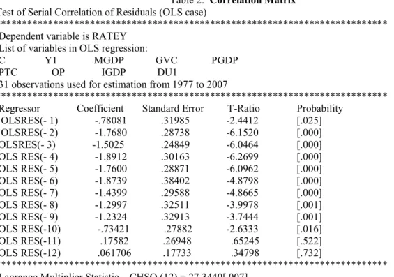
This study adopted a more incisive quantitative analysis such as correlation coefficient matrix1, unit root tests and cointegration tests. The correlation matrix, in this case, presents the relationship between economic growth and other variables used in the analysis. The computed coefficients and the expected signs are presented in Table 2.
Table 2: Correlation Matrix
Test of Serial Correlation of Residuals (OLS case)
*************************************************************************** Dependent variable is RATEY
List of variables in OLS regression:
C Y1 MGDP GVC PGDP PTC OP IGDP DU1
31 observations used for estimation from 1977 to 2007
*************************************************************************** Regressor Coefficient Standard Error T-Ratio Probability
OLSRES(- 1) -.78081 .31985 -2.4412 [.025] OLSRES(- 2) -1.7680 .28738 -6.1520 [.000] OLSRES(- 3) -1.5025 .24849 -6.0464 [.000] OLS RES(- 4) -1.8912 .30163 -6.2699 [.000] OLS RES(- 5) -1.7600 .28871 -6.0962 [.000] OLS RES(- 6) -1.8739 .38402 -4.8798 [.000] OLS RES(- 7) -1.4399 .29588 -4.8665 [.000] OLS RES(- 8) -1.2997 .32511 -3.9978 [.001] OLS RES(- 9) -1.2324 .32913 -3.7444 [.001] OLS RES(-10) -.73421 .27882 -2.6333 [.016] OLS RES(-11) .17582 .26948 .65245 [.522] OLS RES(-12) .061706 .17733 .34798 [.732] *************************************************************************** Lagrange Multiplier Statistic CHSQ (12) = 27.3440[.007]
F Statistic F (12, 10) = 6.2326[.003]
*************************************************************************** Source: Generated by Microfit 4.0
The Lagrange Multiplier Statistic and the F-statistic are both significant. This then means that the data used is statistically reliable. It shows that most of the variables satisfy the normality test.
4.1 Unit Root Test
This study tested for the presence of unit root in the variables using the Augmented Dickey Fuller (ADF) and Phillip Perron tests. Assuming the series contain a trend (deterministic or stochastic) the study included both a constant and a trend in the test regression. ADF test tends to be more popular due to its simplicity and general applicability, while the PP test is the non – parametric test based on Phillips (1987) Z-test, which involves transforming the test statistic to eliminate any autocorrelation in the model. It was very necessary to conduct a formal test to confirm the time series properties of the variables although this is not meant for any adjustment since the study has adopted the ECM for the analysis. The study adopted the Augmented Dickey-Fuller (ADF) unit root procedure to test the level of integration for the variables involved in the study (see table 4-2). The null hypothesis of the series being non-stationary is accepted in levels indicating that the variables are non stationary, integrated of order one. Having determined the order of integration of the series, the multivariate cointegration test was conducted by applying the Johansen and Juselius (1990) maximum likelihood estimation procedure. As the selection of the correct order of ARDL is important in this type of examination, and given the medium size of the study samples, lag order selection by either the Akaike information criteria (AIC), or by the Schwartz Bayesian criteria (SC) is recommended (Noer Azam Achsani, 2010), the study adopted the Akaike information criteria(see table 4-1).
The ADF test was, therefore, used to establish the order of integration of the variables and the degree of differencing required in order to induce stationarity. Non-stationary variables2 have a non-constant mean and
variance. The unit root tests are presented in Table 3.
1 The correlation coefficient matrix is a vital indicator for testing the linear relationship among the variables as well as the
strength of the variables in order to detect the presence of multicolliniarity.
2 Working with such variables in their levels yields a high likelihood or erroneously indicate, through misleading values of R2,
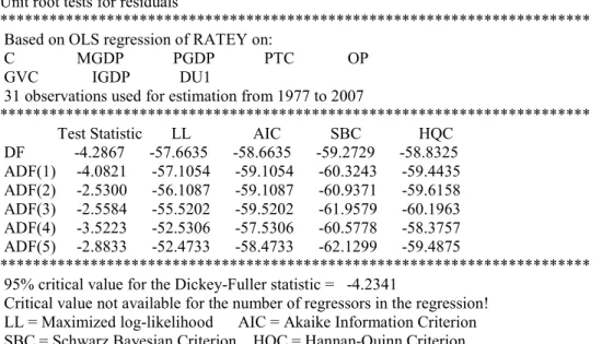
Table 3: Unit Root Tests for Variables.
Unit root tests for residuals
************************************************************************ Based on OLS regression of RATEY on:
C MGDP PGDP PTC OP GVC IGDP DU1
31 observations used for estimation from 1977 to 2007
************************************************************************ Test Statistic LL AIC SBC HQC
DF -4.2867 -57.6635 -58.6635 -59.2729 -58.8325 ADF(1) -4.0821 -57.1054 -59.1054 -60.3243 -59.4435 ADF(2) -2.5300 -56.1087 -59.1087 -60.9371 -59.6158 ADF(3) -2.5584 -55.5202 -59.5202 -61.9579 -60.1963 ADF(4) -3.5223 -52.5306 -57.5306 -60.5778 -58.3757 ADF(5) -2.8833 -52.4733 -58.4733 -62.1299 -59.4875 ************************************************************************ 95% critical value for the Dickey-Fuller statistic = -4.2341
Critical value not available for the number of regressors in the regression! LL = Maximized log-likelihood AIC = Akaike Information Criterion SBC = Schwarz Bayesian Criterion HQC = Hannan-Quinn Criterion
Source: Generated by Microfit 4.0
From the nature of series and results in Table 4.2, it is clear that any dynamic specification of the model in levels will be inappropriate and may lead to the problem of spurious regression, given that indeed some variables are non-stationary. When the test statistic absolute values are less than the critical absolute values, then the variable is non-stationary. Cointegration analysis was hence done to ascertain the appropriateness of the Error Correction Model (ECM). ECM is possible if and only if series are cointegrated.
4.2 Cointegration Tests
The study employed the concept of cointegration. The study adopted the Johansen Juselius (JJ) multivariate cointegration technique to test for cointegration. To establish whether there is long-run equilibrium relationship among the variables in
Yt = β0 +β1PTC +β2PGDP +β3MGDP + β4IGDP + β5OP + β6GVC + β7DU + εt …..(4.1)
The Johansen method suggested two statistics to determine the number of cointegrating vectors: the trace statistics and maximum eigen values. The appropriate critical values for the tests are provided in Osterwald Lenmum (1992).
The essence of employing cointegration tests lies in analyzing the presence of long-run relationship between the variables. This study extended the empirical work on finance-growth nexus by applying cointegration analysis, which considers non-stationary and common long-run trends. In testing for cointegration, the Engle and Granger (1987) two-step procedure is applied.
Thus, after establishing the order of integration, the next step is to establish whether the non-stationary variables are cointegrated. According to Engle and Granger (1987), individual time series could be non-stationary, but their linear combinations can turn out to be stationary if the variables are integrated of the same order. This is because equilibrium forces tend to keep such series together in the long run. As such, the variables are said to be cointegrated and error-correction terms exist to account for short-term deviations from the long-run equilibrium relationship implied by the cointegration. Furthermore, the differencing of the non-stationary variables to achieve stationarity leads to loss of some long-run properties.
Equation (3.4), where per capita GDP growth (Y) is a dependant variable was regressed on explanatory variables and its error term was tested for stationarity based on the unit root test explained above (ADF and PP). The results are presented in Table 4.
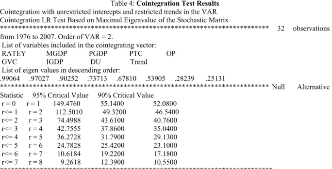
Table 4: Cointegration Test Results
Cointegration with unrestricted intercepts and restricted trends in the VAR Cointegration LR Test Based on Maximal Eigenvalue of the Stochastic Matrix
************************************************************************** 32 observations from 1976 to 2007. Order of VAR = 2.
List of variables included in the cointegrating vector: RATEY MGDP PGDP PTC OP GVC IGDP DU Trend
List of eigen values in descending order:
.99064 .97027 .90252 .73713 .67810 .53905 .28239 .25131
************************************************************************** Null Alternative Statistic 95% Critical Value 90% Critical Value
r = 0 r = 1 149.4760 55.1400 52.0800 r<= 1 r = 2 112.5010 49.3200 46.5400 r<= 2 r = 3 74.4988 43.6100 40.7600 r<= 3 r = 4 42.7555 37.8600 35.0400 r<= 4 r = 5 36.2728 31.7900 29.1300 r<= 5 r = 6 24.7828 25.4200 23.1000 r<= 6 r = 7 10.6184 19.2200 17.1800 r<= 7 r = 8 9.2618 12.3900 10.5500 ***************************************************************************
Use the above table to determine r (the number of cointegrating vectors) Source: Generated by Microfit 4.0 The results from the cointegration analysis (Table 4-3) shows that when two to six lags are used, the null hypothesis of no cointegration (r = 0) between variables (y-MGDP), (y-PGDP), (y-PTC), (y-IGDP), (y-GVC), and (y-OP) rejected at 10 per cent using either the trace test or maximum Eigen value test. The Cointegration LR (likelihood ratio) Test Based on Maximal Eigen value of Stochastic Matrix rejects Ho that r<=5 and accepts H1 that r=6 (at 10% level of significance where the Statistic > critical value i.e. 24.7828> 23.1)
The Cointegration LR (likelihood ratio) Test Based on Trace of Stochastic Matrix rejects Ho that r <= 2 and accepts H1 that r>=3 (at 5% and 10% level of confidence the Statistics > critical value i.e. 74.4988 > 43.61 and 74.4988 > 40.76 respectively).
This provides evidence on the existence of at least one cointegrating vector in the model and therefore the study concluded that the variables exhibit a long-run association between them. Having established this, the study then estimated an Error-Correction Model based on equation 4-1 to investigate the relationship between the variables The test results reject the null hypothesis of no cointegration among the variables. This implies that the variables are cointegrated. Although they individually exhibit a random walk, there seems to be a stable long-run relationship between them. Thus, they will not wonder away from each other. Hence, the estimation of an Error Correction Model (ECM) can be carried out.
4.4 Error Correction Model (ECM)
Since time series are integrated of order six, then the ordinary regression analysis is inadmissible. The results of the cointegration test enable formulation of an Error Correction Model (ECM)1. The error correction mechanism, first used by Sargan and later popularized by Engle and Granger, corrects for disequilibrium. It is a means of reconciling the short-run behaviour of an economic variable with its long-run behaviour. The underlying principle of error correction mechanism is that there is a long run relationship between variables. It recognizes the fact that in the short run there is disequilibrium and that it will be eliminated with time so much so that total equilibrium will be realized in the long run. The ECM has incorporated an error correction mechanism which is used to eliminate the disequilibrium from time to time, say year to year.
The ECM thus allows for the exploitation of information on the equilibrium relationship between non – stationary series within a stationary and therefore, statistically consistent model. The growth equation (3.4) is then respecified in an ECM as follows:
Yt = βo+β1iΣ∆PTCt-1+β2iΣ∆PGDPt-1+β3iΣ∆MGDPt-1+β4iΣ∆IGDPt-1+ β5iΣ∆GVTt-1 +β6iΣ∆0Pt-1+β7iDU+λ1ECM t-1+εt …….. (4.2)
Where all the variables are as defined in equation (3.4) in the preceding chapter; ECMt-1 is the error correction term lagged one period and its coefficient (λ1) measures the speed of adjustment of the growth rate of per capita GDP to its long-run equilibrium.
4.6 Regression results for Estimated ECM
The Error correction Model (ECM) result of the estimated growth model is presented in Table 5 below
1 The ECM relates short run changes in the dependent variable (Yt) to short run changes in the explanatory variables (the
Table 5 Error Correction Representation for the Selected ARDL Model
ARDL(4) selected based on Akaike Information Criterion
*********************************************************************** Dependent variable is dRATEY
30 observations used for estimation from 1978 to 2007
*********************************************************************** Regressor Coefficient Standard Error T-Ratio[Prob]
dRATEY1 1.7876 .28882 6.1894[.000] dRATEY2 .86268 .14829 5.8175[.000] dRATEY3 .27933 .072640 3.8454[.001] dC -74.1781 20.4053 -3.6352[.002] dY1 .0097067 .0010840 8.9547[.000] dMGDP 4.8414 1.9867 2.4369[.026] dPGDP 3.2572 1.2542 2.5969[.019] dPTC -7.5664 4.9283 -1.5353[.143] dOP -.055691 .10658 -.52253[.608] dGVC -.46203 .19427 -2.3783[.015] dIGDP 1.0726 .35630 3.0105[.008] dDU -2.1104 1.9328 -1.0919[.290] ecm(-1) -.85357 .094133 -9.0677[.000] *********************************************************************** ecm = RATEY + 22.0939*C -.0028911*Y1 + 1.4420*MGDP -.97014*PGDP + 2.25 36*PTC + .016588*OP + .013762*GVC + .31949*IGDP + .62858*DU1
***********************************************************************
R-Squared .87955 R-Bar-Squared .86512
S.E. of Regression 1.6683 F-stat. F (12, 17) 67.8637 [.000]
Mean of Dependent Variable -.033934 S.D. of Dependent Variable 8.9322
Residual Sum of Squares 47.3124 Equation Log-likelihood -49.4018
Akaike Info. Criterion -62.4018 Schwarz Bayesian Criterions -71.5096
DW-statistic 1.3972
Source: Generated by Microfit 4.0.
The coefficient of multiple determination of the model in Table 4.4 shows that the test statistics are satisfactory. The goodness of fit R-Squared1 variable shows that the explanatory variables in the model account for about 87.96 percent of the variations in real per capital GDP growth rate. The F- statistic shows that the model is very powerful, that is the explanatory variables are jointly significant at the 5% level of significance. This justifies that the model is well specified2.The DW [Durbin Watson] statistic is approximately 1.4 and larger than R2, implying that the regression is not spurious. The error correction term is negative as expected and significant. The strong significance reinforces the argument of the model variable being cointegrated. The error correction term lagged one period [i.e. ecm (-1)] shows that 85.357 percent of the disequilibrium error in the previous period (t-1) is compensated for or corrected for in the current period (t).
In the table 4-4 above, all variables except openness and government consumption have each (in absolute terms) an estimated coefficient greater than standard error. Obviously, we prefer to make observations based on coefficients which are large relative to the imprecision in their estimate. Hence, the larger the t-ratio, the more confident we are in making these observations.
The T-Ratio column reports the t-ratios for each coefficient estimate. They are all well beyond our cutoff point of 2.0 (except for openness, government consumption and the dummy for financial liberalization, which we can ignore), so we can have some confidence in making observations based on this table. In the above table the computed Prob (t) for lagged dependent variable is 0.000 indicating that there is 0% chance that the actual value of this variable could be zero. The Prob (t) for liquid liabilities as a ratio of GDP was 0.026 indicating that there are only 26 chances in 1000 that the parameter could be zero. Under such instances we have a lot of confidence in the estimate and we can reject the Ho hypothesis. The Prob (t) for private credit as a ratio of GDP and government consumption was 0.019 and 0.015 respectively thus indicating that there are 19 and 15 chances in 1000 that the actual value of their respective parameters could be zero. We again have a lot of confidence in the
1 R2 measures the percent of the variation of the dependent variable that is explained by the regression equation. R2 thus lies
between zero and one.
2 According to Granger and Neshold – ‘ An R2 > d [DW-statistic] is a good rule of thumb to suspect that the estimated
regression is spurious’. The estimated regression in this study shows a non-spurious regression since; R2 < d [DW- statistic],
estimates and we can reject the Ho hypothesis. The Prob (t) for investment as ratio of GDP was 0.008 indicating that there are only 8 chances in 1000 that the actual value of this variable could be zero. The Prob (t) for private credit as a ratio of total domestic credit and financial liberalization was 0.143 and 0.290 respectively thus indicating that there are 14.3% and 29% chances that the actual value of their respective parameters could be zero. Under such instances we have a reasonably lot of confidence in the estimates and we can reject the Ho. The Prob (t) for openness was 0.608 thus indicating that there is 60.8% probability that the actual value of its respective parameter could be zero. This implies that the term of the regression equation containing the parameter can be eliminated without significantly affecting the accuracy of the regression.
The levels of 1%, 5% and 10% are popular levels of confidence (99%, 95% and 90% confidence interval). The critical value of t-statistics at 5% level of significance is 1.645. The estimated t-statistics for variables MGDP=2.4369> 1.645 and PGDP= 2.5969> 1.645 hence we can be sure that at 5% level of significance that our estimated coefficients of these variables are statistically different from zero. We reject the null hypothesis and conclude that there is a statistically significant relationship between liquid liabilities as a ratio of GDP, private credit as a ratio of GDP and economic growth in Kenya.
The estimated t-statistics for IGDP=3.0105> 1.645 and for GVC= -2.3783 and thus │2.3783│>1.645, hence we can be sure that at 5% level of confidence that our estimated coefficients of these variables are statistically different from zero. We reject the null hypothesis and conclude that there is statistically significant relationship between the ratio of investment to GDP , government consumption and economic growth in Kenya.
The estimated t-stat for variable PTC= -1.5353 thus │1.5353│< 1.645, for variable OP= -0.5225 thus │0.5225│< 1.645 and for the variable DU= -1.0919 thus │1.0919│< 1.645 hence we can be sure that at a 5% level of confidence we cannot reject the null hypothesis that the estimated coefficient is zero. We conclude that there is no statistically significant relationship between the ratio of private credit to total domestic credit, openness of the economy, financial liberalization and economic growth in Kenya.
4.7 Discussion of Findings
Financial Depth: The variable of financial depth in the first difference, i.e. Ratio of Liquid Liabilities to GDP (dMGDP), indicates that it is statistically significant with a positive impact on financial development, which implies that the comprehensive measure of the size of the financial sector exerts a positive and a statistically significant effect on economic growth in Kenya. A 1% increase in MGDP holding other independent variables constant leads to approximately 4.84% increase in financial development in the short-run.
Private Credit and Investment: The Ratio of Private Credit to GDP (dPGDP) and the Ratio of Investment to GDP (dIGDP), all modeled in their first difference, indicate that they too are statistically significant with a positive impact on financial development, as expected. PGDP has been found to have a significant positive effect on financial development in the short-run. A 1% increase in PGDP leads to 3.26% positive change in financial development. The model indicates that a 1% increase in IGDP leads to a 1.07% increase in financial development.
Government Consumption: The results also show that another explanatory factor considered in this study, that is, Government consumption as a ratio of GDP in first difference (dGVC) is statistically significant and has a negative impact on growth. Government consumption in the long-run has the hypothesized negative relationship with financial development. A 1% increase in government consumption reduces economic growth by 0.46% and is very significant with an absolute t-value of 2.38.
Private Credit and Total Domestic Credit: In the growth equation, the Ratio of Private Credit to Total Domestic credit in the first difference (dPTC) has an opposite sign to a priori expectations, although statistically insignificant, contrary to the stated hypothesis; indicate that increasing the level of financial sector lending does not enhance economic growth in Kenya. These findings may be related to the infancy of privatization to the extend that new private firms are still growing, hence unlikely to have efficiently utilized the resources or they are still in an investing phase. A positive impact is likely to show up in later years. In addition, since most new banks are active only in towns, few financial instruments have been developed by the financial institutions and the core indicators do not show fierce competition. Thus majority of potential (private) borrowers do not access the credit facilities.
Error Correction Term: The other variable included in the estimation model is the lagged error correction term; ecm-1 which has the expected sign and is statistically significant. The magnitude of the coefficient of the error correction term lies between zero and one in absolute terms, as expected. This magnitude shows that 85.36 percent of the short-run disequilibrium adjusts to the long-run equilibrium each year, which then indicates that the speed for the real per capita GDP growth rate to converge to the long-run equilibrium point is very high. Financial Liberalization: As for the dummy variable for financial liberalization (DU) in the first difference (dDU), its coefficient, though statistically insignificant has an opposite sign, contrary to the hypothesis. This sign would be as a result of the reform of the financial sector in Kenya being in the infancy stage. In the long-run the expected impact is likely to show up.
5.0 Discussion and Conclusions
The long run model results mostly conform to the stated hypotheses. Factors that significantly and positively influence financial development and, in turn, economic growth includes: Ratio of Liquid Liabilities to GDP (MGDP), Ratio of Private Credit to GDP (PGDP), and Ratio of Investment to GDP (IGDP), Ratio of Private Credit to Total Domestic credit (PTC), openness of the economy (OP) and Government consumption as a ratio to GDP (GVC), influence economic growth negatively. The long-run negative influence of PTC and OP are however insignificant. Therefore the long-run significant determinants of financial development include MGDP, PGDP, IGDP, and GVC. PTC, OP, and Du have been found to have insignificant impact on financial development.
Comparing econometric analysis of various studies can be a problematic exercise due to variations in the qualitative methods of analysis employed. While some studies analyze finance – growth nexus of a single country, others are cross sectional in nature. They also differ in the choice of variables, data and sample period. Differences can also be realized in econometric techniques employed and other differences in measurements are likely to make inter country comparison difficult.
However it is worth to compare our results with other studies done in Kenya and other parts of Africa. As regard the size of the financial sector (financial depth), the study by Amusa (2000) found it to be positive and statistically significant to economic growth in the case of South Africa. In studies done in Tanzania, Mushi (1998) obtained a negative relationship between financial depth and economic growth; Akniboade (2000) also obtained a negative and significant impact between financial development and economic growth during pre and post liberalization period. According to Nissanke et al (1995), “it has been increasingly recognized that an adoption of a financial liberalization policy has not been sufficient to generate a strong response in terms of increased savings mobilization and intermediation through the financial system, wider access to financial services and increased investment by the private sector.” Mwega et al. (1990) and Oshikoya (1992) for example found non-significant coefficients for Kenya after controlling for a range of factors.
In the present study, contrary to Mwega (1990) and Oshikoya (1992), we have found that financial depth exert a positive and significant impact on economic growth but other measures of financial development i.e. Ratio of Private Credit to Total Domestic credit (PTC), openness of the economy (OP) and Government consumption as a ratio to GDP (GVC), influence economic growth negatively. The long-run negative influence of PTC and OP are however insignificant.
5.1 Policy Recommendations
One, since the impact of financial development on the economic growth of a country has been further interrogated and found to statistically significant; the government needs to develop more strategies that will further enhance the functioning of the financial sector. Private financial institutions should widen their network to reach out to the rural areas where some vigorous private entrepreneurs can be served, instead of concentrating in major towns. Policy makers should also intensify financial sector liberalization to ensure that bank lending is utilized in the asset forming activities. Furthermore, there is a need to encourage competition among the financial institutions together with the reduction of the cost of financial intermediaries.
Two, the results shed light to policy makers with regard to suitable policy directions; that is, if the lending sub-sector is to play a role as a measure of financial development thus be relied upon for economic growth, policy makers need to pay greater attention on the functioning of the financial system and target the enabling financial intermediaries to deliver their services in the most effective and cost minimizing manner.
REFERENCES
Achsani, N.A., O. Holtemöller and H. Sofyan. Econometric and Fuzzy Modeling of Indonesian Money
Demand.In Cizek, P., W. Härdle and R. Weron (Eds). Statistical Tools in Finance and Insurance. Springer. Berlin, Germany, 2005
African Development Bank African Development Report. (ADB), 1994
Azam J., “Saving and Interest Rates: The Case of Kenya.” in Savings and Development, Vol. 20, No. l :33–44,
1996
Bagachwa S.D.M., “Financial Integration and Development in Sub-Saharan Africa: A Study of Formal financial Institutions in Tanzania.” Mimeo, June, 1994.
Bagachwa S.D.M., “Financial Integration and Development in Sub-Sahara Africa: A Study of Informal finance in Tanzania.” ODI Working Paper, 1995
Courakis A., “Constraints on the bank choices and financial repression in less developed countries,” Oxford Bulletin of Economics and Statistics, Vol.46, :341-70, 1984
De Gregorio J. and J.W. Guidotti, “Financial development and economic growth,” World Development, Vol.23(3): 483-448, 1995
Demetriades P.O. and K.A. Hussein, , “Does financial development cause economic growth? Time series evidence from 16 countries,” Journal of Development Economics, Vol. 51, December, :387-411, 1996
Demetriades P.O.,” Financial markets and economic development” in M. El-Erian and M. Mohieldin(Ed), Financial development in emerging markets: The Egyptian experience, The Egyptian Center for Economic Studies, Cairo, Egypt, 1998
Diaz-Alejandro C., “Good-bye financial repression, hello financial crash,” Journal of Development Economics, Vol.19 1-24, 1985
Dornbusch R. and A. Reynoso, ,” Financial factors in economic development,” American Economic Review, Vol. 79(2), :204-20, 1989
Easterly W. and R. Levine, “Africa’s Growth Tragedy.” Paper Presented at an AERC Plenary in Nairobi in May, 1994.
Gelb A., “Financial Policies, Growth and Efficiency.” Policy Research Working Paper 202, The World Bank,
Washington D.C, 1989
Fry J., “Money ,Interest and Banking in Economic Development,” 2nd Ed. Baltimore: John Hopkins University
Press, 1995
Gurley, J.G. and E.S.Shaw, , “Financial development and economic development”, Economic Development and Cultural Change, Vol. 15:257-65, 1967
Gurley, J.G. and E.S.Shaw, , “Financial aspects of economic development”, American Economic Review, Vol.45: 515-38, 1955
Goldsmith R. W., “Financial Structure and Development”. Yale University Press, New Haven, 1969
Government of Kenya, , “Kenya Vision 2030; First Medium Plan, 2008-2012,” Government printers, Nairobi, 2008
Haggard, S. and Webb, S.B,. “What do we know about the political economy of economic policy reform?” .The World Bank Research observer, 8(2): 143-6, 1993
Hansson P. and Jonung L., “Finance and Economic Growth. The case of Sweden 1834-1991,” Working paper
series in Economic Finance, No. 176. Stockholm School of Economics, 1997 http://en.wikipedia.org/wiki/Financial_crisis_of_2007 - 2010, 2010
International Monetary Fund (April 16, 2010). "A Fair and Substantial Contribution by the Financial Sector Interim Report for the G-20".. Retrieved June 25, 2010.
Inanga E.L., “Financial Sector Reforms in Sub-Sahara Africa.” Paper Presented at the XI World Congress of the International Economic Association in Tunis on December :18–22, 1995.
Jung S.W., “Financial Development and Economic Growth: International evidence,” Economic Development
and Cultural Change, Vol. 34, :333-346, 1986
Levine R. and D. Renelt, “A Sensitivity Analysis of Cross-Country Growth Regressions.” American Economic
Review, Vol. 82, no. 4, :942–63, 1992.
Levine R., “Financial Development and Economic Growth: View and Agenda,” Journal of Economic Literature, Vol. XXXV :688-726, 1997
Lipumba N.H.I., N. Osoro, and B.M. Nyagetera, “The Determinants of Aggregate and Financial Saving in Tanzania.” Final Report Presented at an AERC Workshop, May, 1990.
Montiel P.J., “Financial Policies and Economic Growth: Theory, Evidence and Country-Specific Experience from Sub-Saharan Africa.” Paper Presented at an AERC Plenary, May, 1994.
Montiel P.J., “Financial Policies and Economic Growth: Theory, Evidence and Country-Specific Experience from Sub-Saharan Africa.” Journal of African economies, Vol. 5(3) :65-98, 2000
Mwega F., “Mobilization of Domestic Savings for African Development and Industrialization: A Case Study of
Kenya.” Oxford University International Development Centre Discussion Paper, May, 1992.
Mwega F.M., “Private Saving Behaviour in Less Developed Countries and Beyond: Is Sub-Saharan Africa Different?” Paper Presented at the XI World Congress of the International Economic Association in Tunis on 18–22 December, 1995.
Mwega F. M., N. Mwangi, and S.M. Ngola, “Real Interest Rates and the Mobilization of Private Savings in Africa: A Case Study of Kenya.” AERC Research Paper 2, 1990.
Nissanke, M., E. Aryetey, H. Hettige, and W.F. Steel, Financial Integration and Development in Sub-Saharan
Africa. Washington D.C., World Bank. Mimeo, 1995
Odedokun M.O. (1991), “Alternative econometric approaches for analyzing the role of financial economics,” Journal of Development Economics, Vol. 50(1), pp. 119-146.
Oshikoya T. W., “Interest Rate Liberalization, Savings, Investment and Growth: The Case of Kenya.” Savings and Development, Vol. 26(3):30520, 1992
Pagano M., “Financial market and growth: An overview,” European Economic Review,:613-22, 1993
Patrick H., “Financial development and economic growth in underdeveloped countries,” Economic
Development and Cultural Change, Vol. 14 :174-89, 1966
Shaw E., “Financial Deepening on Economic Development,” New York, Oxford University Press, 1993. Schmidt-Hebbel K., S. Webb and G. Corsetti, “Household Saving in Developing Countries: First Cross Country
Evidence.” The World Bank Economic Review, Vol. 6(3) :52947, 1992
Stiglitz J.E., “The Role of the State in Financial Markets.” Proceedings of the World Bank Annual Conference on Development Economics, 1993
Soyibo A., “Financial Liberalization and Bank Restructuring in Sub-Saharan Africa: Some Lessons for Sequencing and Policy Design.” Paper Presented at an AERC Plenary, December,1994.
Were, M; A. Geda; S.N. Karingi; and N.S. Ndung’u.. “Kenya’s exchange ratemovement in a liberalized environment: An empirical analysis.” KIPPRA DiscussionPaper No. 10. Nairobi: KIPPRA, 2001
World Bank, World Development Report. Washington DC, Oxford University Press, 1989 World Bank, World Development Report. Washington DC, Oxford University Press, 1992
World Bank, Adjustment in Africa: Reforms, Results and the Road Ahead. World Bank Policy Research Report, Oxford University Press, New York, 1994