Simulation of representative nocturnal
satellite imagery for urban areas with
high spectral and high spatial resolution
Simulation of representative nocturnal
satellite imagery for urban areas with
high spectral and high spatial resolution
Master Thesis
Leibniz Universität Hannover
Faculty of Civil Engineering and Geodetic Science Institute of Photogrammetry and GeoInformation
submitted by
Jasper Kris R. De Meester
Matriculation number: 10006730 Hanover, 30 September 2019 First examiner, Prof. Dr.-Ing. C. Heipke
Second examiner, Prof. Dr. M. Motagh Supervisor, Dr. T. Storch
Declaration of authorship
I hereby declare that this thesis was entirely my own work and that any additional sources of information have been duly cited.I certify that, to the best of my knowledge, my thesis does not infringe upon any-one’s copyright nor violate any proprietary rights and that any ideas, techniques, quotations, or any other material from the work of other people included in my thesis, published or otherwise, are fully acknowledged in accordance with the stand-ard referencing practices.
I declare that this thesis has not been submitted for a higher degree to any other University or Institution.
Jasper Kris R. De Meester Hanover, September 2019
Table of contents
Declaration of authorship v
List of figures ix
List of tables xi
List of acronyms xiii
Abstract xvii 1 Introduction 1 1.1 Context. . . 1 1.2 Problem statement . . . 3 1.3 Objectives . . . 3 1.4 Methodology . . . 4 1.5 Structure . . . 6 2 Background theory 7 2.1 Terminology . . . 7 2.1.1 Radiometry . . . 7 2.1.2 Photometry . . . 9 2.2 Radiation sources . . . 9 2.2.1 Artificial lights . . . 10 2.2.2 Moon . . . 13 2.2.3 Other . . . 13
2.3 Lighting quality parameters . . . 15
2.3.1 Radiant power. . . 15
2.3.2 Luminous efficacy . . . 16
2.3.3 Spectral G index . . . 16
2.3.4 Correlated colour temperature . . . 17
2.4 Propagation of electromagnetic radiation . . . 18
2.4.1 Pathway . . . 19
2.4.2 Surface interaction . . . 20
2.4.3 Atmosphere interaction . . . 20
2.5 Optical imaging system . . . 22
2.5.1 Spectral sampling . . . 22
2.5.2 Noise model . . . 22
2.5.3 Radiometric sampling . . . 24
2.5.4 Spatial sampling . . . 24 vii
viii Table of contents 2.6 Physically-based rendering . . . 25 2.6.1 Rendering equation . . . 26 2.6.2 Ray tracing . . . 26 2.6.3 Radiosity . . . 27 2.7 Analysis techniques . . . 28 2.7.1 Spectral analysis . . . 28 2.7.2 Spatial analysis . . . 30 3 Data sources 33 3.1 Radiation sources . . . 33 3.1.1 Artificial lights . . . 33 3.1.2 Moon . . . 37 3.1.3 Other . . . 37
3.2 Propagation of electromagnetic radiation . . . 39
3.2.1 Surface interaction . . . 39
3.2.2 Atmosphere interaction . . . 39
4 Sensor simulation 41 4.1 Spectral sampling . . . 41
4.1.1 Generation of spectral library . . . 41
4.1.2 Generation of test data . . . 44
4.1.3 Band selection: luminous efficacy of radiation . . . 45
4.1.4 Band selection: spectral G index . . . 47
4.1.5 Band selection: radiation source classification . . . 48
4.1.6 Band selection: correlated colour temperature . . . 53
4.1.7 Performance analysis . . . 54
4.2 Radiometric sampling . . . 57
4.2.1 Detection limit and saturation . . . 57
4.2.2 Bit depth . . . 61
4.3 Spatial sampling . . . 61
4.3.1 Single lamp . . . 61
4.3.2 Row of lamps . . . 63
4.3.3 Lamp arrangements . . . 67
5 Conclusion and future work 71 5.1 Conclusion . . . 71
5.2 Future work . . . 73
List of figures
2.1 CIE photopic and scotopic spectral luminous efficiency curves . . . . 10
2.2 Nighttime image of Berlin, Germany . . . 11
2.3 Emission spectra of different nighttime radiation sources . . . 12
2.4 Conceptual diagram of observable features at night . . . 14
2.5 CIE 1960 colour space . . . 17
2.6 Propagation of nighttime radiation in optical remote sensing . . . 19
2.7 Variation in atmospheric transmission curves . . . 21
2.8 Different analytic slit functions . . . 23
3.1 Variation in emission spectra for different lamp types . . . 34
3.2 Example of luminous intensity distribution . . . 36
3.3 Moon spectral irradiance for lumation 1194 in Munich, Germany . . . 38
3.4 Theoretical blackbody radiance spectrum . . . 38
3.5 Variation in selected surface spectra . . . 39
3.6 Variation in selected atmospheric transmittance spectra . . . 40
4.1 Workflow framework for the simulation of a spectral band’s sensor signal . . . 42
4.2 Approximation of photopic spectral luminous efficiency function by slit function . . . 46
4.3 Normalised B1, B2 and B3 radiances for different radiation sources . 50 4.4 Normalised B1, B2, B3 and B4 radiances for different radiation sources 52 4.5 Radiation source classification performance for variable number of bands . . . 54
4.6 Selected band proposal and typical lamp type spectra . . . 56
4.7 Panchromatic image of a single lamp and a single surface . . . 63
4.8 Application of DoG to the cross-section along a road of single lamp TOA radiances . . . 64
4.9 Application of DoG to a cross-section across a road of single lamp TOA radiances . . . 65
4.10 Row of lamps with different spacing and mounting height at different spatial resolutions . . . 66
4.11 Overview of different road lighting arrangements . . . 68 4.12 Different road lighting arrangements at different spatial resolutions . 69
List of tables
1.1 Overview of operational and decommissioned VNIR spacebornenight-time sensors . . . 2
1.2 Overview of main research questions . . . 5
2.1 Radiometric and photometric quantities and units . . . 8
2.2 Typical illuminance values for different situations . . . 15
2.3 Example computation of signal electron number and photon shot noise for a typical nighttime situation . . . 25
2.4 Principle of the confusion matrix . . . 29
3.1 DIN EN 13201 standard luminance and illuminance values for road lighting . . . 35
4.1 Radiation source typology . . . 44
4.2 F1 scores per lamp type for 2, 3 and 4 multispectral bands . . . 49
4.3 Level 2 radiation source confusion matrix . . . 53
4.4 Performance comparison with other band combinations . . . 55
4.5 Top-of-atmosphere radiance values for lamps in proposed bands . . . 58
4.6 Top-of-atmosphere radiance values for fire in proposed bands . . . . 59
4.7 Performance comparison for different bit depths . . . 62
4.8 Detection results for a single row of lamps at various spatial resolutions 67 4.9 Detection results for different lamp arrangements at various spatial resolutions . . . 70
5.1 Overview of recommended spectral bands and their radiometric and spatial resolution . . . 72
List of acronyms
BOA bottom-of-atmosphere.
BRDF bidirectional reflectance distribution function.
CCT correlated colour temperature.
CIE Commission Internationale de l’Eclairage (International Commission on Illu-mination).
CRI colour rendering index.
CUMULOS CUbesat MULtispectral Observing System.
CW central wavelength.
DLR Deutsches Zentrum für Luft- und Raumfahrt e.V. (German Aerospace Center).
DMSP Defense Meteorological Satellite Program.
DN digital number.
DNB Day/Night Band.
DoG Difference of Gaussians.
DSLR digital single-lens reflex.
EM electromagnetic.
EROS-B Earth Remote Observation System-B.
EULUMDAT European Lumen Data.
FN false negative.
FP false positive.
FWHM full width at half maximum.
GRD ground resolved distance.
GSD ground sample distance.
xiv List of acronyms
IESNA Illuminating Engineering Society of North America.
IFOV instantaneous field of view.
ISS International Space Station.
JLI-3B Jilin-1 03B.
KNN 𝑘-nearest neighbour.
LE luminous efficacy.
LED light-emitting diode.
LER luminous efficacy of radiance.
LJ 1-01 Luojia 1-01.
MAE mean absolute error.
MS multispectral.
N8 Nacht/Night.
NER noise-equivalent radiance.
NiteLite Night Imaging of Terrestrial Environments.
NPP National Polar-orbiting Partnership.
OA overall accuracy.
OLS Operational Linescan System.
POV-Ray Persistence of Vision Raytracer.
PSF point spread function.
RGB red-green-blue.
SAC Satélite de Aplicaciones Científicas (Scientific Application Satellite).
SIFT scale-invariant feature transform.
SNR signal-to-noise ratio.
SPICE Spacecraft Planet Instrument Camera matrix Events.
List of acronyms xv
TOA top-of-atmosphere.
TP true positive.
USGS United States Geological Survey.
VIIRS Visible Infrared Imaging Radiometer Suite.
Abstract
Contrary to its daytime counterpart, nighttime visible and near-infrared satellite im-agery are currently limited in both spectral resolution and spatial resolution. That does not mean, however, that the relevance of such a sensor is non-existent, with possible applications including the estimation of light pollution, energy consump-tion and socio-economic informaconsump-tion, among others. In order to determine the optimal spectral bands, the required radiometric sampling and the spatial resol-ution, synthetic top-of-atmosphere spectral radiance values are simulated. These are computed through the combination of lamp spectra libraries, surface reflectance libraries, radiative transfer for the estimation of atmospheric effects, and typical lu-minance values based on well-established lighting standards.Various spectral band combinations are then evaluated for their ability to cor-rectly estimate a number of important lighting quality parameters, as well as to discriminate between different lighting types. The tested lighting indicators include (1) luminous efficacy of radiance, or the effiency to produce visible light; (2) spectral G index, which serves as an indicator for emissions in the blue part of the spec-trum; and (3) correlated colour temperature, which assesses the perceived colour of a light source. An optimal nanometre-level band selection is found for one pan-chromatic band and five additional multispectral bands. The selected multispectral bands are located in the blue, green, yellow, orange-red and near-infrared part of the spectrum, respectively, thereby offering a good spread over the full visible and near-infrared part of the spectrum. Since their choice is specifically adjusted to suit the spectra of artificial lights, however, spectral bands differ significantly from the typical daytime situation with the Sun as main illuminator, essentially emitting light equally across the spectrum. Whereas the main interest of daytime optical remote sensing is in surface reflectance, nighttime optical remote sensing focuses on the light sources.
With respect to other nighttime sensor proposals and existing sensors, the re-commended spectral bands reduce the estimation error of luminous efficacy of ra-diance with 73% relatively, the G index error with 86% and the correlated colour temperature error with 68%. Similarly, the classification performance of lighting types improves with about 10%. Based on the generated top-of-atmosphere radi-ances, detection limits of 10 to 10 W m sr nm and saturation values of 10 to 10 W m sr nm are recommended for the selected spectral bands. Additionally, results indicate that 12 or more bits are required for information stor-age.
Finally, some road lighting patterns are simulated using a physically-based ren-dering software, in order to generate representative imagery. These are then used to determine the required spatial resolution for individual lighting detection. It is found that a ground sample distance of 10 m is required in most cases. Overall,
xviii Abstract
this thesis shows that significant improvements can be made in terms of the sensor design for nighttime visible and near-infrared remote sensing, opening the door to a new world of applications.
1
Introduction
1.1.
Context
Nocturnal optical remote sensing in the visible and near-infrared (VNIR) part of the electromagnetic (EM) spectrum is largely inferior both to its daytime counterpart, as well as to the traditional nighttime remote sensing in the thermal infrared part of the spectrum. Not only is there a large gap in terms of the amount and the diversity of available products, but also in terms of understanding its mechanisms and its potential applications. This does not mean, however, that the demand for such nighttime products is non-existent. Currently, there is a growing interest in optical nighttime products, as is evident from an increasing number of applications [1–3]. These include the monitoring of human settlements and settlement dynamics [4], the estimation of demographic and socio-economic information [5], light pollution and its influence on ecosystems and human health [6, 7], energy consumption and demands [8], detection of gas flares [9], forest fires [10] and fishing vessels [11], natural disaster assessment [12] and the evaluation of political crises and wars [13]. Most of these applications are derived from data linked to artificial nighttime lights, which emit mainly in the VNIR part of the electromagnetic spectrum. A stronger focus on optical nighttime remote sensing is, therefore, well-founded.
Early experiments with taking aerial images at night were already performed during the first World War [14]. However, it wasn’t until the emergence of space-borne missions that their potential was realised. Satellite-based observations of artificial light at night were first made possible using low-light imaging data from the Defense Meteorological Satellite Program (DMSP) Operational Linescan Sys-tem (OLS) in the seventies of the previous century [15]. Although the principal purpose of DMSP-OLS is the determination of a global cloud cover and cloud top temperatures, detecting nocturnal VNIR emission sources has been a widely used by-product ever since [2]. The OLS system, part of the DMSP Block 5D series and first flown in 1976, was the first remote sensing system to be sensitive enough to detect both moonlit clouds and nocturnal light sources at radiances as low as
1
2 1. Introduction
10 W m sr nm [16]. This can be ascribed to the intensification of sig-nals from the VNIR band with a photomultiplier tube at night. However, due to its relatively low spatial resolution of almost three kilometres and various other short-comings [17], the number of nighttime light applications remained limited. Digital archives of DMSP-OLS are available to the public extending from 1992 to 2013.
Sensor Spatial resolution [m] Radiometric resolution [bit] Spectral bands [nm] Detection limit [W m sr nm ] Coverage Reference DMSP-OLS 2700 6 400 - 1100 × global, daily [18] NPP VIIRS DNB 742 14 505 - 890 × global, daily [2] SAC-C 300 8 450 - 850 . × global, weekly [19] SAC-D 200 - 300 10 450 - 900 . × global, weekly [20]
CUMULOS 133 10 400 - 900 unknown target areas [21] LJ 1-01 130 12 460 - 980 unknown global, 15 days [22] AeroCubes 120 10 400 - 512 480 - 590 560 - 850 unknown target areas [23] ISS astronaut photo-graphs 10 - 200 14 420 - 500 490 - 585 580 - 640 unknown target areas [24] JLI-3B 0.92 8 430 - 512 489 - 585 580 - 720 × target areas [25]
EROS-B 0.65 10 500 - 900 unknown target areas
[26]
Table 1.1: Overview of operational and decommissioned VNIR spaceborne nighttime sensors, ranked by their spatial resolution.
October 2011 onwards, a considerable improvement in spatial resolution and detection limits has been made possible with the arrival of its follow-on, the Suomi National Polar-orbiting Partnership (NPP) Visible Infrared Imaging Radiometer Suite
1.2. Problem statement
1
3
(VIIRS) Day/Night Band (DNB) [27]. Like its predecessor, however, the main focus remains on cloud detection. An overview of other operational and decommissioned satellite-based sources is given in Table 1.1.
Besides satellite-based nighttime images, nighttime optical data comes in the form of photographs taken by astronauts aboard the International Space Station (ISS) [24] or dedicated airborne campaigns [28]. Astronaut photographs of cit-ies at night have been around for decades and are freely available to the public. Whereas early attempts resulted in blurry images because of the long exposure times, ISS’s large velocity and vibrations, recent advancements have brought for-ward spatial resolutions of up to 10 m [18]. An additional advantage is that the images are taken with a digital single-lens reflex (DSLR) camera and, thus, consist of three channels in the visible range. However, the lack of geolocation, consistency, quantitative interpretation and global availability limits the potential of such astro-naut images [18]. Another endeavour worth mentioning is the recent Night Ima-ging of Terrestrial Environments (NiteLite) mission, which focuses on the mapping of nocturnal light pollution from stratospheric high-altitude balloon missions [29].
1.2.
Problem statement
Notwithstanding the availability of a number of nightlight data sources, a need for finer spatial and spectral resolutions has been expressed many times [30–32]. For example, a conversion from a high pressure sodium lamp to a white light-emitting diode (LED) is incorrectly observed as a decrease in power by a panchro-matic sensor. Despite the proposal for a Nightsat mission by Elvidge et al. [17] in 2007, however, there is still no dedicated nighttime VNIR mission with medium spatial resolution (i.e. around 50 m), multiple spectral bands and global coverage up until today. This might change with the arrival of Nacht/Night (N8), a dedicated optical remote sensing system for nighttime VNIR imagery [33]. While still in its early stages, a feasibility study by Deutsches Zentrum für Luft- und Raumfahrt e.V. (German Aerospace Center) (DLR) shows great promise as a global multi-spectral nighttime low-light mission. In order to determine the optimal characteristics of such a dedicated sensor (i.e. spectral band ranges, spatial resolution and radiomet-ric resolution), it is important to have a better understanding of the different factors at play. However, currently available data provide only panchromatic imagery, are either lacking in spatial or radiometric resolution, have insufficient detection limits or have a limited spatial or temporal coverage (Table 1.1). Hence, these sources cannot satisfactorily determine the optimal parameters required by a future ded-icated nighttime mission. Instead, an end-to-end sensor simulation is required to predict optimal sensor performance.
1.3.
Objectives
The objective of this thesis is to determine recommended nighttime sensor para-meters that are needed to support the science community’s requirements, as well as those of the lighting engineering community and the general public, with a main fo-cus on urban environments and the detection and differentiation of artificial outdoor
1
4 1. Introduction
radiance sources. Natural nighttime radiation sources, such as auroras, biolumines-cence and lighting, either occur rarely or have insufficient intensities to be detected by current sensors. For that reason, they are not considered in this thesis. Cur-rently, there is no nighttime satellite data available which ticks all the boxes required to make plausible recommendations for a new nighttime mission (see Section 1.2). Therefore, a first objective of this thesis will be the simulation of reference spectra. In other words, it is important to know which signals arrive at a spaceborne sensor at night, taking into account spectral, spatial and radiometric resolutions. This data can then be utilised to answer the principal question of this thesis: is it possible to discriminate between different radiation sources from spaceborne images, and if yes, at what spectral and spatial resolution? Answering these questions is not as straightforward as one would think. Its complexity exceeds that of the traditional classification task, where the illumination source is known (e.g. sunlight or radar) and the surface object types are unknown. Additionally, in the nighttime case, the illumination source is also unknown. Analogously to daytime imagery, several other components further change the composition of the signal on its way from the light source to the sensor. These include, for example, the interactions with atmosphere and surface. Furthermore, radiances produced by artificial lights are sometimes mixed with moonlight. It is, therefore, important to know how different moon phases affect top-of-atmosphere (TOA) radiances and the discrimination of lighting types. Knowing the type of radiation source can shed light on a number of important light characteristics. Some essential considerations of lighting, how-ever, cannot be linked to lamp type on a one-to-one basis. As a consequence, it is necessary to look at the current dominant criteria in the planning of nighttime light-ing, and whether these indicators can potentially be derived from VNIR imagery. Table 1.2 gives a complete summary of the main research questions disscussed in this thesis.
1.4.
Methodology
Similar questions to the ones mentioned in Table 1.2 have been investigated previ-ously. For example, Elvidge et al. [34] based their findings on spectrometer meas-urements of outdoor lighting spectra. However, as only light source spectra have been taken into account, a large part of the complexity is ignored. It neglects, for example, the variability in surface reflectances, atmospheric composition and sensor noise. For instance, two identical LED lamps will look different when illu-minating a patch of grass compared to a stretch of road asphalt. Similarly, they will look different under hazy conditions compared to on a clear night. Additionally, the number of spectral band combinations that the authors have tested was limited to eight and does not cover the full range of possibilities. Their recommendations can nonetheless be used as a starting point and reference for this thesis.
In order to perform a realistic and precise examination, two strategies are ap-plied. On the one hand, a spectral library is constructed which combines spectra from different lamp types, different surface types and different atmospheric positions. The resulting spectra are then subjected to different spectral band com-binations and analysed using a multiclass one-vs-all 𝑘-nearest neighbour (KNN)
1.4. Methodology
1
5
Main question Sub-question
Can artificial light characteristics be extracted from TOA spectra?
What are the principal indices used in nighttime lighting planning?
Which indices can be estimated from TOA spectra?
What are the optimal bands for their estimation?
Can nighttime light source types be identified from top-of-atmosphere (TOA) spectra?
What are the main nighttime light source types?
How many spectral bands are required for identification?
What spectral bands are optimal for identification?
What is the influence of different surface types on identification?
What is the influence of different atmospheric compositions on identification?
What is the influence of different moon phases on identification?
What values are recommended as detection limit and saturation of the sensor?
What spatial resolution is required for lighting type identification?
For typical light source spacing, what is the minimum spatial resolution required to identify individual light sources?
What is the influence of a light source’s distribution pattern?
To what extent is light type identification hindered by overlapping light sources?
Table 1.2: Overview of main research questions.
classification to identify the light source type. Additionally, a couple of lighting in-dices are estimated as well. This approach does not, however, take into account any spatial information such as a lamp’s intensity distribution pattern or the overlapping of different lights. Therefore, a second additional approach is executed, where satellite imagery is simulated with various spatial resolutions, using a
physically-1
6 1. Introduction
based rendering software. In this thesis, a modified version of Persistence of Vision Raytracer (POV-Ray) [35], a ray-tracing software which generates images from a text-based scene description, is used. This approach is applied to the simulation of some simple toy examples, hypothetical environments that offer a controlled envir-onment and focus on the understanding of the influence of individual components, e.g. the spacing of different lamps, with respect to spatial resolution.
1.5.
Structure
Chapter 2 focuses on the physics and characteristics of nighttime radiation and offers a theoretical background in physically-based rendering and in the different analysis methods that are applied in this thesis. In Section 2.1, the terminology of radiometry and photometry is discussed, giving an insight into the most import-ant physical quimport-antities and their units. Section 2.2 gives an overview of the main nighttime light sources, including different types of artificial lighting, the moon and other nighttime light sources. Section 2.3 discusses the principal lighting quality parameters used in the planning of nighttime lights. Next, the propagation of EM waves from its source to the sensor is described in Section 2.4, along with their fun-damental interactions. Section 2.5 describes the conversion from TOA radiances to digital image, including the discussion of spectral, radiometric and spatial resolu-tion. This chapter concludes by explaining the basics of physically-based rendering in Section 2.6 and a description of the different analysis methods that are used in this thesis in Section 2.7.
Chapter 3 presents the reader with the different data sources that are used, in a logical sequence from light source to sensor. These include (i) artificial light source spectra, intensities and intensity distributions; (ii) lunar irradiance modelling; (iii) surface reflectance data; and (iv) radiative transfer modelling.
Chapter 4 focuses on the derivation of the principal parameters for a dedicated VNIR nighttime sensor, i.e. spectral resolution, radiometric resolution and spatial resolution. In order to determine the required spectral bands, a spectral library is set up, which combines the spectra of artificial lights, surface reflectance data and atmospheric transmittance spectra. In other words, it generates theoretical TOA radiances for different lights, surfaces and atmospheric compositions. Based on these spectra, optimal spectral bands are derived for the estimation of light-ing quality parameters and radiation source type. After the determination of the optimal band combination, typical TOA radiance values are analysed for different bands, in order to determine the optimal radiometric resolution. While the spec-tral library focuses on homogeneous single-pixel environments, the toy examples look at some hypothetical two- and three-dimensional environments. They offer the opportunity to focus on the influence of individual factors, such as the distance between lamps, on the resulting image, enabling the determination of the required spatial resolution. This way, an increased understanding of nighttime images at high spatial and spectral resolutions is gradually gained.
Finally, Chapter 5 contains the conclusion, a recommendation for sensor para-meters, as well as an overview of possible future research.
2
Background theory
2.1.
Terminology
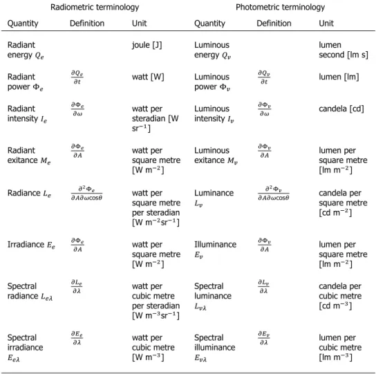
The physics behind nighttime radiation doesn’t differ much from its daytime coun-terpart. There are major differences, however, in what drives the content of the imagery. Compared to the typical daylight situation, there is no uniform light source (i.e. the Sun), which illuminates all objects in a homogeneous manner and would nullify almost all other sources of EM waves in the VNIR part of the spectrum. This leaves room for other light sources to become more apparent, although at lower intensities. Nighttime radiance in the VNIR part of the spectrum is dominated by ar-tificial light sources. With their focus on human vision, it is important to mention the differences between radiometry and photometry. Radiometry is the general field concerned with the measurement of EM waves and their physical quantities [36]. In contrast, photometry additionally takes into account the human perception. Since the human perception is of great importance in the design of artificial light sources, lamp characteristics are predominantly described using photometric terminology. Table 2.1 gives an overview of all relevant radiometric and photometric quantities and units.
2.1.1.
Radiometry
Radiometric quantities describe various aspects of EM radiation, e.g. energy, power and power density with respect to direction and area, or both. Radiant energy 𝑄 is defined by the amount of energy that travels in the form of EM waves, while radiant power or radiant fluxΦ describes the flow of radiant energy over time and is measured in watts (W).
In order to understand the subsequent quantities, first the concept of solid angles needs to be introduced. Essentially, a solid angle Ω defines how large an object seems from a particular viewpoint. In other words, a small object nearby can have the same solid angle as a large object further away. Solid angles are measured in steradian (sr), with 1 sr corresponding to a surface area of 1 square
2
8 2. Background theory
Radiometric terminology Photometric terminology Quantity Definition Unit Quantity Definition Unit Radiant energy joule [J] Luminous energy lumen second [lm s] Radiant power watt [W] Luminous power lumen [lm] Radiant intensity watt per steradian [W sr ] Luminous intensity candela [cd] Radiant exitance watt per square metre [W m ] Luminous exitance lumen per square metre [lm m ] Radiance
cos watt per
square metre per steradian [W m sr ]
Luminance
cos candela per
square metre [cd m ]
Irradiance watt per square metre [W m ]
Illuminance lumen per square metre [lm m ] Spectral radiance watt per cubic metre per steradian [W m sr ] Spectral luminance candela per cubic metre [cd m ] Spectral irradiance watt per cubic metre [W m ] Spectral illuminance lumen per cubic metre [lm m ]
Table 2.1: Radiometric and photometric quantities and units. Note that the photometric unit candela equals lumen per steradian.
metre on a sphere with a radius of 1 metre. Since the total surface of this sphere equals 4𝜋square metres, it follows that the total solid angle about a point is 4𝜋sr. Radiant intensity𝐼, measured in watt per steradian (W sr ), can then be defined as the radiant power from a point source per unit solid angle in the considered direc-tion. Radiant exitance𝑀, in watt per squared metre (W m ), is the radiant power per unit area that leaves a surface. A widely used quantity in remote sensing is that of radiance 𝐿 , defined as the radiant power leaving a surface per unit solid angle and per unit projected area. It is measured in watt per square metre per steradian (W m sr ) and is the preferred quantity for sensor images. Irradiance, on the other hand, is the radiant power received by a surface per unit area, measured in
2.2. Radiation sources
2
9
watt per square metre (W m ). Since most of the above-mentioned quantities are dependent upon wavelength, additional terms, e.g. spectral radiance𝐿 and spectral irradiance𝐿 , are also of importance for the remaining of this thesis. They represent radiance and irradiance, respectively, per unit wavelength.
2.1.2.
Photometry
Photometric quantities, mostly recognised by the prefix luminous, can be derived from their radiometric counterparts using Eq. 2.1. Here Φ represents luminous power (i.e. the photometric quantity),𝐾 is the greatest luminous efficacy which can theoretically be achieved at 555 nm, equalling 683 lm W ,𝑉(𝜆) is the Commis-sion Internationale de l’Eclairage (International CommisCommis-sion on Illumination) (CIE) photopic spectral luminous efficiency or the human eye’s relative sensitivity under well-lit conditions, and Φ represents radiant power (i.e. the radiometric quant-ity). Note thatΦ andΦ can be replaced by any other photometric or radiometric quantity, respectively.
Φ = 𝐾 ∫ 𝑉(𝜆)𝑑Φ (𝜆)
𝑑𝜆 𝑑𝜆 (2.1)
It is important to elaborate here on the difference between photopic, scotopic and mesopic vision. Photopic vision is the standard in normal well-lit conditions where the luminance exceeds 3 cd m . Under these circumstances, human vision is dominated by the eye’s cones, which are good at discriminating different colours. Scotopic vision, on the other hand, is dominated by rods. These rods are more sensitive to light, but are less efficient at discriminating colours, and are, therefore, very effective in low light conditions (i.e. below 0.003 cd m ). Whereas the highest sensitivity of photopic vision is centred around 555 nm, scotopic vision has its peak around 507 nm (Fig. 2.1). For intermediate luminances, both cones and rods are used, a state called mesopic vision. Since luminances as a result of artificial lighting usually approximate the values for photopic vision, the spectral luminous efficiency curve for photopic vision is frequently used in lighting design.
2.2.
Radiation sources
So far, the identification of light source types and intensities from aerial or space-borne imagery has been challenging due to a limited spatial and spectral resolution. While it is possible to give an extensive overview of the different sources of radi-ation in the VNIR part of the spectrum, relative worldwide frequencies are difficult to determine. Instead, most research has focused on associating the amount of reflected light with land use classes. One such example is the aerial campaign ex-ecuted by Kuechly et al. [30] for the city of Berlin. After a thorough analysis of light emission, streets were found to be responsible for 31.6% of the total light emitted, although only covering an area of 13.6%. Other large contributions were coming from industrial areas (15.6%), public service areas (9.6%), block buildings (7.8%) and the city centre (6.3%). The concentration of nighttime radiation around the major transportation axes (Fig. 2.2) hints at the fact that nocturnal light is mostly
2
10 2. Background theory
Figure 2.1: CIE photopic (purple) and scotopic (orange) spectral luminous efficiency curves, represent-ing the sensitivity of the human eye to different wavelengths under well-lit and low-light conditions, respectively. Note the bell-shaped forms centred around 555 nm and 507 nm.
restricted to urban areas, in contrast to rural regions. Even though these outcomes do not tell anything on lighting types directly, it shows that artificial lights are the dominant emission sources.
2.2.1.
Artificial lights
The sources used by humans to produce lighting have changed drastically through-out history, going from open fires to candles and oil lamps over natural gas to electrical light. An estimate made by the Joint Research Centre of the European Commission [37] shows that, among artificial light sources, high-pressure sodium lights were responsible for about half of the artificial light in the European Union in 2015, although a trend towards the use of LED lights is to be expected in the near future. Below follows an overview of the most common exterior lighting types used today and a description of their principal emission peaks, i.e. those wavelengths for which a particular light emits most of its light.
Incandescent
The incandescent lamp emits light by heating a tungsten filament inside a vacuum enclosed by a glass bulb. When electricity passes through the filament, it heats up, thereby producing a spectrum similar to that of a blackbody of the same temperat-ure. However, these bulbs come with a major shortcoming, as most of the emitted light falls in the infrared part of the spectrum (Fig. 2.3c). Emission for incandescent light bulbs usually peaks around 1000 nm.
High- and low-pressure sodium
High- and low-pressure sodium lamps are a type of gas discharge lamp which use sodium in an excited state. Gas discharge lamps generate radiation by sending electricity through an ionised gas, thereby releasing energy in the form of photons. Different gasses typically result in their own characteristic emission lines. In the case of high-pressure sodium lamps, the strongest is at 819 nm (Fig. 2.3d). Sec-ondary lines lie between 560 nm and 620 nm. Low-pressure sodium lamps have
2.2. Radiation sources
2
11
Figure 2.2: Nighttime image of Berlin, Germany, September 11, 2010. Reprinted from ”Aerial survey and spatial analysis of sources of light pollution in Berlin, Germany,” by H.U. Kuechly, C.C.M. Kyba, T. Ruhtz, C. Lindemann, C. Wolter, J. Fischer and F. Hölker, 2012,Remote Sensing of Environment, 126,
p. 44.
an additional outer vacuum surrounded by glass covered with an infrared reflected layer. This limits the emission of infrared light, leaving only a strong emission peak at 589 nm (Fig. 2.3e). Sodium vapour lamps typically emit a bright yellow-orange light.
Mercury vapour
Mercury vapour lamps are another type of gas discharge lamps, using mercury and providing a more blue-green color because of its peak emissions between 540 nm and 580 nm (Fig. 2.3f). In contrast to other discharge lamps, it addition-ally resembles the curve of an incandescent lamp, with a blackbody peak around 1250 nm [34].
Metal halide
Metal halide lamps are similar to mercury vapour lamps, but with an additional mixture of metal halides added to the mercury. Metal halide lamps generally have a strong peak at 819 nm, with other peaks strongly depending on the composition of the halides [34] (Fig. 2.3g).
Fluorescent
Fluorescent lamps are low-pressure gas discharge lamps using fluorescence to pro-duce radiation. Like with mercury vapour lamps, they make use of mercury gas. However, the inner surface of the glass tube in which the gas resides contains a fluorescent coating of phosphors. This results in two main emission peaks at 544 nm
2
12 2. Background theory
Figure 2.3: Typical emission spectra for different nighttime radiation sources: (a) full moon; (b) fire, 700 K; (c) incandescent bulb; (d) high-pressure sodium lamp; (e) low-pressure sodium lamp; (f) mercury vapour lamp; (g) metal halide lamp; (h) fluorescent lamp; (i) warm LED lamp; and (j) cool LED lamp [34]. Note that the y-axis represents relative radiances.
2.2. Radiation sources
2
13
and 611 nm (Fig. 2.3h). Near-infrared emission are smaller than for mercury vapour lamps.
Light emitting diodes
LED lamps consist of one or more LEDs, which are semi-conductors with electrons moving to a lower energy state when electrical current runs through it, thereby releasing photons. Different types of semi-conductors can be used to create a wide range of colours. Therefore, it is difficult to pinpoint specific emission peaks for LED lamps. They can, however, be identified by relatively narrow symmetrically shaped emission bands and a lack of near-infrared emissions [34]. White LEDs generally have two primary peaks, i.e. one in the blue and another one in the green to red region (Fig. 2.3i-j). Because of their long lifespan and high efficiency, LED lights are becoming more and more the standard for both indoor and outdoor lighting.
2.2.2.
Moon
Apart from the artificial light sources mentioned above, there are in fact a num-ber of natural light sources emitting light in the visible part of the spectrum during nighttime. The most prominent of those is the Moon, reflecting sunlight arriving at its surface onto Earth. Hence, the Moon is actually not a light source in itself, but instead acts as a reflecting object. The intensity of moonlight is rather small in comparison to direct sunlight or artificial lighting (see Table 2.2 for comparison). In contrast to artificial lighting, however, the emitted light is not focused, but instead homogeneous across the surface. Therefore, moonlight can become significant, even though its intensity is relatively limited. Additionally, moonlight is crucial in the detection of clouds from DMSP or VIIRS imagery. It also explains the relat-ively low detection limits of both of these sensors, as their principal focus is on cloud detection. Additionally, moonlight facilitates the possibility to observe snow and ice features from space [38]. Compared to the spectrum of artificial lighting, lunar spectral irradiances are relatively homogeneous across the VNIR spectrum (Fig. 2.3a).
2.2.3.
Other
Another relatively common source of nighttime radiation is that caused by fires. Fire emission spectra (Fig. 2.3b) can be described using Planck’s law for blackbodies:
𝐿 = 2ℎ𝑐 𝜆
1
𝑒 / − 1, (2.2)
where 𝐿 represents the spectral radiance, ℎ denotes Planck’s constant, 𝑐 is the speed of light,𝑘 is Boltzmann’s constant and𝑇is the absolute temperature of the material. For typical fires with temperatures ranging between 400 K and 1200 K, emission peaks are located in the thermal infrared part of the spectrum. Other sources, usually less frequent or at lower intensities, include lightning, auroras, gas flares, luminous bacteria and dinoflagellates (i.e. bioluminescence), and sky-glow [2] (Fig. 2.4). As the focus is on urban areas, however, the latter sources are not considered during the remainder of this thesis.
2
14 2. Background theory
Figure 2.4: Conceptual diagram of observable features at night under different conditions, with (a) full moon conditions; and (b) new moon conditions. Courtesy of Steven Dayo, University Corporation for Atmospheric Research COMET program [39].
2.3. Lighting quality parameters
2
15 Situation Illuminance [lm m ] Full sunlight 103 000 Partly sunny 50 000 Cloudy day 1 000 - 10 000 Main road street lighting 15Lighted parking lot 10 Residential side street 5 Urban skyglow 0.15 Full moon, cloud-free 0.1 - 0.3 Quarter moon 0.01 - 0.03 Clear starry night 0.001
Overcast night sky 0.00003 - 0.0001
Table 2.2: Typical illuminance values for different situations. Reprinted from ”The ecological impacts of nighttime light pollution: a mechanistic appraisal,” by K.J. Gaston, J. Bennie, T.W. Davies and J. Hopkins, 2013,Biological Reviews, 88(4), p. 913.
2.3.
Lighting quality parameters
As it is not effective to share full lamp spectra with consumers, the technical de-scription of artificial lighting generally consists of only a limited number of perform-ance parameters or indices. These define, e.g., how much of the full spectrum can be seen by the human eye, or how much light is emitted in the blue part of the spectrum. Below, the most common spectral indices in lighting engineering are discussed, based on a recent report on road lighting and traffic signals by the Joint Research Centre of the European Commission, put together by researchers and some of the industry’s stakeholders [37].
2.3.1.
Radiant power
The first light parameter that plays an important role is the intensity or radiant power that corresponds to a certain luminaire system. Its estimation from satellite images, however, is not straightforward, as it depends on a number of different parameters, e.g. surface reflection, atmospheric transmittance and the ratio of emitted power within the measured spectrum. Whereas it is possible to estimate radiant power of lamps, uncertainties remain relatively high, e.g. because of missing aerosol data at high spatial resolutions [40]. Usually, rather than the radiant power, it is the required electrical power that is of interest. However, estimating the latter is further
2
16 2. Background theory
complicated by the need for data on electrical power efficacy, which describes the ability to transform electrical power into optical power, and the amount of lamp shielding. Advances in this area requires additional research, but remains outside the scope of this thesis. Moreover, such estimations do not depend on the choice of spectral bands and will, therefore, not be discussed further here.
2.3.2.
Luminous efficacy
In designing artificial lighting, achieving a high luminous efficacy (LE) is crucial. Lu-minous efficacy rates the amount of visible light that is produced, in lumen, divided by the total amount electrical power that is required. Therefore, it is a measure for the efficiency of a particular luminaire system. Not only does LE take into account emissions outside of the visual spectrum, but also power losses in control gear or a decreased lumen output as a result of dirt collection on the luminaire. As LE is usually difficult to estimate without any ground-based information, it is often inter-changed with luminous efficacy of radiance (LER), which can be computed as the ratio between luminous powerΦ and optical radiant powerΦ (Eq. 2.3). Typical LE values for road lighting range from 50 lm W for mercury lamps, through 80 lm W for fluorescent lamps and 100-140 lm W for LED lamps, to 140-170 lm W for low-pressure sodium lamps [37]. Values of over 200 lm W are expected for future LED road lighting.
𝐿𝐸𝑅 = Φ Φ =
𝐾 ∫ 𝑉(𝜆) ( )𝑑𝜆
∫ ( )𝑑𝜆 (2.3)
2.3.3.
Spectral G index
Light pollution, especially in the blue part of the spectrum, has gained substantial attention in recent years. Well-known examples are the disruptive effect of arti-ficial lights on the nocturnal behaviour of different species, as well as on human health [6, 7]. For a long time, CCT has been the principal indicator for the amount of emitted blue light, despite its inability to sufficiently describe a lamp’s spectrum (see Section 2.3.4). Recently, however, the European Commission’s Joint Research Centre has published a report in which it recommends the use of the so-called C(L500,V) or spectral G index instead [37]. This index can be computed as the total amount of luminous power divided by the amount of radiant power emitted between 380 nm and 500 nm (Eq. 2.4), with high values corresponding to low blue light emissions [41]. Note the similarities between the enumerator of this equation and the one of Eq. 2.3. This means that, later on, the enumerator can be estimated by the same spectral band. With most of modern streetlights being non-Planckian radiators, for the remainder of this thesis, more emphasis will be placed on the estimation of the spectral G index, as opposed to estimating CCT.
𝐺 = 2.5log ∫ 𝑉(𝜆)
( )
𝑑𝜆
2.3. Lighting quality parameters
2
17
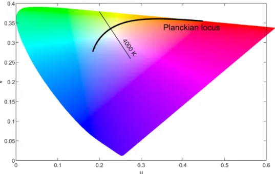
Figure 2.5: CIE 1960 colour space, with the Planckian locus line representing ideal blackbody radiators. The isotherm perpendicular to the Planckian locus represents all positions in the CIE 1960 colour space with a correlated colour temperature of 4000 K.
2.3.4.
Correlated colour temperature
In order to assess the perceived colour of the light emitted by a particular lamp, its spectrum is compared to a range of blackbody radiators, which follow Planck’s law (Eq. 2.2). The absolute temperature of the blackbody that most closely re-sembles the spectrum of the lamp, defines the so-called correlated colour temper-ature (CCT). It needs to be noted that, while the computation of CCT values is relevant for lamps that closely resemble the spectrum of a Planckian source, e.g. in the case of incandescent lamps, it is no longer relevant for other lighting technolo-gies such as discharge lamps or LED lamps. Despite its limited ability to describe a lamps’ spectrum, CCT remains a widely applied indicator, as it is relatively straight-forward to grasp its meaning.
The computation of the CCT value of a lamp is based on its spectral power dis-tribution, which can in this case be exchanged by its irradiance spectrum𝐸 , [42].
In a first step, the so-called tristimulus values 𝑋, 𝑌 and 𝑍 are computed using Eq. 2.5-2.7. Here, ̄𝑥, ̄𝑦and ̄𝑧represent the CIE’s color-matching functions, as given by the CIE. Note that 𝐾 is chosen, in order for𝑌 to equal 100. In the next step, the chromaticity coordinates 𝑥and 𝑦in the CIE 1931 coordinate system are com-puted (Eq. 2.8-2.9). From these, the chromaticity values 𝑢and𝑣 in the CIE 1960 UCS diagram need to be computed (Eq. 2.10-2.11). Within this diagram (Fig. 2.5), the Planckian radiator whose coordinates are nearest to the computed chromaticity values𝑢and𝑣, determines the temperature, and hence the CCT of the lamp.
2
18 2. Background theory 𝑋 = 𝐾 ⋅ ∫ ̄𝑥 ⋅ 𝐸, ⋅ 𝑑𝜆 (2.5) 𝑌 = 𝐾 ⋅ ∫ ̄𝑦 ⋅ 𝐸, ⋅ 𝑑𝜆 (2.6) 𝑍 = 𝐾 ⋅ ∫ ̄𝑧 ⋅ 𝐸, ⋅ 𝑑𝜆 (2.7) 𝑥 = 𝑋 𝑋 + 𝑌 + 𝑍 (2.8) 𝑦 = 𝑌 𝑋 + 𝑌 + 𝑍 (2.9) 𝑢 = 4𝑥 −2𝑥 + 12𝑦 + 3 (2.10) 𝑣 = 6𝑦 −2𝑥 + 12𝑦 + 3 (2.11)Another frequently cited parameter to describe a light source’s spectrum is that of the colour rendering index (CRI), which expresses a lamp’s ability to faithfully reproduce different colours along the spectrum, compared to a blackbody radiator with the same CCT. Typically, incandescent lamps have high CRI values close to the maximum value of 100. Low-pressure sodium lights, on the other hand, have only one narrow peak in its spectrum and, therefore, yield low CRI values, near 0. As has been expressed before by Elvidge et al. [34], estimating CRI requires a very high spectral resolution, which is not cost-effective for current nighttime satellite sensors. As a consequence, the estimation of CRI will not be considered in this thesis.
2.4.
Propagation of electromagnetic radiation
In optical radiation, light is modelled as transverse sinusoidal waves, which oscillate electric and magnetic fields perpendicular to the direction of propagation. Hence, they are called electromagnetic (EM) waves. The intensity of radiation that can be measured is encoded in the amplitude of these waves. Once leaving a light source, such EM waves travel to the Earth’s surface, interact with the surface or any other object and travel through a whole series of atmospheric layers up to the sensor. When EM waves interact with matter, the electrons, molecules and/or nuclei are put into motion, thereby transferring energy from the wave to the object [43]. Below, the interaction of waves with materials is subdivided into two sections, namely the energy interaction with the Earth’s surface (Section 2.4.2) and energy interactions in the atmosphere (Section 2.4.3).
2.4. Propagation of electromagnetic radiation
2
19
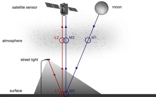
Figure 2.6: Simplified illustration of propagation of nighttime radiation in optical remote sensing, with (L1) surface interaction with lamp EM waves; (L2) upward atmosphere interaction with lamp EM waves; (M1) downward atmosphere interaction with lunar EM waves; (M2) surface interaction with lunar EM waves; and (M3) upward atmosphere interaction with lunar EM waves. Note that only cloud-free condi-tions are considered.
2.4.1.
Pathway
Figure 2.6 represents a simplified illustration of the path of EM waves under cloud-free nighttime conditions. The model consists of two fundamental light sources, i.e. artificial lights or street lights (prefix L) and the Moon (prefix M). Note that, although it is strictly not a light source, the Moon is considered as one for ease of computa-tion. Lunar radiation, a result of reflected sunlight, passes through the Earth’s atmo-sphere twice, as is the case for sunlight in daytime optical remote sensing. Artificial light sources, on the other hand, are usually relatively close to the Earth’s surface. Therefore, it can be assumed that only upward paths are of importance, restricting the atmospheric transmission problem to a conversion from bottom-of-atmosphere (BOA) radiances to top-of-atmosphere (TOA) radiances. Contrary to the presented diagram (Fig. 2.6), it needs to be noted that real-world environments are much more complex, since waves can be scattered, absorbed or reflected multiple times, the Earth’s atmosphere is not a homogeneous or static environment, the cloud-free assumption usually doesn’t hold and path radiance or adjacency effect are not con-sidered. For the determination of optimal spectral and spatial resolutions, however, a simplified model of EM wave propagation is sufficient.
2
20 2. Background theory
2.4.2.
Surface interaction
When incident EM waves come into contact with the Earth’s surface, their energy may be absorbed, transmitted or reflected. The proportion of each of these energy interactions strongly depends on both wavelength and material characteristics. For example, two different materials (e.g. grass and asphalt) look different in a satel-lite image as a result of different material properties. Similarly, a patch of grass reflects a different amount of red light compared to green light. A widely used char-acteristic of surface features is spectral reflectance, which measures the amount of reflected energy with respect to the amount of incident energy as a function of the wavelength.
Another important consideration is the direction in which incoming energy is reflected. This depends mostly on the roughness of the object, where specular reflectors and diffuse reflectors can be distinguished. Specular reflectors are flat surfaces that result in mirror-like reflections. In other words, light is reflected in a single direction, with the reflection angle equalling the incidence angle. Diffuse or Lambertian reflectors, on the other hand, are rough surfaces that reflect uniformly in all directions. Most real-world surfaces or objects are neither perfectly specular nor perfectly Lambertian and are a combination of both. Therefore, it is obvious that spectral reflectance curves do not fully grasp the complexity of surface interaction, as they usually don’t take the incidence angle of incoming light and the viewing angle into consideration. For this reason, the bidirectional reflectance distribution function (BRDF) was introduced (Eq. 2.12), with𝑓 representing the BRDF, 𝐿 the reflected radiance, 𝐸 the incoming irradiance, 𝜙 and 𝜃 the azimuth and zenith angle of the reflected radiance, respectively, and 𝜙 and𝜃 the azimuth and zenith angle of incoming light. As radiance is measured in W m sr and irradiance in W m , the BRDF has the unit sr .
𝑓 = 𝑑𝐿 (𝜙 , 𝜃 )
𝑑𝐸 (𝜙 , 𝜃 ) (2.12)
Deriving BRDF values from spaceborne or airborne sensors, however, is not straightforward. Instead, the assumption that all surface objects are perfect Lam-bertian reflectors is applied in most cases. In other words, the incoming light is assumed to reflect equally in all directions and the direction from which the light is coming is of no importance. This allows for the complex BRDF to be replaced by the rather uncomplicated determination of spectral reflectance. It has to be noted, however, that this simplification does not always stroke with reality. One such case is the example of a wet road surface, which closely resembles a purely specular re-flector. As the presence of wet road surfaces is highly correlated with the presence of clouds, and only cloud-free optical imagery are taken into account, this effect has only limited implications and can, thus, be neglected.
2.4.3.
Atmosphere interaction
After interacting with the surface and assuming there is no path radiance, the re-flected EM waves continue on their path to the sensor through different layers of the atmosphere, i.e. troposphere, stratosphere, mesosphere, thermosphere and
exo-2.4. Propagation of electromagnetic radiation
2
21
Figure 2.7: Variation in atmospheric transmission curves for a mid-latitude summer atmosphere with urban aerosol model at sea level.
sphere. Here, three fundamental interactions can occur: transmission, absorption and scattering. Whereas scattering changes the direction of the waves, absorption and transmission determine the amount of energy that passes through the atmo-sphere. Various molecules, such as water vapour, carbon dioxide and ozone, can absorb EM energy and convert it into other forms of energy. As a consequence, the energy does no longer reach the sensor and information is lost. Different con-stituents absorb energy of different wavelengths. Their cumulative effect causes the atmosphere to become almost completely impenetrable in certain wavelength ranges (Fig. 2.7). Absorption can vary strongly for different atmospheric conditions. For example, the amount of water vapour above the tropics is significantly larger than the amount above the poles. Hence, for wavelengths prone to absorption by water vapour, transmission will be lower above tropical regions.
Atmospheric scattering, or diffusion of radiation by atmospheric particles, can severely reduce the information content of remote sensing data as EM waves are redirected from their original path. This leads to an uncertain origin of the sensed radiation. Three different types of scattering take place, i.e. Rayleigh scattering, Mie scattering and non-selective scattering. Rayleigh scattering is dominant when atmospheric particles interact with waves that have a wavelength much larger than the size of the particle. Such particles include tiny dust specks, nitrogen and oxy-gen. Shorter wavelengths are more affected by Rayleigh scattering than longer wavelengths, as the effect is inversely proportional to the wavelength. This causes RGB satellite images to look blue when taken from a high altitude. Additionally, it reduces the contrast of spaceborne images. When the size of the particles is similar to the wavelength (e.g. pollen, dust or smog), Mie scattering occurs. In contrast to Rayleigh scatter, Mie scatter affects more the wavelengths from near-ultraviolet to mid-infrared and is especially significant during overcast conditions. In such con-ditions, it produces a general haze in the image. Lastly, non-selective scattering comes about when the particles are much larger than the wavelength, as is the case, e.g., for water droplets in clouds. As non-selective scattering is independent of the wavelength in the VNIR part of the spectrum, with equal quantities of blue, green, red and near-infrared light scattered, clouds appear white in VNIR images.
2
22 2. Background theory
2.5.
Optical imaging system
2.5.1.
Spectral sampling
Optical systems have the purpose of producing a radiance image on the focal plane array of an imaging system from incoming EM waves. In the case of multi-spectral imaging, it does so in different spectral bands, with each band sensitive to a par-ticular range of wavelengths. This can be seen as a form of spectral sampling, with the smallest difference in wavelengths that can be distinguished, to be inter-preted as its spectral resolution. To compute the signal that arrives at a sensor, through combining radiances from different wavelengths, there are two options, i.e. the band-integrated radiance and the band-averaged spectral radiance. The band-integrated radiance𝐿 , defined as the peak normalised effective radiance value over the detector bandpass, can be computed by applying
𝐿 = ∫ 𝐿 ⋅ 𝑅 , ⋅ 𝑑𝜆, (2.13)
where𝐿 represents the spectral radiance and𝑅 , is the instrumental spectral
response function or slit function for a given band [44]. It is measured in W m sr . The band-averaged spectral radiance 𝐿 , , on the other hand, is the weighted
average of the normalised effective radiance value over the detector bandpass (Eq. 2.14) and is measured in W m sr nm . As the band-averaged spec-tral radiance is better at comparing radiance values across different bands, it is generally the preferred variable.
𝐿 , =
∫ 𝐿 ⋅ 𝑅 , ⋅ 𝑑𝜆 ∫ 𝑅, ⋅ 𝑑𝜆
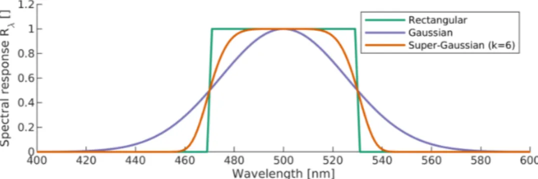
(2.14) Slit functions are difficult to be synthesised accurately beforehand. As a general rule, however, such filters are described by an analytical function which behaves as a combination of a rectangular function and a Gaussian function. Commonly, a so-called symmetric ’super-Gaussian’ function of the form
𝑅 = 2 | | (2.15)
is used, where𝜆 represents the central wavelength (CW) of the band,Δ𝜆is the full width at half maximum (FWHM) or bandwidth and 𝑘 denotes a parameter which defines the shape of the function [45]. For high𝑘values, the function resembles a rectangular function, while for𝑘 values close to 2 the Gaussian function is approx-imated. For optical remote sensing purposes, 𝑘 = 6 usually results in realistic slit functions (Fig. 2.8) [46].
2.5.2.
Noise model
The signal that constitutes an optical satellite image does not only contain radi-ances originating from the light sources mentioned in Section 2.2. Additionally, it might include background radiances from sunlit objects in the case of relatively
2.5. Optical imaging system
2
23
Figure 2.8: Different analytic slit functions for a band with a central wavelength of 500 nm and an FWHM of 60 nm.
low solar zenith angles, stray light in case the satellite is directly lit by sunlight, and high energy particles. Moreover, noise can be introduced during the charge transfer process caused by detectors and electronic devices. Here, the focus lies on radiometric or system noise because other noise sources, such as straylight, are relatively straightforward to model. To compare the amount of desired signal power to the level of background noise, signal-to-noise ratio (SNR) is defined as
𝑆𝑁𝑅 =𝑁
𝑁 , (2.16)
where𝑁 and𝑁 are the signal electron number and noise electron number, respectively. The largest radiometric noise contribution is a result of the random incidence of photons, thereby randomly generating photo-generated electrons. This type of noise is called photon shot noise 𝜎 , measured in electron number. Assuming photon shot noise to be dominant and other contributions negligible, the noise electron number can be rewritten as the square root of the signal electron number (Eq. 2.17), thereby obeying a Poisson distribution [47]. The signal electron number𝑁 itself can be found by converting the incoming spectral radiance to electron content (Eq. 3.2), with𝐴being the detector’s effective area, equalling the pixel area times the pixel’s fill factor, 𝜏 is the system’s optical transmittance, 𝜂 is the quantum efficiency,𝑡is the integration time,𝑓/#is the f-number,ℎis Planck’s constant and𝑐is the speed of light [48]. Typical sensor values for a nighttime VNIR sensor are given in Table 2.3.
𝑁 ≈ 𝜎 = √𝑁 (2.17)
𝑁 = 𝐿 , ⋅ 𝐴 ⋅ 𝜋 ⋅ 𝜏 ⋅ 𝜂 ⋅ 𝑡 ⋅ Δ𝜆 ⋅ 𝜆
(4(𝑓/#) + 1) ⋅ ℎ ⋅ 𝑐 (2.18) The so-called noise-equivalent radiance (NER), i.e. the amount of noise meas-ured in W m sr nm , can then be defined as
2
24 2. Background theory 𝑁𝐸𝑅 = 𝑁 ⋅ (4(𝑓/#) + 1) ⋅ ℎ ⋅ 𝑐 𝐴 ⋅ 𝜋 ⋅ 𝜏 ⋅ 𝜂 ⋅ 𝑡 ⋅ Δ𝜆 ⋅ 𝜆 ≈ √𝐿 , ⋅ 𝐴 ⋅ 𝜋 ⋅ 𝜏 ⋅ 𝜂 ⋅ 𝑡 ⋅ Δ𝜆 ⋅ 𝜆 (4(𝑓/#) + 1) ⋅ ℎ ⋅ 𝑐 ⋅ (4(𝑓/#) + 1) ⋅ ℎ ⋅ 𝑐 𝐴 ⋅ 𝜋 ⋅ 𝜏 ⋅ 𝜂 ⋅ 𝑡 ⋅ Δ𝜆 ⋅ 𝜆 = √𝐿 , ⋅ (4(𝑓/#) + 1) ⋅ ℎ ⋅ 𝑐 Δ𝜆 ⋅ 𝜆 ⋅ 𝐴 ⋅ 𝜋 ⋅ 𝜏 ⋅ 𝜂 ⋅ 𝑡 (2.19)meaning that the NER depends on the square root of the band-averaged spectral radiance𝐿 , , and on the inverse square root of both the FWHMΔ𝜆and CW𝜆 .
2.5.3.
Radiometric sampling
Assuming detectors have a linear response, the conversion from an incoming band-averaged spectral radiance𝐿 , to a digital number (DN) is computed using
𝐷𝑁 = (𝐿 , − 𝑏) ⋅ 𝑐 , (2.20)
where
𝑏 = 𝐿 , 𝑐 =𝐿 − 𝐿
𝐷𝑁 , (2.21)
with 𝑏 and 𝑐 denoting the offset and gain of the system, respectively. 𝐿 and 𝐿 represent the detection limit and the saturation of the sensor, while𝐷𝑁 is the maximum digital number that can be attained (e.g. 255 for 8 bit images). The radiometric resolution of a sensor system can be defined as both the amount of bits that is used for storage, as well as the radiance which corresponds to a single DN.
2.5.4.
Spatial sampling
Similar to the spectral and radiometric cases, spatial resolution can be seen as a form of sampling, i.e. a form of sampling of the ground surface. Primarily, the definition of ground sample distance (GSD) is used, which defines the distance at the surface between two adjacent pixel centres. This metric does not, however, ne-cessarily act as an accurate surrogate for spatial resolution. For example, an image can be spatially oversampled and contain closely spaced, but blurry pixels. There-fore, ground resolved distance (GRD) should be considered additionally. It defines the geometric size of the smallest object which can be detected by a sensor [48]. This measure depends heavily on the so-called point spread function (PSF) of a sensor, which characterises its response to a point source. Based on the definition of PSF, the instantaneous field of view (IFOV) can be interpreted as the angle 𝛼 between specified cutoff levels of the PSF. The GRD, then, represents the geometric projection of this IFOV on the ground surface. With most remote sensing systems designing the pixel spacing (i.e. GSD) closely resembling the GRD, both can usually be interchanged without much issues.
2.6. Physically-based rendering
2
25
Variable Value
Band-averaged spectral radiance 250 W m sr Pixel pitch 7⋅10 m Pixel fill factor 0.95
Effective area 4.66⋅10 m Optical transmittance 0.8
Quantum efficiency 0.85 Integration time 2.2⋅10 s Time delayed integration 256 Effective integration time 5.63⋅10 s Bandwidth 100⋅10 m Central wavelength 560⋅10 m
F-number 2.5
Projected solid angle 1.21⋅10 sr Planck’s constant 6.63⋅10 W s Speed of light 3.00⋅10 m s
Signal 160 e
Photon shot noise 12.6 e
Table 2.3: Example computation of signal electron content and photon shot noise for a typical nighttime situation, based on Elvidge et al. [17] and IMEC’s CCD-in-CMOS multispectral sensor [49].
2.6.
Physically-based rendering
Rendering is a part of computer graphics that deals with generating, or render-ing, a two-dimensional image from a textual description of, e.g., a virtual camera, three-dimensional objects and light sources [50]. The appearance of the objects in the final image is determined by different characteristics, including material prop-erties, textures and shading properties. The field of rendering is especially popular in product design, architecture, advertising, computer games and movies. As a subfield of rendering, physically-based rendering focuses on accurately resembling the propagation of light as it takes place in reality. Its ultimate goal is to generate an image that is indistinguishable from a photograph of the same scene.
There-2
26 2. Background theory
fore, physically-based rendering is the fitting tool for generating realistic nighttime satellite imagery at high spatial and spectral resolutions. In this thesis, Persistence of Vision Raytracer (POV-Ray) is the rendering software of choice. For a full de-scription of the software and its possibilities, readers are referred to the POV-Ray manual [51].
2.6.1.
Rendering equation
The rendering equation (Eq. 2.22) forms the foundation of physically-based render-ing and global illumination algorithms [52]. In essence, it illustrates the transport of light using a recursive integral equation. It describes, in other words, the total amount of outgoing radiance𝐿 from a pointp along a viewing directionv, given a function for the incoming radiance 𝐿 (Eq. 2.23) and a BRDF𝑓(l,v). Here, 𝐿 represents the emitted radiance from a surface at point p, lis the incoming dir-ection, Ωthe hemisphere of directions abovep, (n⋅l) the dot product betweenn
andlwith negative values replaced by zero, and𝑟(p,l) a ray tracing function which returns the location of the first surface point which is hit by a traced ray from p
in direction l. Essentially, Equation 2.23 means that the radiance coming into a point palong directionlis equal to the radiance going out from some other point in the opposite direction -l. Hence, it is a recursive term computed ad infinitum. Algorithms, therefore, need some kind of stopping conditions. An important prop-erty of the rendering equation is its linearity with respect to the emitted radiation. It is linear in the sense that if a certain light source becomes twice as strong, the lit object’s radiance will have doubled as well.
𝐿 (p,v) = 𝐿 (p,v) + ∫
l∈
𝑓(l,v)𝐿 (p,l)(n⋅l) 𝑑l (2.22)
𝐿 (p,l) = 𝐿 (𝑟(p,l), −l) (2.23) Solving the full rendering equation, however, is not a simple task. Algorithms that solve it can create extremely photorealistic images. At the same time, they are also computationally very expensive. Two of the most common ways of solving the rendering equation are finite element methods (e.g. the radiosity method) and Monte Carlo methods (e.g. the ray tracing method). POV-Ray has the possibility to use a combination of both approaches. Below, the two approaches are briefly described.
2.6.2.
Ray tracing
Ray tracing is the most widely used Monte Carlo technique used for solving the ren-dering equation. In general, Monte Carlo integration schemes use random numbers in order to evaluate integrals, with the expected value exactly equalling the value of the integral. As is the case with Monte Carlo techniques, a physically correct image can thus be generated as long as the algorithm runs for a long enough time. As the name implies, ray tracing uses the tracing of rays to determine the transportation of light between different scene elements. However, in contrast to the direction of light waves in the real world, ray tracing is done backwards. This means that rays