On Bayesian Methods in Network Regression

(1)

UC Santa Cruz

UC Santa Cruz Electronic Theses and Dissertations

Title

Permalink

https://escholarship.org/uc/item/12z7c13k

Author

Guha, Sharmistha

Publication Date

2019 Peer reviewed|Thesis/dissertation

(2)

UNIVERSITY OF CALIFORNIA SANTA CRUZ

ON BAYESIAN METHODS IN NETWORK REGRESSION

A dissertation submitted in partial satisfaction of the requirements for the degree of

DOCTOR OF PHILOSOPHY in STATISTICAL SCIENCE by Sharmistha Guha December 2019

The Dissertation of Sharmistha Guha is approved:

Professor Abel Rodriguez, Chair

Professor Athanasios Kottas

Professor Herbert Lee

Quentin Williams

(3)

Copyright cby

Sharmistha Guha 2019

(4)

List of Figures

2.1 Posterior probability that a node is influential,P(ξk =1|Data), for each node

and each of the 11 cases associated withSimulation 1. Dark cells correspond to the truly influential nodes. . . 33

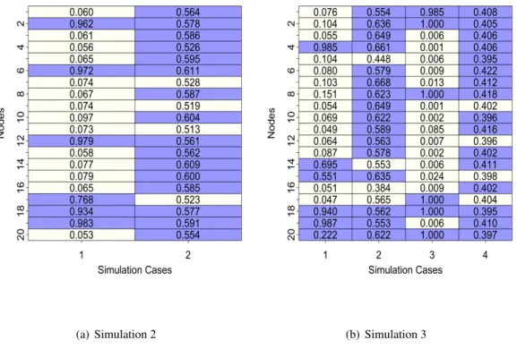
2.2 Posterior probability that a node is influential,P(ξk =1|Data), for each node

and all cases associated withSimulation 2andSimulation 3. Dark cells corre-spond to the truly influential nodes.. . . 34

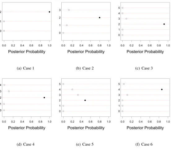
2.3 Posterior probability distributions of the effective dimensionality in cases 1−6 inSimulation 1. Filled bullets indicate the true value of effective dimensionality. 38

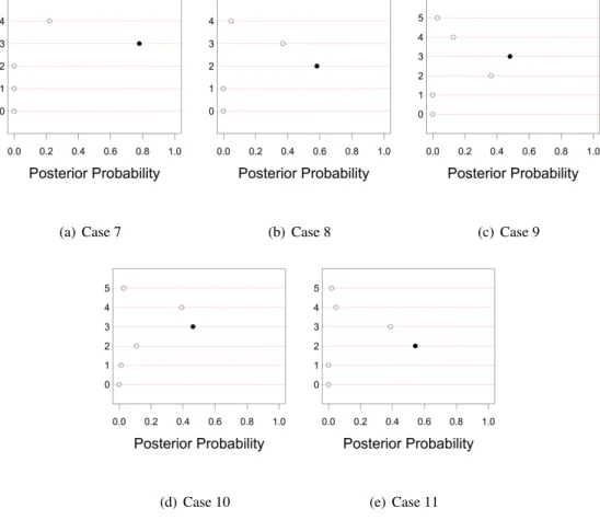
2.4 Posterior probability distributions of the effective dimensionality in cases 7−11 inSimulation 1. Filled bullets indicate the true value of effective dimensionality. 39

2.5 Maps of the brain network (weighted adjacency matrices) for two representative individuals in the sample. Since the(k,l)-th off-diagonal entry in any adjacency matrix corresponds to the number of fibers connecting the k-th and the l-th ROIs, the adjacency matrices are symmetric. Hence the figure only shows the upper triangular portion. . . 48

(8)

2.6 Posterior means of the latent positionsu1, . . . ,uV for the two highest-variance

components of the latent space. . . 49

2.7 Significant connections detected among influential brain regions of inter-est (ROIs) in the Desikan atlas. White cells show significant nodal associations among ROIs. Prefix ‘lh-’ and ‘rh-’ in the ROI names denote their positions in the left and right hemispheres of the brain respectively. . . 53

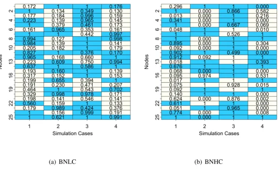
3.1 Simulation 1: clear background denotesuninfluentialand dark background de-notes influential nodes in the truth for BNLC and BNHC models. Note that there are 25 rows (corresponding to 25 nodes) and 4 columns corresponding to 4 different cases in Simulation 1. The model-detected posterior probability of being influential has been super-imposed onto the corresponding node. . . 72

3.2 Simulation 2: clear background denotesuninfluentialand dark background de-notes influential nodes in the truth for BNLC and BNHC models. Note that there are 25 rows (corresponding to 25 nodes) and 4 columns corresponding to 4 different cases in Simulation 2. The model-detected posterior probability of being influential has been super-imposed onto the corresponding node. . . 73

3.3 Figure shows classification performance in the form of Area under Curve (AUC) of ROC for all cases in Simulations 1 and 2. . . 77

3.4 Plots showing posterior probability distribution of effective dimensionality for BNLC and BNHC models in all 4 cases in Simulation 1. Filled bullets indicate the true value of effective dimensionality. . . 78

(9)

3.5 Plots showing posterior probability distribution of effective dimensionality for BNLC and BNHC models in all 4 cases in Simulation 2. Filled bullets indicate the true value of effective dimensionality. . . 79

3.6 Figure shows P(ξk =1|Data) for BNLC and BNHC under different

hyper-parameter combinations in the simulated data for case 4 (Simulation 1). . . 82

3.7 Figure shows the posterior probabilities of nodes selected asinfluentialby one method, but not by another, of being active. . . 87

3.8 Lateral and medial views of the brain (left and right hemispheres) showing all 68 regions of interest (ROIs). The size and color of the ROIs vary according to the value of the posterior probabilities of them being actively related to the binary response for both BNLC and BNHC models. . . 89

3.9 Plot showing whether an edge connecting two influential nodes is influential or not. Note that the map is a M×M symmetric matrix, where M denotes the number of influential nodes, and each cell denotes an edge connecting the corresponding pair of nodes. The axis labels are the abbreviated names of the influential ROIs in the left (starting with ‘lh -’) and the right (starting with ‘rh -’) hemispheres of the brain. Full names of the ROIs can be obtained from the widely available Desikan brain atlas. A white cell represents an influential edge, while red cell represents a non-influential edge. . . 94

4.1 Error density and QQ-plot of residuals after fitting Lasso on 113 subjects of OCEAN dataset. . . 98

(10)

4.2 Plots showing uncertainty in estimating the clusters in the simulation cases 1-4. Boldfaced horizontal and vertical lines indicate the true clustering. . . 109

4.3 Plots showing uncertainty in estimating the clusters in the simulation cases 5-6. Boldfaced horizontal and vertical lines indicate the true clustering. . . 110

4.4 Posterior distribution of ARI in the 6 simulation cases. . . 111

4.5 Bar plots showing the posterior distribution of the number of chosen clusters by the model in the 6 simulation cases. The true number of clustersH₀is also mentioned in each case. . . 112

4.6 Plots showing uncertainty in estimating the clusters under various hyper-parameter settings in Case 3. . . 117

4.7 Bar plots showing the posterior distribution of the number of chosen clusters by the model under various hyper-parameter settings in Case 3. . . 118

4.8 Posterior distribution of ARI in various hyper-parameter combinations for sen-sitivity analysis in simulation. . . 119

4.9 Prior distribution of the number of clusters for our choice of PY prior in case 3 and the truncated Dirichlet process prior. . . 120

4.10 Posterior distribution of ARI, the number of clusters and the uncertainty related to clustering are presented for the choice(ω1, ...,ωH)∼Dir(α/H, ...,α/H). . . 121

4.11 OCEAN Data: 4.11(a) shows the distribution of the number of clusters im-plied by our choice of prior hyperparameters. 4.11(c) shows the uncertainty in estimating the clusters. 4.11(b) shows a barplot for the posterior dist. of the estimated number of clusters. The inference is presented forH=20. . . 122

(11)

4.12 Plots showing uncertainty in estimating the clusters under various hyperparam-eter settings in the OCEAN data. . . 126

4.13 Barplots showing the posterior distribution of the number of chosen clusters by the model under various hyperparameter settings in the OCEAN data. . . 127

4.14 CCI Data: The left plot shows uncertainty in estimating the clusters. The plot on the right is a barplot for the posterior distribution of the estimated number of clusters. The inference is presented forH=20. . . 129

(12)

List of Tables

2.1 Table presents different cases for Simulation 1. The true dimension Rgen is

the dimension of vector object wk using which data has been generated. The

maximum dimension R is the dimension of vector object uk using which the

model has been fit. Sparsity refers to the fraction of generated wk =0, i.e.,

(1−πw).. . . 30

2.2 Table presents different cases forSimulation 2. The maximum dimensionRis the dimension of vector objectukusing which the model has been fit.Simulation

2only has one sparsity parameterπ2,w. . . 30

2.3 Table presents different cases forSimulation 3. The maximum dimensionRis the dimension of vector object uk using which the model has been fit. While

Simulation 2 only has a sparsity parameter, Simulation 3has a node sparsity (π2,w) and an edge sparsity (π3,w) parameter respectively. . . 31

(13)

2.4 Performance of BNSP vis-a-vis competitors for cases inSimulation 1. Paramet-ric inference in terms of point estimation of edge coefficients has been captured through the Mean Squared Error (MSE). The minimum MSE among competi-tors for any case is made bold. . . 35

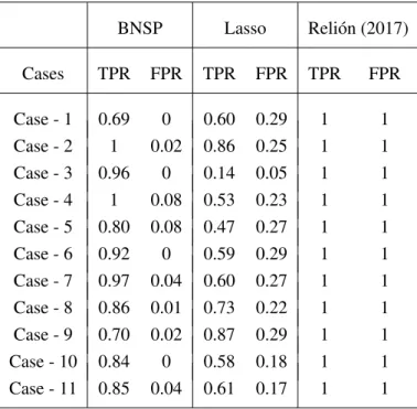
2.7 True Positive Rates (TPR) and False Positive Rates (FPR) for edges for cases in Simulation 1. . . 36

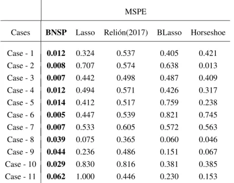
2.9 MSPE under the BNSP vis-a-vis competitors for cases inSimulation 1. Lowest MSPE for any case is made bold. . . 41

2.10 Coverage and length of 95% predictive intervals (PIs) under the BNSP vis-a-vis competitors for cases inSimulation 1. . . 42

(14)

2.11 MSPE, coverage and length of 95% predictive intervals (PIs) under the BNSP vis-a-vis competitors for cases inSimulation 2. Lowest MSPE for any case is made bold.. . . 43

2.12 MSPE, coverage and length of 95% predictive intervals (PIs) under the BNSP vis-a-vis competitors for cases inSimulation 3. Lowest MSPE for any case is made bold.. . . 44

2.13 Performance of Bayesian Network Regression vis-a-vis competitors. Predictive point estimation has been captured through the Mean Squared Prediction Error (MSPE). . . 45

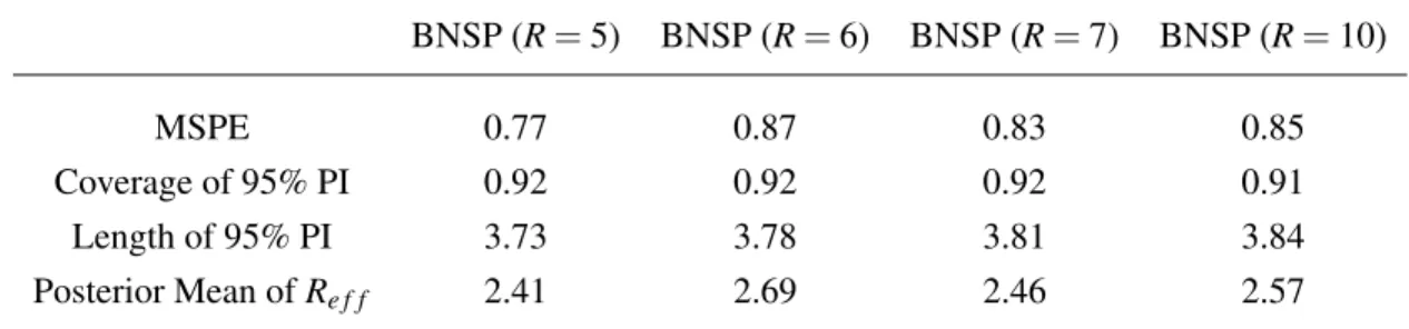
2.14 Model behavior in terms of model performance metrics with changing values ofRfor data corresponding toSimulation 1, Case 9. We report MSE, MSPE, length and coverage of 95% predictive intervals and the posterior mean of ef-fective dimensionalityRe f f.. . . 45

2.15 Computation time of competing methods for different values of sample size (n) and number of nodes (V). For the Bayesian method BNSP, the table records run time (in seconds) per equivalent effective posterior sample for BNSP, to account for the fact that posterior samples are correlated. The last two columns record total run time for frequentist methods. . . 46

(15)

2.16 Predictive performance of competitors in terms of mean squared prediction er-ror (MSPE), coverage and length of 95% predictive intervals, obtained through 10-Fold Cross Validation in the context of real data. Note that since the response has been standardized, an MSPE value greater than or around 1 will denote an inconsequential analysis. . . 52

2.17 Brain regions (ROIs) detected as influential for the composite creativity index by BNSP. . . 54

2.18 Predictive performance of BNSP withR=5,6,7,10 to assess the sensitivity of predictive inference with the choice ofR. . . 54

3.1 Table presents different cases forSimulation 1. The true dimensionRg is the

dimension of vector objectuk,0using which data has been generated. The

max-imum dimensionRis the dimension of vector objectuk using which the model

has been fitted. Node sparsity and residual edge sparsity are described in the text. 69

3.2 Table presents different cases forSimulation 2. The true dimensionRg is the

dimension of vector objectuk,0using which data has been generated. The

max-imum dimensionRis the dimension of vector objectuk using which the model

has been fitted. Node sparsity and residual edge sparsity are described in the text. 69

(16)

3.5 NBL,BH represents the number of edges identified by both BNLC and BNHC.

Similarly,NBLandNBH represent the number of edges identified by BNLC and

BNHC, respectively. Top 10 represents the number of edges common among the top ten edges identified by BNLC and BNHC. Top 20 and Top30 are defined analogously. . . 76

3.6 Performance of BNLC and BNHC vis-a-vis competitors for cases in Simulation 1. Parametric inference in terms of point estimation of edge coefficients has been captured through the Mean Squared Error (MSE). The minimum MSE among competitors for any case is made bold. . . 77

3.7 Performance of BNLC and BNHC vis-a-vis competitors for cases in Simulation 2. Parametric inference in terms of point estimation of edge coefficients has been captured through the Mean Squared Error (MSE). The minimum MSE among competitors for any case is made bold. . . 80

3.8 Mean Squared Error (MSE) of estimating the network coefficient in BNLC and BNHC for different combinations of hyper-parameters. . . 82

3.9 True Positive Rates (TPR) and False Positive Rates (FPR) of identifying influ-ential edges in BNLC and BNHC for different combinations of hyper-parameters. 83

3.10 Nodes identified as influential by both BNLC and BNHC.. . . 88

3.11 Top 100 represents the number of edges common among the top 100 edges identified by BNLC and BNHC. Top 200 and Top 300 are defined analogously. 90

(17)

3.12 Predictive performance of Bayesian Network Classification (BNC) vis-a-vis competitors in terms of Area Under Curve (AUC) of the ROC. AUC has been calculated in each case using 10-fold cross validation. . . 90

3.13 Number of nodes identified as influential for all combinations are presented. The table also presents the number of intersections of influential nodes between different combinations and the original analysis. . . 91

3.14 Number of edges identified as influential for all combinations are presented. The table also presents the number of intersections of influential nodes between different combinations and the original analysis. . . 91

3.15 AUC and posterior mean of effective dimensionality for BNLC and BNHC un-der different choices ofR.. . . 92

4.1 Table presents different cases in the simulation study. The parametersH0, H

refer to the true and fitted number of mixture components in the nonparamet-ric Bayesian network regression model. Different cases also present various combinations of the number of network nodesV and sample sizen. . . 105

4.2 Mean squared error (MSE), coverage and length of 95% credible intervals in estimating the regression function for NBNR and BNSP are provided for all the cases. . . 113

(18)

4.4 Mean squared error (MSE), coverage and length of 95% credible intervals in estimating the regression function for NBNR under different hyper-parameter settings. The last row of the table shows the posterior mean of the number of clusters (M.C. ormean number of clusters) in the five different hyperparameter combinations. . . 116

4.5 Model fitting statistics for NBNR and BNSP for the OCEAN data. . . 123

4.6 Brain regions (ROIs) detected as influential for the two detected clusters of individuals in the OCEAN dataset. . . 123

4.7 Brain regions (ROIs) detected as influential by BNSP in the OCEAN dataset. . 124

4.8 Performance of NBNR under different hyperparameter choices for the OCEAN data. The first column presents different combinations to check sensitivity. the second column presents ARI between optimal clusters obtained from each combination and the optimal clusters obtained by the original analysis of the OCEAN data. . . 128

4.9 Model fitting statistics for NBNR and BNSP for the brain connectome CCI data application. . . 129

(19)

Abstract

On Bayesian Methods in Network Regression by

Sharmistha Guha

There has been a growing interest during recent years in connectomics, which is the study of interconnections or networks within the human brain. This interest has been spurred by the development of new imaging technologies, which allow researchers to peer non-invasively into the human brain and obtain data on connections. Motivated by these datasets, this dissertation develops a novel class of Bayesian regression models which study the relationships between neuro-scientific phenotypes and brain connectome networks of individuals.

First, we introduce a novel approach that develops a regression framework of the brain network (represented in the form of a symmetric matrix) on a continuous phenotypic response. We propose a novel network shrinkage prior on the network predictor coefficient matrix. The proposed framework is able to identify nodes or functional regions in the brain network and interconnections between different regions, significantly related to the phenotypic response. To the best of our knowledge, our framework is the first principled Bayesian framework that enables identification of network nodes and edges significantly related to the response. The performance of the proposed model is evaluated with respect to a wide range of existing com-petitors available in the high dimensional frequentist and Bayesian literature using a variety of simulation studies. The proposed model identifies important brain regions and interconnections

(20)

Next, we extend our model to build network classifiers when a brain connectome net-work along with a binary response is provided for a group of individuals. Here we develop a broader class of global-local network shrinkage priors which includes the novel prior distri-bution specified earlier as a special case. We specifically consider two different global-local network shrinkage priors from this class of priors and investigate them using simulation stud-ies. In particular, we assess their performance in terms of network classification and identifying influential network nodes and edges for the purpose of classification. We also demonstrate su-perior performance of our proposed network classifiers over state-of-the-art high dimensional classification techniques. Another major contribution remains developing theoretical conditions to guarantee asymptotically consistent classification for the proposed framework. In particular, we derive conditions on the number of network nodes, sparsity in the network coefficient ma-trix as a function of the sample size to achieve asymptotically optimal classification. While theoretical results on high dimensional binary regression with ordinary shrinkage priors have emerged recently, developing theory for our network classifier model involves several addi-tional challenges due to the complex nature of the global local shrinkage prior developed here. The framework is used to classify individuals into high and low IQ groups based on their brain connectomes.

Notably, the work discussed in the last two paragraphs tacitly assumes that all nodes and edges have similar impact on a phenotype for every individual. In our next project, we study a brain connectome data where this assumption is violated. In fact, there is a relatively less developed literature in neuroscience that argues for different groups of individuals having shared relationships between brain networks and phenotypes, though this literature lacks a principled

(21)

Bayesian approach that takes into account different relationships of nodes and edges with the response for different groups of individuals and facilitates clustering of individuals. Motivated by this problem and our dataset, we have developed a Bayesian network mixture regression model. Simulation studies and analysis of the brain connectome dataset demonstrate superior performance of the proposed approach over the approach described earlier. Simulation studies are also used to evaluate the performance of the proposed approach by varying the true and fitted number of clusters, size of the network and sample size.

For these projects, computationally efficient Bayesian sampling algorithms are de-veloped to enable computations even for reasonably large networks in presence of moderately large sample size.

(22)

To Shruti, the joy of my life; to my parents Subrata and Shorashi, for their unceasing love and care; and to Rajarshi, my friend, philosopher and guide, without whose

(23)

Chapter 1

Introduction

1.1 Terminology and Network Properties

Interconnections among independent (or otherwise) components of a system can yield valuable information and may be of scientific interest in several scenarios. The intercommunica-tion between these components (or actors) along with the structure formed by them is generally

known as anetworkor agraph. One may find several applications of networks in fields such

as the bio-sciences (eg. genetic interactions, protein networks), epidemiology (transmission of infectious diseases), the social sciences (social relationships and interactions), political science (international relations), finance (interactions between multinational corporations, economic interactions between various economies) and engineering (communication networks, networks across the internet) to name a few.

Network data is challenging to analyze, not only because it requires dimensionality reduction procedures to effectively deal with the large number of pairwise relationships, but

(24)

also because flexible formulations are needed to account for the topological structure of the network. In addition to creating models that can efficiently explain the network structure, it is also of scientific interest to make predictions about missing and/or future relationships between network nodes and edges. An advantage of creating effective statistical models to explain and make predictions regarding networks is that they come with measures of uncertainty around the estimates and predictions.

The simplest form of network is abinary networkin which the edges simply denote

connection or lack of the same amongst any pair of nodes, thus being dichotomous in nature. Examples of this type of network could include ones providing information on whether a pair of actors are friends or not, or whether they are involved in a conflict or not, and so on. A

network might also be one in which the edges areweighted. The weights may denote counts,

e.g., distance or the number of transactions of a specific kind between a pair of nodes. Such a

network is commonly known as avaluedor aweightednetwork.

Networks may also be classified asdirectedorundirected. A directed (or asymmetric)

relationship between a pair of actors would consist of two values, each value representing the stance of one actor towards the other. On the other hand, an undirected (or symmetric) relation-ship would consist only of a single value representing the stance of each pair of members. A simple example of an undirected network would be a brain imaging network where the relation-ship between a pair of regions of interest in the brain is captured by a single value. On the other hand, an example of a directed network could be a social influence network in which there is an influencer whose opinions or actions influence several followers but not the other way round.

(25)

net-work withV nodes, the adjacency matrix is aV×V matrix, with the cell entries being

dichoto-mous or continuous depending on whether the network is binary or weighted, respectively. The matrix would be symmetric or asymmetric depending upon the nature of the relationships between pairs of nodes, i.e. whether they are undirected or directed. Also, if there are no

self-relationships, diagonal elements are not modeled. Notationally,A= ((ak,l))Vk,l=1will be used to

denote theV×V adjacency matrix corresponding to a network, whereak,l corresponds to the

weighted or unweighted relationship between nodes kandl. Again, a network is often

asso-ciated with edge specific covariates. LetX = [xk,l]be a covariate array of predictor variables

xk,l corresponding to dyad(k,l). Sometimes covariates are available corresponding to every

node, referred to as node specific attributes. Mathematically, we denote the attribute vector

corresponding to thekth node byhk.

There are various approaches in the literature in order to visualize and characterize networks, several of them being graph-theoretic in nature. Of course, the most appropriate way to visualize a network in a given context depends on the scientific question at hand. A review

of network properties and measure summaries can be found in [140]; [104] and [103].

There are certain measures which are often used in the literature to summarize a

network. A very important measure in the characterization of a network is thedegree of its

nodes. The degree of a node is the number of edges connected to that node. This is a measure of

the extent of “connectedness” of each of the nodes in a network. Another measure is thevertex

centrality which gauges the relative importance of a node in a network and is usually based

on thegeodesic distanceor shortest distance between two nodes [140]; [86]. The connectivity

(26)

nodes of a network based on their corresponding attributes is known ashomophilyorassortative

mixingand is often encountered in social networks. Acute cases of homophily in which the

network exhibits strongcommunity structure, or in other words, a situation in which subsets of

nodes or actors display cohesive patterns as a result of the underlying relational framework, also constitute an active field of research.

1.2 Statistical models for networks

Some of the pioneering work in the statistical modeling of networks dates back to the late 1950s and early 1960s. Prevailing literature in this field deals mainly with single network observations, with or without accompanying information on nodal attributes. By and large, the relationship between network and nodal attributes has been studied using two separate ap-proaches. One of these approaches focuses on modeling the structure of the network conditional of the nodal attributes. The goal in this case is to understand how social relationships are formed based on attributes of individuals, a process known as “selection”. The other approach consists of models of the nodal attributes and their association conditional on the network structure. These models are employed to understand how relationships affect attributes of the individuals in a network, a process referred to as “influence” or “contagion.” Additional scenarios include the one in which the network and nodal attributes are jointly modeled. Another scenario of in-terest is when a response (continuous, binary or categorical) is regressed on a network, leading to a network regression problem, which is extensively studied in this proposal. We proceed to discuss each scenario in more detail below.

(27)

1.2.1 Models for Selection

Some of the pioneering work in the statistical modeling of networks dates back to the late 1950s and early 1960s. Prevailing literature in this field deals mainly with single network observations, with or without accompanying information on nodal attributes. More specifically, in most of the existing literature, a single network is subjected to an unsupervised analysis using

random graph models [39]; [56], exponential random graph models [49], social space models

[72]; [67], stochastic block models [106], bilinear mixed models [67] or eigenmodels [68]. We

offer brief descriptions on these classes of models below.

Therandom graph model[39]; [56] is one of the foremost network models in the

lit-erature and is constructed in such a way that the edge between any pair of nodes is incorporated into the graph independently and with a fixed probability. In most real-world scenarios, the

distribution of thedegreeof a network turns out to be positively skewed, since only a few nodes

are expected to be very highly connected. This is a drawback for the random graph models since they imply a lighter tailed distribution of the degree. They are also more inclined to be dense, have small diameter and low clustering, which make them unrealistic for practical purposes.

More realistic situations in network data are accommodated by theexponentially

pa-rameterized random graph models(ERGM), also known as thep∗models [49]; [141]. ERGMs

are expressed in exponential form and usually involve some summary statistics of the network. Specifically, the probability mass function for an ERGM is given by

p(A|X,θ) =exp

∑Kk=1θkSk(A,X)

κ(θ)

(28)

rameter vector and κ(θ) is a normalizing constant. Recall that examples of network statistics

include degree, vertex centrality, cohesion and homophily, as described in section1.1. ERGMs,

though having some desirable features, have some shortcomings. They can be computationally challenging and can have the issue of model degeneracy (i.e. putting inordinate importance to

a few network configurations). A detailed treatment of ERGMs can be found in [115] and [96].

A broad class of network models can be included under the umbrella ofsocial space

models. In the realm ofsocial space models, the use ofrandom effectsin the context of probit or

logistic regression to model binary networks has also become popular in recent times. Consider

a probit model (the logistic model is analogous and has been used by [72] and [67] in which the

ak,l’s are conditionally independent with probability of interaction

θk,l ≡p(ak,l=1|β,γk,l,xk,l) =Φ(xTk,lβ+γk,l); k,l=1, ...,V;k<l

whereΦdenotes the cumulative distribution function of a standard normal random variable,β

is an unknown vector of fixed effects andγk,lis an unobserved dyad(k,l)-specific random effect

unrelated to the predictor variable.

If the matrix of random effectsΓ= [γk,l]is jointly exchangeable, there exists a

sym-metric functionα(·,·) such thatγk,l =α(uk,ul) whereuk,k∈ {1, ...,V} [4]. The form of the

function α(·,·) is directly associated with the important structural characteristics of the

net-work. There have been a number of alternatives to select the latent factors which give rise to

different classes of social space models. For example,stochastic block models[106] assume

(29)

distri-bution characterizing the relationship between each pair of nodes. Here the latent effects are

specified asα(uk,ul) =muk,ul, whereuk,ul∈ {1,2,3, ...,R},Ris the number of latent classes,

and also mr,s∈

R

andmr,s=ms,r. Latent distance models [72], on the other hand, assume

thatα(uk,ul) =−|uk−ul|, where| · |denotes the euclidean norm. The underlying assumption

here is that the probability of an edge between two nodes increases as the latent characteristics

of these nodes come closer in terms of their euclidean distance. Bilinear models[67] assume

that the probability of an edge between two nodes is a symmetric multiplicative effect. The

multiplicative interaction for a dyad(k,l)is expressed in terms of abilinear effect, i.e. the inner

product of the unobserved latent vectorsuk andul. Hence, the latent effects are specified as

α(uk,ul) =ukTul, whereuTkul is the bilinear effect. The rationale behind this type of models is

that the probability of an edge between two nodes increases as the angle formed by the

corre-sponding latent positions becomes wider, i.e. nodeskandlwould be prone to having a tie if the

angle between them is acute (uT_kul>0), neutral to a tie if the angle is a right angle (uTkul =0)

and averse to having a tie if the angle between them is obtuse (uT_kul <0). Bilinear models can

generalize distance models, but not latent class models, since the eigenvalues of latent class

models may be negative [68].Eigenmodels[68] are a generalization of the latent class and

la-tent distance models due to the fact that they can be used to represent the same network features but not the other way round. These models are based on the principles of eigen-analysis and render the relationship between two nodes as the inner-product of node-specific latent vectors,

(30)

1.2.2 Models of Contagion

Models of contagion are usually constructed by regressing a nodal attribute on the

attributes of other nodes in the social network (e.g., see [24]; [47]; [124] and references therein),

with common methodological approaches including simultaneous autoregressive (SAR) models

[94] and threshold models [142]. For instance, node specific responses{yk:k∈ {1, ...,V}}are

regressed on the node specific attributes using the simultaneous autoregressive models (SAR) that respect the network structure.

1.2.3 Joint Modeling of Network and Attributes

It is usually a complicated problem to ascertain the direction of a causal relationship between network structure and link or nodal attributes, i.e. whether it pertains to selection or

contagion [33]. Hence, a section of the literature focusses on jointly modeling the co-evolution

of network and nodal attributes through shared latent variables. In recent years, joint models

of network and attributes have been receiving increased attention. [46] have recently proposed

an extension of the bilinear model of [67] in a static setting where the nodal attributes and

la-tent factors used to describetransitivity (the extent to which the relation between two nodes

in a network that are connected by an edge is transitive) in the network are jointly modeled

using a multivariate normal distribution. [36], on the other hand, propose joint modeling of

a binary/categorical response and a network using latent variable tensor factorization of the

joint probability model. [30] have proposed time varying joint models for network and

(31)

the framework to accommodate continuous nodal attributes. [61] propose a Bayesian approach to inference, testing and prediction for co-evolving networks and nodal attributes by accommo-dating both discrete and continuous attributes and considering the more general case of time series data. They use a common set of latent factors to explain network transitivity and covari-ation among attributes and network structure, and provide a fully Bayesian test of associcovari-ation in order to study individual nodal attributes. When the nodal attributes are assumed to fol-low conditional Gaussian distribution, their model can be interpreted as a dynamic version of

the model presented in [46], with a structured and more parsimonious prior on the covariance

matrix between the latent traits and the nodal attributes.

1.2.4 Models for Network Regression

Previous models focus on the analysis of a single network. There are situations in which a network is collected for each observational unit. This is especially pertinent to bio-logical and physiobio-logical problems wherein, for example, each node corresponds to a certain fixed location in the human brain or a particular genetic unit in a gene network. Furthermore, the data might contain a continuous or categorical outcome corresponding to each individual in the sample, possibly associated with the network. Examples of such datasets include brain

connectome applications for multiple individuals which we discuss in detail in Chapters2, 3

and4. The nodes in the network correspond to the brain regions of interest (ROI) shared by all

individuals in the sample and are registered by mapping every brain to a common brain atlas. Additionally, data on a phenotype is available for every individual. For example, the phenotype

(32)

Cre-ativity Index(CCI). Sometimes the outcome can be binary representing whether a subject has

‘high’ or ‘low’ IQ.

In relating the response to the undirected network, a common approach would be to vectorize the network predictor (originally obtained in the form of a symmetric matrix) and treat

it as a collection of a large number of edge weights [114]; [27]. Subsequently, the response

would be regressed on the high dimensional collection of edge weights. This idea can take advantage of the recent developments in high dimensional regression, consisting of both

penal-ized optimization [133] and Bayesian shrinkage [109],[17],[5] perspectives. Additionally, these

models are computationally convenient and are generally accompanied by theoretical guaran-tee. While the predictive performance of these methods turns out to be satisfactory, their in-terpretability is limited to individual edge selection, which is scientifically less interesting than identifying nodes impacting the response. Furthermore, they ignore the network structure, i.e. the relevant wiring mechanism in the brain architecture for brain connectome analysis, which may contain a plethora of scientific information.

While there are existing approaches for network classification, most of them fail to in-corporate the full network information in the process of classification and rather use a few

sum-mary measures from the network, for e.g. see [11] and references therein. [113] have recently

proposed a penalized optimization scheme that not only enables classification of networks, but also identifies important nodes and edges. Although their framework is demonstrated for classi-fication purposes, it can be adapted to facilitate regression settings (as described in Chapter 2). One key shortcoming of this approach is that it is unable to provide any measure of predictive uncertainty. The need for valid measures of uncertainty on parameter (predictive) estimates is

(33)

crucial, especially in settings with low or moderate sample sizes with complex predictor depen-dence, which naturally motivates our Bayesian approach.

There are recent Bayesian approaches which propose joint modeling of response and

predictors, see e.g. [36]. However, these methods are somewhat restrictive for multiple reasons.

First, their approach is heavily dependent on the assumption that the network is binary and does not find easy extension when the network is weighted. Secondly, their modeling perspective focuses on the classification of a population of networks into two groups and does not assume

easy extension to regression settings. In a separate approach, [137] regress a network response

on a scalar predictor, which is a different problem from the one we are interested in.

1.3 Thesis Outline

In Chapter2we develop a novel framework to answer some important questions

aris-ing from datasets of these types. Primarily, in Chapter2, our inferential focus lies in developing

a high-dimensional regression model of a continuous response on the network predictors that employs all edge weights, but aims at identifying influential nodes and edges to yield

scien-tifically meaningful results. To this end, we construct a novel Bayesian network shrinkage

prior that incorporates network information in the coefficients corresponding to the network

predictors through a social space model [72] with latent variables embedded within a Bayesian

shrinkage prior [109], [17], [5]. We index these latent variables by nodes in the network and

incorporate a spike-and-slab variable selection prior to choose the relevant node specific latent variables explaining variation in the response. The proposed framework is simple enough to

(34)

allow computation through a data-augmented Gibbs sampler. We make the practical benefit of the proposed approach in terms of inference and prediction amply clear by comparing it to other existing methods in various simulation studies. Further, we provide detection of influential brain regions and influential interconnections between different regions responsible for creativity of individuals in a principled Bayesian way which was hitherto not present in the literature. The

model provides additional inferences which can be found in Chapter2.

Chapter3focuses on a network classification problem where a binary response along

with a network is available from every subject. The aim lies in developing a classification of subjects, along with identifying network nodes and edges influential for the purpose of classifi-cation. We broadens the formulation of Bayesian network shrinkage prior developed in Chapter

2and propose a new class of Bayesian network global-local shrinkage prior that includes the

network shrinkage prior formulated in Chapter 2 as a special case. Simulation studies show

superior performance of the proposed formulation over the existing network classification mod-els. We employ the framework to analyze a dataset that aims at classifying subjects into a ‘low’ or ‘high’ IQ group based on her/his brain connectome network. One important contribution

of Chapter3remains theoretical study of asymptotic properties of the posterior distribution for

binary network regression model. In particular, we offer theoretical conditions to ensure

asymp-totically optimal classification from the binary network regression model proposed in Chapter3.

The proofs of the theoretical results in Chapter3can be easily adapted to show the consistency

of the posterior distribution for the model proposed in Chapter2.

Chapter 4presents a brain connectome dataset with a phenotype and brain

(35)

net-work regression model proposed in Chapter2 seems inadequate. Indeed, there is a literature in neuroscience arguing differential relationships between brain networks and human creativ-ity for different groups of individuals. In particular, they argue that the relationship may be very different from people with high IQ compared to people with low IQ. To address this issue,

Chapter4proposes a Bayesian network mixture regression model, allowing for different

net-work regression models for different groups of subjects. Finally, Chapter7presents appendices

(36)

Chapter 2

Bayesian Regression with Undirected

Network Predictors with an

Application to Brain Connectome Data

2.1 Introduction

In recent years, network data has become ubiquitous in disciplines as diverse as neuro-science, genetics, finance and economics. Nonetheless, statistical models that involve network data are particularly challenging, not only because they require dimensionality reduction pro-cedures to effectively deal with the large number of pairwise relationships, but also because flexible formulations are needed to account for the topological structure of the network.

(37)

rela-tionship between node-level covariates and the structure of the network. A number of classic models treat the dyadic observations as the response variable, examples include exponential

random graph models [49], social space models [72,67,68] and stochastic block models [106].

The goal of these models is often either to predict unobserved links or to investigatehomophily,

i.e., the process of formation of social ties due to matching individual traits. Alternatively,

mod-els that investigateinfluenceorcontagionattempt to explain the node-specific covariates as a

function of the network structure (e.g., see [24]; [47]; [124] and references therein). Common

methodological approaches in this context include simultaneous autoregressive (SAR) models

[94] and threshold models [142]. However, ascertaining the direction of a causal relationship

between network structure and link or nodal attributes, i.e., whether homophily or contagion

are in play, is difficult (e.g., see [33] and [120] and references therein). Hence, there has been a

growing interest in joint models for the coevolution of the network structure and nodal attributes

[46,36,30,105,61].

In this chapter we investigate Bayesian models for network regression. Unlike the problems discussed above, in network regression we are interested in the relationship between the structure of the network and one or more global attributes of the experimental unit on which the network data is collected. As a motivating example, we consider the problem of predicting the composite creativity index of individuals on the basis of neuroimaging data measuring the connectivity of different brain regions. The goal of these studies is twofold. First, neurosci-entists are interested in identifying regions of the brain that are involved in creative thinking. Secondly, it is important to determine how the strength of connection among these influential regions affects the level of creativity of the individual. To address these challenges we construct

(38)

a novel Bayesian network shrinkage prior that combines ideas from spectral decomposition

methods and spike-and-slab priors to generate a model that takes into account the structure of the predictors. The model produces accurate predictions, allows us to identify both nodes and links that have influence on the response, and yields well-calibrated interval estimates for the model parameters.

A common approach to network regression is to use a few summary measures from

the network in the context of a flexible regression or classification approach (e.g., see [11] and

references therein). Clearly, the success of this approach is highly dependent on selecting the right summaries to include. Furthermore, this kind of approach cannot identify the impact of specific nodes on the response, which is of clear interest in our setting. Alternatively, a number of authors have proceeded to vectorize the network predictor (originally obtained in the form of a symmetric matrix). Subsequently, the continuous response would be regressed on the high

di-mensional collection of edge weights [114,27]. This approach can take advantage of the recent

developments in high dimensional regression, consisting of both penalized optimization [133]

and Bayesian shrinkage [109,17,5]. However, this approach treats the links of the network as

if they were fully exchangeable, ignoring the fact that coefficients that involve common nodes can be expected to be correlated a priori. Ignoring this correlation is known to lead to poor predictive performance and to potentially impact model selection.

Recently, [113] proposed a penalized optimization scheme that not only enables

clas-sification using network predictors, but also identifies important nodes and edges. Although this model seems to perform well for prediction problems, uncertainty quantification is

(39)

Modifications of the bootstrap that produce well-calibrated confidence intervals in the context

of standard Lasso regression have been proposed [22], but it is not clear whether they extend to

the kind of group Lasso penalties discussed in [113]. Recent developments on tensor regression

[147, 62] are also relevant to our work. However, these approaches tend to focus mainly on

prediction and identification of important edges, but are not designed to detect important nodes impacting the response.

The rest of the chapter evolves as follows. Section 3.2 proposes the novel network

shrinkage prior and discusses posterior computation for the proposed model. Empirical

investi-gations with various simulation studies are presented in Section2.3, while Section2.4analyzes

the brain connectome dataset. We provide results onregion of interest (ROI) andedge

selec-tion and find them to be scientifically consistent with previous studies. Finally, Secselec-tion 2.5

concludes the chapter with an eye towards future work.

2.2 Model Formulation

2.2.1 Definitions and Notations

Letyi andAi ∈RV×V represent the observed scalar response and the corresponding

weighted undirected network for thei-th sample,i=1, . . . ,n, respectively. Depending on the

problemyi is continuous or binary. For example, yi ∈R is continuous in Chapters2 and 4,

andyi∈ {0,1}is binary in Chapter3. All graphs share the same labels on their nodes. In all

our applications,Aiencodes the strength of the network connections between different regions

(40)

with the(k,l)-th entry of Ai denoted byai,k,l∈R. We focus on networks that contain no self

relationship, i.e.,ai,k,k≡0, and are undirected (ai,k,l=ai,l,k). The brain connectome application

considered here naturally justifies these assumptions. Although we present our models specific to these settings, it will be evident that the proposed model can be easily extended to directed networks with self-relations. Throughout all chapters, we denote the Frobenius inner product

between twoV×V matrices A andB by hA,BiF =Trace(B0A). Frobenius inner product is

the natural inner product on the space of matrices and is a generalization of the dot product

from vector to matrix spaces. Frobenius norm of a matrixAis defined as||A||F =

p

hA,AiF.

Additionally, for any vectora= (a1, ...,ap)0, define theL1,L2andL∞norms by||a||1=∑l=p 1|al|,

||a||₂=

q

∑_l=p ₁a2l and||a||∞=max

l |al|respectively. || · ||0denotes theL0-norm, i.e. the number

of non-zero entries for vectors. The || · ||1, || · ||2 and|| · ||∞ norms of a matrix are defined

analogously. All vectors and matrices are denoted by lowercase bold letters and uppercase bold letters respectively.

2.2.2 Bayesian Network Regression Model

We propose the high dimensional regression model of the response yi for the i-th

individual on the undirected network predictorAi= ((ai,k,l))Vk,l=1as

yi=µ+hAi,BiF+εi, εi iid

∼N(0,τ2), (2.1)

whereBis the symmetric network coefficient matrix of dimensionV×V whose(k,l)-th element

is given byγk,l/2 andhAi,BiF =Trace(B0Ai)denotes the Frobenius inner product betweenAi

(41)

generalization of the dot product from vector to matrix spaces. Note that, similar to the network

predictor, the network coefficient matrix B is assumed to be symmetric with zero diagonal

entries. The parameterτ2is the variance of the observational error.

Since self relationship is absent and bothAiandBare symmetric,

hAi,BiF = ∑

1≤k<l≤V

ai,k,lγk,l, and (2.1) can be rewritten as

yi=µ+

∑

1≤k<l≤V

ai,k,lγk,l+εi, εi∼N(0,τ2). (2.2)

Equation (2.2) connects the network regression model with the linear regression framework

withai,k,l’s as predictors andγk,l’s as the corresponding coefficients. However, while in ordinary

linear regression the predictor coefficients are indexed by the natural numbers

N

, Model (2.2)

indexes the predictor coefficients by their positions in the matrix B. This is done in order to

keep tabs not only on the edge itself but also on the nodes connecting the edges.

2.2.3 Developing the Network Shrinkage Prior

Vector Shrinkage Prior

High dimensional regression with vector predictors has recently been of interest in Bayesian statistics. Continuous shrinkage priors, which strongly shrink coefficients ing to unimportant variables to zero while minimizing the shrinkage of coefficients correspond-ing to influential variables, have become particularly popular. Many of these priors can be

ex-pressed as a scale mixture of normal distributions, commonly referred to asglobal-local scale

(42)

precisely, in the context of model (2.2), a global-local scale mixture prior would take the form

γk,l∼N(0,sk,lτ2), sk,l ∼g1, τ2∼g2, 1≤k<l≤V.

Note thats1,2, . . . ,sV−1,V are local scale parameters controlling the shrinkage of the coefficients,

whileτ2is the global scale parameter. Different choices ofg1andg2lead to different classes of

Bayesian shrinkage priors. For example, the Bayesian Lasso [109] prior takesg1as exponential

and g2 as the Jeffreys prior, the Horseshoe prior [17] takes both g1 and g2 as half-Cauchy

distributions, and the Generalized Double Pareto Shrinkage prior [5] takesg₁ as exponential

andg2as the Gamma distribution.

The direct application of this global-local prior in the context of (2.2) is unappealing.

In practice, we expect the matrix of coefficientsB(which itself can be regarded as describing a

weighted network) to exhibit transitivity effects, i.e., we expect that if the interactions between

regionsiand jand between regionsiandkboth influence the response, the interaction between

regions j and k will also be influential [93]. Ordinary global-local shrinkage priors do not

necessarily conform to such an important restriction.

Network Shrinkage Prior

We propose a shrinkage prior on the coefficientsγk,l and refer to it as theBayesian

Network Shrinkage prior(BNSP). The prior borrows ideas from low-order spectral

representa-tions of matrices, and aims to capture transitivity effects in the matrix of regression coefficients. Letu1, . . . ,uV ∈RR be a collection ofR-dimensional latent variables, one for each node, such

(43)

can be represented as a location and scale mixture of normals. More precisely,

γk,l|sk,l,uk,ul,τ2∼N(u0kΛul,τ2sk,l), sk,l∼Exp(θ/2), θ∼Gamma(ζ,ι), (2.3)

wheresk,lis the scale parameter corresponding to eachγk,l, andΛ=diag(λ1, . . . ,λR)is anR×R

diagonal matrix withλr∈ {0,1}. Conditional on the latent variables uk, ul andΛ, ifsk,l =0

then (4.5) implies a reduced rank-decompositionΓ=2B=U0ΛU, whereU is anR×V matrix

whosek-th column corresponds touk andΓ= ((γk,l))Vk,l=1. Drawing intuition from [67], we

can interpret the latent vectorsu1, . . . ,uV as the positions of the nodes in a latent “social” space,

with the strength of the edge effect being controlled by the angular distance between the vectors.

In this interpretation, ∑Rr=1λr=Re f f ≤R, represents theeffective dimensionalityof the latent

space. The effect of the interaction between thek-th andl-th nodes has a positive, negative or

neutral impact on the response depending on whether the node specific latent variablesuk and

ul are in the same direction, opposite direction or orthogonal to each other respectively. In other

words, whether the angle betweenukandul is acute, obtuse or right, i.e.,u0kΛul >0,u0kΛul<0

oru0_kΛul=0 respectively. This kind of bilinear structure is commonly used to model social and

biological networks because of its ability to capture the kind of transitive effects we discussed

before [67,66].

In order to learn which components ofuk are informative for (4.5), we assign a

hier-archical prior

λr∼Ber(πr), πr∼Beta(1,rη), η>1.

The choice of hyper-parameters of the beta distribution is crucial. In particular, note

(44)

The first property provides (weak) identifiability of the different latent dimensions, while the

second ensures that limR→∞var(uk)<∞as long as the prior for the uk’s has a finite second

moment. In fact, we can think of our model as a level-Rtruncation of an infinite dimensional

model, similar in spirit to the stick-breaking construction of the Indian Buffet process [132].

Therefore, as long asRis chosen to be “large enough”, the inferences will be roughly invariant

to this choice. In our illustrations, we perform sensitivity analyses to determine an optimal value

ofRthat maintains computational efficiency, and at the same time ensures the robustness of the

results.

In order to determine which nodes are most influential in explaining the response, we

assign aspike-and-slabmixture prior [76] to the latent factoruk,

uk∼        N(0,M), ifξk=1, δ0, ifξk=0, ξk∼Ber(∆), (2.4)

where δ0 is the Dirac-delta function at 0 and M is a covariance matrix of order R×R. The

parameter∆corresponds to the probability of the nonzero mixture component. Note that if the

k-th node of the network predictor is not influential in predicting the response then, a-posteriori,

ξk should provide high probability to 0. Thus, based on the posterior probability ofξk, it will

be possible to identify unimportant nodes, which we loosely refer to as “uninfluential nodes”, in the network regression.

The rest of the hierarchy is accomplished by assigning prior distributions on∆andM

as follows:

(45)

whereIW(ν,I)denotes an Inverse-Wishart distribution with identity scale matrixIand degrees

of freedom ν. Finally, we choose a non-informative prior on (µ,τ2) such that p(µ,τ2)∝ _τ12.

Appendix A shows the propriety of the posterior distribution under this prior.

The previous discussion assumes that we have conditioned on the latent positions u1, . . . ,uV and the local scale parameters(sk,l). Now that we have described the full hierarchical

structure of the model, it is instructive to briefly discuss the structure of the marginal prior distri-bution obtained after integrating these latent variables. In this regard, note first that integrating

over thesk,l’s alone leads to double exponential priors that are reminiscent of the Lasso. On

the other hand, while no closed form expression exists for the marginal prior after integrating u₁, . . . ,uV, it is easy to see that, marginally, the edge coefficients have mean zero and are not

independent. Hence, from this point of view, the latent positions u1, . . . ,uV simply provide a

mechanism to sparsely model the prior dependence among coefficients.

2.2.4 Posterior Computation

Although summaries of the posterior distribution cannot be computed in closed form, full conditional distributions for all the parameters are available and correspond, in most cases, to standard families. Thus, posterior computation can proceed through a Markov chain Monte

Carlo algorithm. We note, however, that a naive implementation of such algorithm to updateΓ

would have complexityO(q3), whereq=V(V−1)/2. The resulting algorithm would therefore

be computationally too expensive for situations such as our real data application, whereV=68

andq=2278. To address this issue, we follow [8], who propose the use of the Woodbury matrix

(46)

with which this chapter is concernedn is typically much smaller than q, this approach leads

to substantial computational savings that make real-life applications feasible. Details of all the Markov chain Monte Carlo algorithm are presented in Appendix B.

While inferences on the latent positions u₁, . . . ,uV is not our main focus, being able

to visualize these positions can be helpful in terms of interpreting the model results. However,

note that vectors u1, . . . ,uV are not identifiable because the model is invariant to rotations of

the latent space. Hence, before we can use the posterior samples generated by our algorithm to conduct inferences on these latent positions we must first rotate them to a common orientation.

This is done using a “Procrustean” transformation [125,72,67]. For each posterior sampleU(`)

we find the rotation ˜U(`)that has the smallest sum of squared deviations from an arbitrary fixed

reference matrixU0. This rotation is given by ˜U(`)=U0 U(`)

0n

U(`)U0₀U0 U(`) 0o−1/2

U(`).

In our analysis, we use the first iterate after burn-in,U(1), as the reference matrixU0.

In order to identify whether the k-th node is important in terms of predicting the

response, we rely on the post burn-in L samples ξ(_k1), . . . .,ξ(L)_k of ξk. Node k is said to be

influential if 1_L∑L_l=₁ξ(l)_k >0.5. To identify influential edges we utilize a modification of the

algorithm proposed in [92] that allows us to estimate the false discovery rate of the procedure

as a function of the number of discoveries. Details are provided in Appendix C. Finally, an

estimate ofP(Re f f =r|Data)is given by _L1∑L_l=₁I(∑Rm=1λ

(l)

m =r), whereI(A)for an eventA

is 1 if the eventAhappens and 0 otherwise, and λ(m1), . . . ,λ(L)m are theL post burn-in MCMC

(47)

2.3 Simulation Studies

This section comprehensively contrasts both the inferential and predictive perfor-mances of our proposed approach with a number of competitors in various simulation settings. As competitors, we consider both penalized likelihood methods as well as Bayesian shrinkage priors for high-dimensional regression.

Our first set of competitors use generic variable selection and shrinkage methods that treat edges between nodes as “bags of predictors” and rely on high dimensional regression,

thereby ignoring the relational nature of the predictor. More specifically, we use Lasso [133],

which is a popular penalized optimization scheme, and the Bayesian Lasso [109] and Horseshoe

priors [17], which are popular Bayesian shrinkage regression methods. The Horseshoe in

par-ticular is considered to be a state-of-the-art Bayesian shrinkage prior and is known to perform

well, both in sparse and not-so-sparse regression settings. We use theglmnetpackage inR[50]

to implement Lasso regression, and themonomvnpackage inR[59] to implement the Bayesian

Lasso (BLasso for short) and the Horseshoe (BHS for short).

A thorough comparison with these methods will indicate the relative advantage of exploiting the structure of the network predictor.

Additionally, we compare our method to a frequentist approach that develops network

regression in the presence of a network predictor and scalar response [113]. To be precise, we

(48)

coefficient matrixBby solving ˆ B=arg min B∈R,B=B0,diag(B)=0 ( 1 n n

∑

i=1 (yi−µ− hAi,BiF)2+ ϕ 2||B|| 2 F+ς V

∑

k=1 ||B_(k)||2+ρ||B||1 ! ) , (2.5) where||B||F = p

hB,BiF denotes the Frobenius norm,||B||1 is the sum of the absolute values

of all the elements of matrixB,|| · ||2 is thel2 norm of a vector,B(k) is thek-th row ofBand

ϕ,ρ,ςare tuning parameters. The best possible choice of the tuning parameter triplet(ϕ,ρ,ς)

is made using cross validation over a grid of possible values. [113] argue that the penalty in

(2.5) incorporates the network information of the predictor, thereby yielding superior inference

to any ordinary penalized optimization scheme. Hence comparison with (2.5) will highlight

the advantages of a carefully structured Bayesian network shrinkage prior over the penalized optimization scheme incorporating network information. In the absence of open source code,

we implemented the algorithm in [113] ourselves. All Bayesian competitors are allowed to draw

50,000 MCMC samples, out of which the first 30,000 are discarded as burn-ins. All posterior

inference is carried out based on the rest 20,000 MCMC samples after suitably thinning the

post burn-in chain. Convergence is assessed by comparing different simulated sequences of

representative parameters started at different initial values [52].

2.3.1 Predictor and Response Data Generation

In all simulation studies, the responseyiis generated according to the network

regres-sion model

(49)

withτ2₀ as the true noise variance. In all of our simulations, we useV =20 nodes andn=70 samples.

Simulation 1

In this group of simulations, the (k,l)-th entry of B₀ is given by w

0

kwl

2 , where the

vectorsw1, . . . ,wV, each of dimensionRgen, are generated from a mixture

wk∼πwNRgen(wmean,w 2

sd) + (1−πw)δ0, k∈ {1, . . . ,V}, (2.7)

whereδ0is the Dirac-delta function andπwis the probability of anywkbeing nonzero.(1−πw)

is the probability of a node not being influential, it is referred to as thenode sparsity parameter.

This data generation mechanism is quite similar (although not identical) to our hierarchical prior. Hence, the goal of this first simulation is to evaluate the ability of the model to recover the true data-generation mechanism and, in particular, its ability to identify the true dimension of the latent space, as well as the sensitivity of the results to the choice of the maximum latent

dimensionR.

For a comprehensive picture ofSimulation 1, we consider 11 different cases as

sum-marized in Table3.1. In each of these cases, the network predictor coefficient and the response

are generated by changing the sparsityπw and the true dimensionRgen of the latent variables

wk’s. The table also presents the maximum dimensionRused to fit the model of the latent

vari-ablesuk for the network regression model (2.2). Note that we include various cases of model

mis-specification in whichR>Rgen. For all simulations,wmean andw2_sd are set as 0.5×1Rgen

andIRgen×Rgen, respectively, and the variance τ

2

(50)

network predictorAi for thei-th sample are simulated from a standard normal distribution. In

Cases 10 and 11 the network predictorAifor thei-th sample follows a stochastic blockmodel.

In Case 10, we assume that each brain network has 3 local clusters with high within-cluster and

low between-cluster connectivity. More specifically, the matricesAi’s consist of 3 symmetric

block diagonal matrices of dimensions 6×6, 7×7 and 7×7 respectively. Elements in these

matrices have been drawn fromN(j,j2) where j∈ {1,2,3}, for the j-th block diagonal. The

off-diagonal blocks are highly sparse with very few randomly chosen non-sparse elements

de-noting connections between nodes in different clusters randomly chosen fromN(0,1). In Case

11, the adjacency matricesAi’s also consists of 3 block diagonal matrices, in this case of

dimen-sions 5×5, 8×8 and 7×7. As before, the elements in these matrices have been drawn from

N(j,j2)where j∈ {1,2,3}, for the j-th block diagonal. However, in this case the elements in

the off-diagonal matrices have been drawn fromN(4,1),N(5,1)andN(6,1).

Simulation 2

In this case, the matrix of coefficientsB0 is constructed by first generatingV binary

indicatorsξ0₁, . . . ,ξ0_V independently from aBer(π2,w), one for each node in the network. If both

ξ0_k=1 andξ0_l =1, the edge coefficient connecting thek-th and thel-th nodes (k<l) is simulated

fromN(0.8,1). Otherwise, we set the(k,l)-th edge coefficient to be 0. Similar toSimulation

1, we refer to 1−π2,was thenode sparsity parameter. While this simulation scenario has some

similarities to our proposed model, the mean effect for active nodes is constant. Therefore, the goal of this simulation is to evaluate the performance of the model in situations where there are

(51)

is simulated by drawing ai,k,l independently from aN(0,1) distribution for k<l and setting

ai,k,l =ai,l,k andai,k,k =0 for allk,l∈ {1, . . . ,V}. Finally, the variance τ2₀ is fixed at 1 as in

Simulation 1. Table2.2presents the two cases we consider forSimulation 2, which are obtained

by varying the node sparsity parameter.

Simulation 3

In this case, we drawV indicator variablesξ0₁, . . . ,ξ_V0 from aBer(π2,w)corresponding

to theV nodes of the network. If bothξ0_k=1 andξ0_l =1, then the edge coefficient connecting

thek-th and thel-th nodes (k<l) is simulated from a mixture distribution given by

π3,w∼NRgen(0.8,1) + (1−π3,w)δ0, k,l∈ {1, . . . ,V}. (2.8)

Otherwise, if ξ0_k =0 for any k, we set(k,l)-th edge coefficient to be 0 for alll. Contrary to

Simulation 2,Simulation 3allows the possibility of an edge between thek-th and thel-th nodes

having no impact on the response even when bothξ0_k andξ0_l are nonzero. In the context of

Simulation 3,(1−π2,w)and(1−π3,w)are referred to as thenode sparsityand theedge sparsity

parameters, respectively. Hence, the goal of this simulation is to evaluate the impact of edge sparsity and its interaction with node sparsity on model performance. Network predictors are

randomly generated using the same mechanism as inSimulation 2 and the true varianceτ2₀ is

again fixed at 1 for all cases. Table2.3presents the four cases we consider in this evaluation,