Does algorithmic trading improve liquidity?

Center for Financial Studies

Goethe-Universität Frankfurt „ House of Finance

Grüneburgplatz 1 60323 Frankfurt Deutschland

No. 2008/41

Does Algorithmic Trading Improve Liquidity?

Terrence Hendershott, Charles M. Jones,

and Albert J. Menkveld

Telefon: +49 (0)69 798-30050 Fax: +49 (0)69 798-30077

Center for Financial Studies

Center for Financial Studies

The

_{Center for Financial Studies}

is a nonprofit research organization, supported by an

association of more than 120 banks, insurance companies, industrial corporations and

public institutions. Established in 1968 and closely affiliated with the University of

Frankfurt, it provides a strong link between the financial community and academia.

The CFS Working Paper Series presents the result of scientific research on selected

topics in the field of money, banking and finance. The authors were either participants

in the Center´s Research Fellow Program or members of one of the Center´s Research

Projects.

If you would like to know more about the

_{Center for Financial Studies}

, please let us

know of your interest.

Prof. Dr. Jan Pieter Krahnen

Prof. Volker Wieland, Ph.D.

* We thank Bruno Biais, Alex Boulatov, Thierry Foucault, Maureen O’Hara, S´ebastien Pouget, the Nasdaq Economic Advisory Board, and seminar participants at the University of Amsterdam, Babson College, Bank of Canada, HEC Paris, IDEI Toulouse, University of Miami, the 2007 MTS Conference, NYSE, University of Utah, and Yale University. We thank the NYSE for providing system order data. Hendershott gratefully acknowledges support from the National Science Foundation; Menkveld gratefully acknowledges the college van Bestuur of VU University Amsterdam for a VU talent grant.

1 Haas School of Business, University of California, Berkeley; e-mail: [email protected]; tel: 510 643-0619

2 Graduate School of Business,Columbia University, 3022 Broadway, Uris Hall 801 New York, NY 10027; e-mail: [email protected]; tel: 212-854-4109

CFS Working Paper No. 2008/41

Does Algorithmic Trading Improve Liquidity?*

Terrence Hendershott

, Charles M. Jones

,

and Albert J. Menkveld

April 26, 2008

Abstract:

Algorithmic trading has sharply increased over the past decade. Equity market liquidity has

improved as well. Are the two trends related? For a recent five-year panel of New York Stock

Exchange (NYSE) stocks, we use a normalized measure of electronic message traffic (order

submissions, cancellations, and executions) as a proxy for algorithmic trading, and we trace

the associations between liquidity and message traffic. Based on within-stock variation, we

find that algorithmic trading and liquidity are positively related. To sort out causality, we use

the start of autoquoting on the NYSE as an exogenous instrument for algorithmic trading.

Previously, specialists were responsible for manually disseminating the inside quote. As

stocks were phased in gradually during early 2003, the manual quote was replaced by a new

automated quote whenever there was a change to the NYSE limit order book. This market

structure change provides quicker feedback to traders and algorithms and results in more

message traffic. For large-cap stocks in particular, quoted and effective spreads narrow under

autoquote and adverse selection declines, indicating that algorithmic trading does causally

improve liquidity.

JEL Classification:

G10

Technological change has revolutionized the way financial assets are traded. Back office improve-ments can support vastly increased trading volume. Retail investors place orders via computer rather than speaking to a broker on the phone. Trading floors have largely been replaced by electronic trading platforms (Jain (2005)).

The nature of order execution has changed dramatically as well, as many market partici-pants now employ algorithmic trading (AT), commonly defined as the use of computer algorithms to manage the trading process. From a starting point near zero about ten years ago, AT is now thought to be responsible for 1₃ of trading volume in the U.S and is expected to account for perhaps

half of trading volume by 2010.1 The intense activity generated by algorithms threatens to

over-whelm exchanges and market data providers,2forcing significant upgrades to their infrastructures.

Before algorithmic trading took hold, a pension fund manager who wanted to buy 30,000 shares of IBM might hire a broker-dealer to search for a counterparty to execute the entire quantity at once in a block trade. Alternatively, that institutional investor might have hired a New York Stock Exchange (NYSE) floor broker to go stand at the IBM post and quietly “work” the order, us-ing his judgment and discretion to buy a little bit here and there over the course of the tradus-ing day to keep from driving the IBM share price up too far. As trading became more electronic, it became easier and cheaper to replicate that floor trader with a computer program doing algorithmic trading (see Hendershott and Moulton (2007) for evidence on the decline in NYSE floor broker activity). Now virtually every large broker-dealer offers a suite of algorithms to its institutional customers to help them execute orders in a single stock, in pairs of stocks, or in baskets of stocks. Algorithms typically determine the timing, price, and quantity of orders, dynamically monitoring market con-ditions across different securities and trading venues, reducing market impact by optimally (and sometimes randomly) breaking large orders into smaller pieces, and closely tracking benchmarks such as the volume-weighted average price (VWAP) over the execution interval. As they pursue a desired position, these algorithms often use a mix of active and passive strategies, employing both limit orders and marketable orders. Thus, at times they function as liquidity demanders, and at times these algorithms supply liquidity.

Many observers think of algorithms from the standpoint of this institutional buy-side

investor.3 But there are other important users of algorithms. Some hedge funds and broker-dealers

supply liquidity using algorithms, competing with designated market-makers and other liquidity suppliers. For assets that trade on multiple venues, liquidity demanders often use smart order routers to determine where to send a marketable order. All of these are also forms of algorithmic trading.4

1_{See “Ahead of the Tape-Algorithmic Trading,”Economist, June 23, 2007.} 2_{See “Dodgy Tickers-Stock Exchanges,”Economist, March 10, 2007.} 3_{See, for example, Domowitz and Yegerman (2005).}

4_{Algorithms can also be used to formulate trading decisions and strategies as well as implement them. There are} clearly feedback effects between the portfolio strategy side and the execution side. For example, algorithmic execution could be the difference in making a trading-intensive algorithmic portfolio strategy feasible. Our data reflect counts

As AT has grown rapidly over the past ten years or so, liquidity in world equity markets has also dramatically improved. Based on these two coincident trends, it is tempting to conclude that algorithmic trading is at least partially responsible. But it is not at all obvious_{a priori} that AT and liquidity should be positively related. If algorithms are cheaper and/or better at supplying liquidity, then AT may result in more competition in liquidity provision, thereby lowering the cost of immediacy. However, the effects could go the other way if algorithms are used mainly to demand liquidity. Limit order submitters grant a trading option to others, and if algorithms make liquidity demanders better able to identify and pick off an in-the-money trading option, then the cost of providing the trading option increases, and spreads must widen to compensate. In fact, AT could actually lead to an unproductive arms race, where liquidity suppliers and liquidity demanders both invest in better algorithms to try to take advantage of the other side, with measured liquidity the unintended victim.

In this paper, we attempt to gauge empirically the relationship between algorithmic trading and liquidity. We use a normalized measure of NYSE electronic message traffic as a proxy for algorithmic trading. This message traffic includes electronic order submissions, cancellations, and trade reports. Because we normalize by trading volume, variation in our AT measure is for the most part driven by variation in limit order submissions and cancellations. This means that our measure is mainly picking up variation in algorithmic liquidity supply. This liquidity supply is likely coming both from proprietary traders making markets algorithmically and from buy-side institutions that are submitting limit orders as part of “slice and dice” algorithms.

AT’s effect on liquidity is assessed using two empirical approaches. First, panel regressions are used to establish that time-series increases in algorithmic trading are associated with more liquid markets. While AT and liquidity move in the same direction during our sample period, it is certainly possible that the relationship is not causal. Thus, the panel regressions are mostly a warmup for the main part of the paper, where we study an important exogenous event that increases the amount of algorithmic trading in some stocks but not others. To establish causality, we use the start of autoquoting on the NYSE as an exogenous instrument for algorithmic trading. Previously, specialists were responsible for manually disseminating the inside quote. This was replaced in early 2003 by a new automated quote whenever there was a change to the NYSE limit order book. This market structure change provides quicker feedback to traders and algorithms and results in more electronic message traffic. The change was also phased in for different stocks at different times, and we take advantage of this non-synchronicity to cleanly identify the effects.

We find that algorithmic trading does in fact improve liquidity for large-cap stocks. Quoted and effective spreads narrow under autoquote. The narrower spreads are a result of a sharp decline in adverse selection, or equivalently a decrease in the amount of price discovery associated with trades. There are no significant effects for smaller-cap stocks, but our instrument is weaker there,

so the problem may be a lack of statistical power.

Surprisingly, we find that algorithmic trading increases realized spreads and other mea-sures of liquidity supplier revenues. This is surprising because we initially expected that if AT improved liquidity, the mechanism would be competition between liquidity providers. However, the evidence clearly indicates that liquidity suppliers are capturing some of the surplus for them-selves. To help make sense of this counter-intuitive result, we introduce the generalized Roll model developed in Hasbrouck (2007), modified to allow algorithmic liquidity supply. The model matches up with all our empirical findings. In particular, it shows that liquidity supplier revenues depend on the degree of competition between the marginal liquidity suppliers. To put it starkly, in a world without algorithms, liquidity supplier revenues depend on the degree of competition between liquid-ity supplier humans. In a world with algorithms, liquidliquid-ity supplier revenues depend on the degree of competition between algorithms. Our results suggest that, at least immediately following the start of autoquote, there could have been less competition between the best algorithms, perhaps because new algorithms require considerable investment and time-to-build.

The paper proceeds as follows. Section 1 discusses related literature. Section 2 describes our data and analyzes algorithmic trading and its impact from 2001 through 2005. Section 3 exam-ines algorithmic trading and liquidity surrounding the NYSE’s staggered introduction of autoquote in 2003. Section 4 discusses and interprets the results, and Section 5 concludes.

1

Related literature

There are very few academic papers that address algorithmic trading directly, and none that tackle the broader effects of algorithmic trading on overall market quality. For example, Engle, Russell, and Ferstenberg (2007) use execution data from Morgan Stanley algorithms to study the tradeoffs between algorithm aggressiveness and the mean and dispersion of execution cost. Domowitz and Yegerman (2005) study execution costs of ITG buy-side clients, comparing results from different algorithm providers.

However, there are several strands of academic literature that touch related topics. Most models take the traditional view that one set of traders provides liquidity via quotes or limit orders and another set of traders initiates a trade to take that liquidity – for either informational or liquidity/hedging reasons. Many assume that liquidity suppliers are perfectly competitive, e.g., Glosten (1994). Glosten (1989) models a monopolistic liquidity supplier, while Biais, Martimort, and Rochet (2000) allow for an arbitrary number of symmetric competing liquidity suppliers and find that liquidity suppliers’ rents decline as the number increases. Our initial expectation is that AT facilitate the entry of additional liquidity suppliers, and reduce their overall rents.

The development and adoption of AT also involves strategic considerations. While algo-rithms have low marginal costs, there may be substantial development costs, and it may be costly to optimize the algorithms’ parameters for each security. The need to recover these costs should lead to the adoption of algorithmic trading at times and in securities where the returns to adoption are highest (see Reinganum (1989) for a review of innovation and technology adoption).

As discussed briefly in the introduction, liquidity supply involves posting firm commit-ments to trade. These standing orders provide free trading options to other traders. Using stan-dard option pricing techniques, Copeland and Galai (1983) value the cost of the option granted by liquidity suppliers. The arrival of public information renders existing orders stale and can move the trading option into the money. Foucault, Ro¨ell, and Sandas (2003) study the equilibrium level of effort that liquidity suppliers should expend in monitoring the market to avoid this risk. Black (1995) proposes to minimize picking-off risk with a new limit order type that is indexed to the over-all market. Algorithms enable this kind of monitoring and adjustment of limit orders in response to public information. In fact, in recent work, Rosu (2006) develops a model that implicitly recog-nizes these technological advances and simply assumes limit orders can be constantly adjusted. In general, if AT reduces the cost of the free trading option implicit in limit orders, then measures of adverse selection should decrease with AT. If some users of AT are better at avoiding being picked off, they can impose adverse selection costs on other liquidity suppliers (similar to the mechanism in Rock (1990)) and even drive other liquidity suppliers out.

AT may also be used by traders who are trying to passively accumulate or liquidate a large position. There are a few papers that derive optimal dynamic execution strategies for such traders. For example, Bertsimas and Lo (1998) find that, in the presence of temporary price impacts and conditional on completing the entire transaction by a fixed date, orders are optimally broken into pieces so as to minimize cost. Almgren and Chriss (2000) extend this by considering the risk that arises from breaking up orders and slowly executing them. Obizhaeva and Wang (2005) optimize assuming that liquidity does not replenish immediately after it is taken but only gradually over time. Many brokers build models with such considerations into their AT products that they sell to their clients. On the empirical side, Keim and Madhavan (1995) provide evidence that large orders are broken up, and Chan and Lakonishok (1995) study institutional orders that are worked over multiple days.

For each component of the larger transaction, a trader (or algorithm) must choose the type and aggressiveness of the order. Cohen et al. (1981) and Harris (1998) focus on the simplest static choice: market order versus limit order. If a trader chooses a non-marketable limit order, the aggressiveness of the order is determined by its limit price (Griffiths et al. (2000) and Ranaldo (2004)). Lo, MacKinlay, and Zhang (2002) find that execution times are very sensitive to the choice of limit price. If limit orders do not execute, traders can cancel them and resubmit them with more aggressive prices. A short time between submission and cancellation suggests the presence of AT,

and in fact Hasbrouck and Saar (2007) find that a large number of limit orders are cancelled within two seconds on the Inet trading platform (which is now Nasdaq’s trading mechanism).

2

Data and full sample analysis

To study the relationship between algorithmic trading and liquidity, we start with a monthly panel of NYSE common stocks. We limit ourselves to the post-decimalization regime because the change to a one penny minimum tick was a structural break that substantially altered the entire trading landscape, including liquidity metrics and order submission strategies. The sample extends for almost five years, beginning in February 2001 and ending in December 2005. We start with a sample of all NYSE common stocks that can be matched across the NYSE’s Trade and Quotes (TAQ) and the CRSP databases and retain the stocks that are present throughout the whole sample period (in order to maintain a balanced panel). Stocks with an average share price of less than $5 are removed from the sample, as are stocks with an average share price of more than $1,000. The resulting sample comprises 943 common stocks.

Stocks are sorted into quintiles based on market capitalization. Quintile 1 refers to large-cap stocks and quintile 5 corresponds to small-large-cap stocks. All variables used in the analysis are 99.9% winsorized (that is, values smaller than the 0.05% quantile are set equal to that quantile, and values larger than the 99.95% quantile are set equal to that quantile).

2.1

Proxies for algorithmic trading

We cannot directly observe whether a particular order is generated by a computer algorithm. For cost and speed reasons, most algorithms do not rely on human intermediaries but instead generate orders that are sent electronically to a trading venue. Thus, the rate of electronic message traffic can be used as a proxy for the amount of algorithmic trading taking place. This proxy is commonly used by market participants, including consultants Aite Group and Tabb Group, as well as exchanges and other market venues.5

For example, in discussing market venue capacity limits following an episode of heavy

trading volume in February 2007, a_{Securities Industry News}report quotes Nasdaq SVP of Nasdaq

transaction services Brian Hyndman, who noted that exchanges have dealt with massive increases in message traffic over the past five to six years, coinciding with algorithmic growth.

“It used to be one-to-one,” Hyndman said. “Then you’d see a customer send ten orders

5_{See, for example, Jonathan Keehner, “Massive surge in quotes, electronic messages may paralyse US market,”}

that would result in only one execution. That’s because the black box would cancel a lot of the orders. We’ve seen that rise from 20- to 30- to 50-to-one. The amount of orders in the marketplace increased exponentially.”6

In the case of the NYSE, electronic message traffic includes order submissions, cancella-tions, and trade reports that are handled by the NYSE’s SuperDOT system and captured in the NYSE’s System Order Data (SOD) database. The electronic message traffic measure for the NYSE excludes all specialist quoting, as well as all orders that are sent manually to the floor and are handled by a floor broker.

[insert Figure 1]

As suggested by the quote above, an important issue is whether and how to normalize the message traffic numbers. The top half of Figure 1 shows the evolution of message traffic over time. We focus on the largest-cap quintile of stocks, as these constitute the vast bulk of stock market capitalization and trading activity. Immediately after decimalization at the start of 2001, the average large-cap stock sees about 35 messages per minute during the trading day. There are a few bumps along the way, but by the end of 2005, there are an average of about 250 messages per minute (more than 4 messages per second!) for these same large-cap stocks. We could, of course, simply use the raw message traffic numbers, but there has been a marked increase in trading volume over the same interval, and without normalization a raw message traffic measure may just be capturing the increase in trading rather than the change in the nature of trading. Therefore, we normalize by calculating for each stock each month the number of electronic messages per $1,000 of trading volume. This normalized measure still rises rapidly over the five-year sample, while measures of market liquidity such as proportional spreads have declined sharply but appear to asymptote near the end of the sample (see, for example, the average quoted spreads in the top half of Figure 2), which occurs as more and more stocks are quoted with the minimum spread of $0.01. Since we are essentially regressing spreads on algorithmic trading measures, we want both measures to have this same general shape over time. Thus, our preferred measure is just the negative reciprocal of the messages per dollar traded. Specifically,algo trad_it is calculated as the negative of trading volume (in thousands of dollars) divided by the number of electronic messages. However, our results are virtually the same when we normalize by the number of trades or use raw message traffic numbers. The results are also the same when we use the number of cancellations rather than the number of messages to construct the algorithmic trading measure.

The time-series evolution of algo trad_it is displayed in the bottom half of Figure 1. For the largest-cap quintile, there is about $7,000 of trading volume per electronic message at the

6_{See Shane Kite, “Reacting to market break, NYSE and Nasdaq act on capacity,”Securities Industry News, March} 12, 2007.

beginning of the sample in 2001, decreasing dramatically to about $1,100 of trading volume per electronic message by the end of 2005. Over time, smaller-cap stocks display similar time-series patterns. Cross-sectionally, there is a positive monotonic relationship between market cap and trading volume per message. In general, we focus more on time-series behavior rather than the cross-sectional patterns.

It is worth noting that our algorithmic trading proxies may also capture changes in trading strategies. For example, messages andalgo trad_itwill increase if the same market participants use algorithms but modify their trading or execution strategies so that those algorithms submit and cancel orders more often. Similarly, the measure will increase if existing algorithms are modified to “slice and dice” large orders into smaller pieces. This is useful, as we want to capture increases in the intensity of order submissions and cancellations by existing algorithmic traders, as well as the increase in the fraction of market participants employing algorithms in trading.

2.2

Summary statistics

[insert Table 1]

Table 1 contains means by quintile and within-stock standard deviations for all of the

variables used in the analysis. We measure liquidity using quoted spreads, effective

half-spreads, 5-minute realized half-spreads, and 5-minute price impacts, all of which are measured as share-weighted averages and expressed in basis points as a proportion of the prevailing midpoint. The effective spread is the difference between an estimate of the true value of the security (the midpoint of the bid and ask) and the actual transaction price. For thetth trade in stockj, the proportional effective half-spread (espread_jt) is defined as:

espread_jt=q_jt(p_jt−m_jt)/m_jt, (1)

whereq_jtis an indicator variable that equals +1 for buyer-initiated trades and−1 for seller-initiated trades, p_jt is the trade price, and m_jt is the quote midpoint prevailing at the time of the trade. We follow the standard trade-signing approach of Lee and Ready (1991) and use contemporaneous quotes to sign trades and calculate effective spreads (see Bessembinder (2003), for example). For each stock each day, we use all NYSE trades and quotes to calculate quoted and effective spreads for each reported transaction and calculate a share-weighted average across all trades that day. For each month we calculate the simple average across days. We also measure quoted depth at the time of each transaction and report share-weighted averages measured in thousands of dollars. For example, the mean effective half-spread of 3.67 basis points for stocks in the largest-cap quintile corresponds to a half-spread of 1.68 cents (or a whole spread of 3.36 cents) on a stock with the

mean share price of $45.90.

[insert Figure 2]

The figures show quite clearly that, over time, algorithmic trading is gradually increasing while liquidity is gradually improving. Figure 1 shows that algorithmic trading increases almost monotonically. The spread measures in Figure 2 are not nearly as monotonic, with illiquidity spikes in both 2001 and 2002 that correspond to sharp stock market declines. Nevertheless, one is tempted to conclude that these two trends are related. The analysis to come investigates exactly this relationship using formal econometric tools rather than casual armchair empiricism.

2.3

Correlations

[insert Table 2]

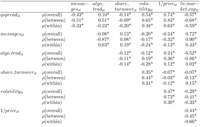
We begin with Table 2, which uses our monthly panel to provide a set of univariate correlations between spreads, algorithmic trading variables, volume, volatility, and share price variables. It is interesting to note that the cross-sectional (between) correlation between spreads andalgo trad_itis positive. This matches the cross-quintile evidence in Figure 1 and Figure 2. This is clearly driven by the cross-section of volume because the correlation with raw message traffic is strongly negative. Perhaps there is a fixed component to message traffic, in that a certain amount of message traffic is required for price discovery regardless of how much trading occurs, giving rise to the positive

cross-sectional correlation between spreads and algo trad_it. While there is undoubtedly value to

further analyzing the causes and effects of cross-sectional variability in algorithmic trading, we focus hereafter on within-stock correlations, because we want to understand the impact of the change in algorithmic trading over time.

The within-stock correlation between quoted spreads and algorithmic trading is negative and significant. This is a contemporaneous correlation, and we do not have anything yet to say about causality. But it appears that, stock by stock in the panel, algorithmic trading is high when spreads are narrow. We also find that algorithmic trading is negatively correlated with volatility, where volatility is measured as the standard deviation of daily midpoint returns for a given month.

2.4

Panel regressions

To confirm that these univariate correlations are robust, we specify regressions for our monthly panel that are of the form:

whereL_it is a liquidity measure (quoted spread, effective spread, or quoted depth) for stocki in montht,A_itis the algorithmic trading measurealgo trad_it, andX_itis a vector of control variables, including trading volume, return volatility, inverse price, and log market cap. Firm fixed effects are always included (α_i); results are always reported with and without calendar fixed effects (γ_t). We estimate separate regressions for each of the market-cap quintiles, and standard errors are robust to general cross-section and time-series heteroskedasticity and within-group autocorrelation (see Arellano and Bond (1991)).

[insert Table 3]

The results are in Table 3 Panel A, and they are qualitatively consistent across the size quintiles. The sign of the algorithmic trading coefficient depends on whether time dummies are included. When there are no calendar fixed effects, the regression is identified using only within-stock variation. Here the results match the univariate within-within-stock correlations: the coefficient on algo trad_it is negative and significant, indicating that an increase in algorithmic trading is associated with narrower quoted or effective spreads. When time dummies are added, changes to common market-wide liquidity factors are removed, and the regression is identified using only idiosyncratic changes in liquidity. Interestingly, the coefficient on algo trad_it changes sign in this case. This does not cast doubt on our other results; it implies only that algorithmic trading and

idiosyncraticliquidity are negatively related. However, it does suggest that the positive time-series association within a given stock between liquidity and algorithmic trading is driven by changes in market-wide common liquidity factors.

If spreads narrow when algorithmic trading increases, it is natural to decompose the spread along the lines of Glosten (1987) to determine whether the narrower spread means less revenue for liquidity providers, smaller gross losses to liquidity demanders, or both. We estimate revenue to liquidity providers using the 5-minute realized spread. The proportional realized spread for thetth

transaction in stockj is defined as:

rspread_jt=q_jt(p_jt−m_j,t+5min)/m_jt, (3)

where p_jt is the trade price, q_jt is the buy-sell indicator (+1 for buys, −1 for sells), m_jt is the midpoint prevailing at the time of thetth trade, andm_j,t+5min is the quote midpoint five minutes after thetth_{trade (the price at which the liquidity provider is assumed able to close her position).}

We measure gross losses to liquidity demanders due to adverse selection using the 5-minute price impact of a trade (adv selection_jt), defined using the same variables as:

Note that there is an arithmetic identity relating the realized spread, the adverse selection (price impact), and the effective spreadespread_jt:

espread_jt =rspread_jt+adv selection_jt. (5)

For these spread components, we estimate panel regressions of the same form as before, and the results are in Panel B of Table 3. Again we report results with and without calendar fixed

effects, but we focus on the results without time dummies. Both realized spreads (espread_jt) and

price impacts (adv selection_jt) are negatively associated with algorithmic trading. More algorith-mic trading is associated with narrower effective spreads, and these narrower spreads imply lower revenue per trade for the liquidity provider as well as smaller gross losses to liquidity demanders. But the relative contributions of the two components are very different. Most of the narrowed spread is due to a decline in adverse selection losses to liquidity demanders. Depending on the size quintile being studied, 75% to 90% of the narrowed spread is due to a smaller price impact. We discuss this in considerable detail below, but we suspect that while manually submitted limit orders are eventually picked off by informed traders, algorithms are better able to avoid some of these informed traders by a so-called “cancel and replace” of the stale limit order.

So far, all we have identified are time-series associations between algorithmic trading and liquidity. We cannot yet say anything about the direction of causality. It is certainly easier to tell a story that goes in the standard direction. For example, algorithmic trading could be providing competition in liquidity provision, thereby improving liquidity. But algorithmic trading is an endogenous choice variable that depends on liquidity, among other parameters. Liquidity is also endogenous and depends on a variety of factors, including the technological and other costs incurred by liquidity providers. Sorting out causality requires an exogenous instrument, and the next section introduces the IV analysis that lies at the heart of the paper.

3

Autoquote

As a result of the reduction of the minimum tick to a penny in early 2001 as part of decimalization, the depth at the inside quote shrank dramatically. In October 2002, the NYSE proposed that a “liquidity quote” for each stock be displayed along with the best bid and offer. The NYSE liquidity quote was designed to provide more information about expressed trading interest at prices outside of the best bid and offer (it was also designed to recapture some of the block trading business that the NYSE had lost to upstairs markets and to algorithms). A liquidity quote was to be a firm bid and offer for substantial size, typically at least 15,000 shares, accessible immediately via a new type

of market order called Institutional Xpress.7

At the time of the liquidity quote proposal, specialists were responsible for manually

disseminating the inside quote.8 Clerks at the specialist posts on the floor of the exchange were

typing rapidly and continuously from open to close and still were barely keeping up with order matching, trade reporting, and quote updating. In order to ease this capacity constraint and free up specialists and clerks to manage a liquidity quote, the exchange proposed to allow the inside quote to be disseminated automatically. Under NYSE Rule 60, display book software would “autoquote” the NYSE’s highest bid or lowest offer whenever there was a change to the limit order book via SuperDOT. This would happen when a better-priced order arrived, when the inside quote was traded with in whole or in part, or when the size of the inside quote changed.

Note that the specialist’s structural advantages were otherwise unaffected by this change. A specialist could still disseminate a manual quote at any time in order to reflect his own trading interest or that of floor traders. Specialists continued to execute most trades manually, and they could still participate in those trades subject to the unchanged NYSE rules. NYSE market share remains unchanged at about 80% around the adoption of autoquote.

[insert Figure 5]

In early 2003, the liquidity quote proposal became enmeshed in a dispute over property rights between the exchange and data vendors such as Bloomberg. The SEC eventually issued a stay delaying the implementation of the liquidity quote, and the liquidity quote did not become operational until June 13, 2003. Meanwhile, the NYSE began to phase in the liquidity quote and autoquote software on January 29, 2003, starting with 6 active, large-cap stocks. During the next two months, over 200 additional stocks were phased in at various dates, and all remaining NYSE stocks were phased in on May 27, 2003. Figure 5 provides some additional details on the phase-in process. The rollout order was determined in late 2002. Early stocks tended to be active large-cap stocks, because the NYSE felt that these stocks would benefit most from the liquidity quote. Beyond that criterion, conversations with those involved at the NYSE indicate that early phase-in stocks were chosen maphase-inly because the specialist assigned to that stock was receptive to new technology. The evidence supports this claim: other than size and trading activity, early phase-in stocks are not significantly correlated with any of the other observables.

Because liquidity quotes were not yet accessible or widely disseminated during this phase-in period, the only change to market structure from January to May 2003 was the non-synchronous addition of autoquote, making this an ideal exogenous event for study. In fact, even when liquidity

7_{For more details, the NYSE proposal is contained in Securities Exchange Act Release No. 47091 (December 23,} 2002), 68 FR 133.

8_{There was one main exception. If a new or cancelled SuperDOT limit order would change the inside quote, the} “Quote Assist” feature of NYSE DisplayBook software automatically disseminated an updated quote after 30 seconds if the specialist had not already done so.

quotes became firm in June 2003, they had little impact on trading. Only a handful of large orders ever used the Institutional Xpress order type, mainly because the spread was typically quite large relative to what could be negotiated in the upstairs market. Most of the information in the liquidity quote was already available to traders and algorithms via NYSE’s Openbook product, which provided periodic snapshots of the NYSE limit order book (see Boehmer, Saar, and Yu (2005) for an analysis of the introduction of OpenBook). Ultimately, liquidity quotes were deemed an unsuccessful innovation and were abandoned in July 2005. But the autoquote feature stayed in place.

For algorithmic traders, autoquote was an important innovation, because it provided much more immediate feedback about the potential terms of trade. Autoquote allowed algorithmic liq-uidity suppliers to, say, quickly notice an abnormally wide inside quote and provide liqliq-uidity ac-cordingly via a limit order. Algorithmic liquidity demanders could quickly access this quote via a conventional market or marketable limit order or by using the NYSE Direct+ facility, which provided automatic execution for limit orders of 1,099 shares or less against the exchange’s dissem-inated quote.

3.1

Autoquote sample

To study the effects of autoquote, we build a daily panel for NYSE common stocks. The sample begins on December 2, 2002, which is approximately two months before the autoquote phase-in begins, and it extends through July 31, 2003, about two months after the last batch of NYSE stocks moves to the autoquote regime. For consistency, we start with the same share price filters as before: stocks with an average share price of less than $5 or more than $1000 are removed. To make our various autoquote analyses comparable, we use the same sample of stocks throughout this section. The Hasbrouck (1991a, 1991b) decomposition (discussed below in section 3.3.2) has the most severe data requirements, so we retain all stocks that have at least 21 trades per day for each day in the eight-month sample period. This leaves 1,082 stocks in the sample.

Stocks are then sorted into quintiles based on market capitalization. Quintile 1 refers to large-cap stocks and quintile 5 corresponds to small-cap stocks. All variables used in the analysis are 99.9% winsorized (that is, values smaller than the 0.05% quantile are set equal to that quantile, and values larger than the 99.95% quantile are set equal to that quantile).

3.2

Autoquote results

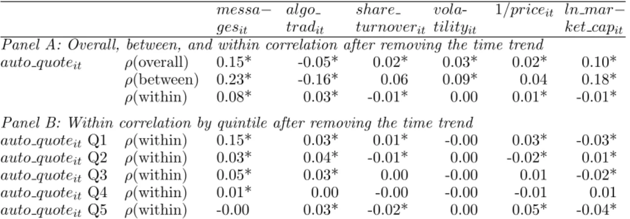
Autoquote clearly leads to greater use of algorithms. Message traffic increases by about 50% in the most active quintile of stocks as autoquote is phased in (see Figure 5); it is certainly hard to imagine that autoquote would change the behavior of humans by anything close to this magnitude. The daily within-stock orrelation between message traffic and the autoquote dummy reported in Table 4 is 0.08. Correlations are higher for large-cap stocks, consistent with the conventional wisdom that algorithmic trading was more effective at the time for active, liquid stocks. Table 4 also shows that there is also a significant positive correlation between the autoquote dummy and our preferred

measure of algorithmic trading algo trad_it, which is the negative of dollar volume (in hundreds)

per electronic message. This plus the exogenous phase-in makes the introduction of autoquote an ideal instrument for assessing the impact of algorithmic liquidity suppliers.9

Within-stock correlations in Table 4 also show that after the introduction of autoquote turnover is higher, volatility is lower, and share prices are higher. However, we have no intention of ascribing these results to autoquote. These results likely reflect the fact that the market rose during the early part of 2003 for unrelated reasons, and they highlight the importance of the staggered introduction of autoquote for cleanly identifying the effect of the market structure change. By including time dummies in the panel specification, we can use non-autoquoted stocks as controls, comparing phased-in autoquoted stocks to not-yet-autoquoted stocks. The time dummies also absorb potential nonstationarity in the time series.10

Our principal goal is to understand the effects of algorithmic liquidity supply on market quality, and so we use the autoquote dummy as an instrument for algorithmic trading in a panel regression framework. Our main instrumental variables specification is a daily panel of 1,082 NYSE stocks over the eight-month sample period spanning the staggered implementation of autoquote. The dependent variable is one of five liquidity measures: the quoted (half) spread, the effective half-spread, the 5-minute realized spread, or the 5-minute price impact of a given trade, all of which are share-volume weighted and measured in basis points, or the quoted depth in thousands of dollars. We have fixed effects for each stock as well as time dummies, and we include share turnover, volatility (measured as the standard deviation of daily midquote returns in percent), the inverse of share price, and the log of market cap as control variables. Results are virtually identical if we exclude these control variables. Based on anecdotal information that algorithmic trading was relatively more important for active large-cap stocks during this time period, we estimate this specification separately for each market-cap quintile.

[insert Table 5]

9_{In the IV regression tables (Tables 5-7), we reportF statistics that reject the null that the instruments do not} enter the first stage regression. We are therefore not concerned about the “weak instruments problem,” also because ourF statistics range from 5.88 to 7.32 and Bound, Jaeger, and Baker (1995, p.446) mention that “F statistics close to 1 should be cause for concern.”

10_{In the IV regression tables (Tables 5-7), we test for any remaining nonstationarity in the residuals through} Dickey-Fuller tests. We reject the null of nonstationarity in all cases.

The results are reported in Panel A of Table 5, and the most reliable effects are in larger stocks. For large-cap stocks (quintiles 1 and 2), the autoquote instrument shows that an increase in algorithmic liquidity supply narrows both the quoted and effective spread. To interpret the estimated coefficient on the algorithmic trading variable, recall that the algorithmic trading

measurealgo trad_it is the negative of dollar volume per electronic message, measured in hundreds

of dollars, while the spread is measured in basis points. Thus, the IV estimate of -0.52 on the algorithmic trading variable for quintile 1 means that an increase in algorithmic trading from the whole-sample mean of $2,634 of volume per message implies that quoted spreads narrow by 0.52 basis points. Over the whole five-year sample interval, the average within-stock standard deviation for algo trad_it is 11.2 or $1,120, so a unit standard deviation change in our algorithmic trading measure is associated with a 5.82 basis point change in proportional spreads.

In the spirit of an event study, we also estimate an analogous non-IV panel regression with the autoquote dummy directly on the right-hand side. We do not report the complete results, but quoted and effective spreads are reliably narrower for the three largest quintiles. For quintile 1, quoted spreads are 0.50 basis points smaller (t = -9.18) after the autoquote introduction, and effective spreads are 0.17 basis points smaller (t = -4.33). Effective spreads narrow even more for quintiles 2 and 3 (0.21 and 0.23 basis points, respectively).

The IV estimate onalgo trad_it is statistically indistinguishable from zero for quintiles 3 through 5. This could be a statistical power issue. Figure 5 shows that most small-cap stocks were phased-in at the very end, reducing the non-synchronicity needed for econometric identification. Perhaps as a result, the autoquote instrument is only weakly correlated with algorithmic trading in these quintiles. Alternatively, it could be that algorithms are less commonly used in these smaller stocks, in which case the introduction of autoquote might have little or no effect on these stocks’ market quality.

Quoted depth also declines with autoquote. One might worry that the narrower quoted spread simply reflects the smaller quoted quantity, casting doubt on whether liquidity actually improves after autoquote is introduced. Here, a calibration exercise is useful. The results for quintile 1 indicate that a one-unit increase in algorithmic trading reduces the quoted spread by 10% (the average quoted spread from Table 1 is 5.31 basis points). The same change reduces the quoted depth by about 4%, based on an average quoted depth of about $92,000. A small liquidity demander is unaffected by the depth reduction and is unambiguously better off with the narrower spread. Consider now a larger liquidity demander who is affected by the depth reduction. She pays 10% less on 96% of her order, and as long as she pays less than a 240% wider spread on the remaining 4% of her order, she is better off overall. Based on the $45.90 average share price for this quintile, the average 5.31 basis point quoted spread translates to 2.4 cents. For these stocks, it seems extremely unlikely that the last 4% of her trade executes at a spread of more than 8.3 cents. Most likely this last 4% would execute one cent wider. This makes it quite clear that the depth

reduction is small relative to the narrowing of the spread.

3.3

Decomposition of the spread improvement

As discussed earlier in the paper, narrower effective spreads imply either less revenue per trade for liquidity providers, smaller gross losses to liquidity demanders, or both. In Table 5 Panel B, we decompose effective spreads into a realized spread component and an adverse selection or price impact component in order to understand the source or sources of the improvement in liquidity under autoquote. IV regressions are repeated using each component of the spread.

The results are somewhat surprising. For quintiles 1 through 3 (large and medium-cap stocks), the realized spread actually increases significantly after autoquote, indicating that liquidity providers are earning greater net revenues. These greater revenues are offset by a larger decline in price impacts, implying that liquidity providers are losing far less to liquidity demanders after autoquote. As before, nothing is significant for the two smallest-cap quintiles.

We describe these results as surprising because they do not match our priors going into the analysis. We thought that if autoquote improved liquidity, it would be because algorithmic liquidity suppliers were low-cost providers who suddenly became better able to compete with the specialist and the floor under autoquote, and thereby improving overall liquidity by reducing aggregate liquidity provider revenues. Instead, it appears that liquidity providers in aggregate were able to capture some of the surplus created by autoquote.

[insert Table 6]

Which liquidity providers benefit? We do not have any trade-by-trade data on the identity of our liquidity providers, but we do know specialist participation rates for each stock each day, so we can see whether autoquote changed the specialist’s liquidity provision market share. We conduct an IV regression with the specialist participation rate on the left-hand side, and the results in Table 6 confirm that, at least for the large-cap quintile of stocks, specialists appear to participate less under autoquote, suggesting that it is other liquidity providers who capture the surplus created by autoquote.

Table 6 also puts a number of other non-spread variables on the LHS of the IV specification. The most interesting is trade size. At least for the two largest quintiles, the autoquote instrument confirms most observers’ strong suspicions that the increase in algorithmic trading is one of the causes of smaller average trade sizes in recent years.

3.3.1 Lin-Sanger-Booth decomposition

The decomposition of the effective spread introduced above has the advantage of being simple, but it also has distinct disadvantages. In particular, it chooses an arbitrary time point in the future (five minutes in this case) and implicitly ignores other trades that might have happened in that five-minute time period. Lin, Sanger, and Booth (Lin, Sanger, and Booth (1995)) develop a spread decomposition model that is estimated trade by trade and accounts for order flow persistence (the empirical fact, first noted by Hasbrouck and Ho (1987), that buyer-initiated trades tend to follow buyer-initiated trades).11 Let

δ=P rob[q_t+1= 1|q_t= 1] =P rob[q_t+1=−1|q_t =−1] (6) be the probability of a continuation (a buy followed by a buy or a sell followed by a sell). Further suppose that the change in the market-maker’s quote midpoint following a trade is given by:

m_t+1−m_t =λ_tq_t. (7) The dollar effective half-spread s_t = q_t(p_t −m_t) and is assumed constant for simplicity. If there is persistence in order flow, the expected transaction price at timet+ 1 does not equal m_t+1 but instead is:

E_t(p_t+1) = δ(m_t+q_t(λ_t+s_t)) + (1−δ)(m_t+q_t(λ_t−s_t)

= m_t+q_t(λ_t+ (2δ−1)s_t). (8)

This expression shows how far prices are expected to permanently move against the market-maker.

While the market-maker earns st initially, in expectation he then loses λ_t + (2δ− 1)s_t due to

adverse selection and order persistence, respectively. Note that this reduces to Glosten (1987)

if δ = 0.5 so that order flow is independent over time. We can identify the adverse selection

component λ by regressing midpoint changes on the buy-sell indicator, and we can identify the

order persistence parameter with a first-order autoregression onq_t. The remaining portion of the

effective spread is revenue for the market maker, referred to by LSB as the fixed component of the spread. Thus, spreads are decomposed into three separate components: a fixed component associated with temporary price changes, an adverse selection component, and a component due to order flow persistence. The fixed, temporary component continues to reflect the net revenues

11_{See Barclay and Hendershott (2004) for discussion of how the Lin, Sanger, and Booth spread decomposition} relates to other spread decomposition models.

to liquidity suppliers after accounting for losses to (the now persistent) liquidity demanders. The adverse selection component captures the immediate gross losses to the current liquidity demander, while the order flow persistence component captures the expected gross losses to those demanding liquidity in the same direction in the near future. We estimate the model and calculate components of the effective spread for each sample stock each day.

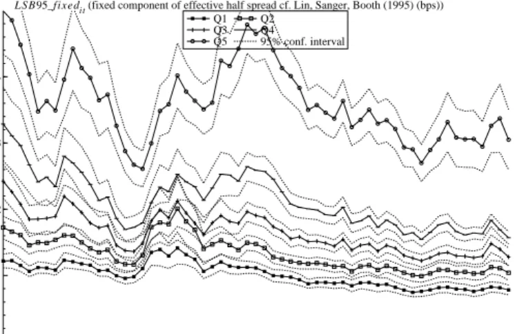
[insert Figure 6]

For each of the market-cap quintiles, the three panels of Figure 6 show how the three LSB spread components evolve over the whole 2001 to 2005 sample period. There are no consistent trends in the fixed component: around the implementation of autoquote, there is an increase for the smallest quintile, but this increase does not extend to the other quintiles. In contrast, the adverse selection component falls sharply during the implementation of autoquote in the first half of 2003. This is true across all five quintiles, and the change appears to be permanent. Beginning in the second half of 2002 and continuing to the end of 2005, there is also a steady decline in the order persistence component of the spread. This suggests less persistence, which could indicate that over this period algorithms and human traders both become more adept at concealing their order flow patterns, perhaps by using mixed order submission strategies that sometimes demand liquidity and sometimes supply it.

[insert Table 7]

As discussed above, we are fortunate and do not need to hang our hats on these time-series declines. The staggered introduction of autoquote allows us to take out all market-wide effects and focus on cross-sectional differences between the stocks that implement autoquote early vs. the stocks that implement autoquote later on. As we did for the simpler decomposition, we can put any one of the LSB spread components on the LHS of our IV specification to determine the sources of the liquidity improvement when there is more algorithmic trading. The results are in Panel A of Table 7 and are quite consistent with the earlier decomposition. For the largest two quintiles, autoquote (and the resulting increases in algorithmic trading) are associated with an increase in the fixed component of the spread, and a decrease in the adverse selection component and the order persistence component. The drop in the adverse selection component is economically quite large. During the autoquote sample period, the within standard deviation in our algorithmic trading variable is 4.54, so a one standard deviation increase in algorithmic trading during this sample period leads to an estimated change in the adverse selection component equal to 4.54∗ −0.26, or about a 1.2 basis point narrowing of the adverse selection component. This is quite substantial, given that the adverse selection component for the biggest quintile is only about 2 basis points on average out of an overall 3.62 basis point effective half-spread. The coefficients on the other two

components are of similar magnitude, indicating similar economic importance. As in the earlier decomposition, there are no significant effects for the smaller-cap quintiles.

3.3.2 Hasbrouck decomposition

While the Lin-Sanger-Booth model begins to consider persistence in order flow, it implicitly limits the form of that persistence to an AR(1) process. Hasbrouck (1991a, 1991b) introduces a VAR-based model that makes almost no structural assumptions about the nature of information or order flow, but instead infers the nature of information and trading from the observed sequence of prices and orders. In this framework, all stock price moves end up assigned to one of two categories: they are either associated or unassociated with a recent trade. Though the model does not make any structural assumptions about the nature of information, we usually refer to price moves as private information-based if they are associated with a recent trade. Price moves that are orthogonal to recent trade arrivals are sometimes considered based on “public information” (examples of this interpretation include Jones, Kaul, and Lipson (1994) and Barclay and Hendershott (2003)).

To separate price moves into trade-related and trade-unrelated components, we construct a VAR with two equations: the first describes the trade-by-trade evolution of the quote midpoint, while the second equation describes the persistence of order flow. Continuing our earlier notation, defineq_jt to be the buy-sell indicator for trade t in stockj (+1 for buys, - 1 for sells), and define

r_jt to be the log return based on the quote midpoint of stockj from trade t−1 to trade t. The

VAR picks up order flow dependence out to 10 lags:

r_t = 10 i=1 α_ir_t−i+ 10 i=0 β_iq_t−i+_rt, (9) q_t = 10 i=1 γ_ir_t−i+ 10 i=1 φ_iq_t−i+_qt, (10)

where the stock subscripts j are suppressed from here on. The VAR is inverted to get the VMA

representation: y_t = r_t q_t =θ(L)_t = a(L) b(L) c(L) d(L) _{rt qt} , (11)

where a(L), b(L), c(L), andd(L) are lag polynomial operators. The permanent effect on price of an innovation et is given bya(L)_rt+b(L)_qt , and because we include contemporaneousq_t in the return equation,cov(_rt, _qt) = 0 and the variance of this random-walk component can be written

as: σ_w2 = ( ∞ i=0 a_i)2σ_r2+ ( ∞ i=0 b_i)2σ2_q, (12)

where the second term captures the component of price discovery that is related to trade, and the first term captures price changes that are unrelated to trading (sometimes referred to as public information). As discussed in Hasbrouck (1991a, 1991b), this method is robust to price discreteness, lagged adjustment to information, and lagged adjustment to trades.

[insert Figure 7]

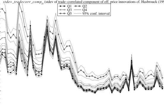
The VAR and the trade-related and non-trade-related standard deviations are estimated for each stock each day. We calculate monthly averages for each quintile during the autoquote sample period and graph these in Figure 7. The most striking feature of the graph is the decline in the trade-related standard deviation, while the non-trade-related standard deviations do not change much as autoquote is introduced. This indicates that under autoquote much more information is being incorporated into prices without trade, consistent with the results in Boulatov and George (2007) when informed traders compete via limit orders.

While these time-series effects appear large, again we prefer to identify the effect using the staggered autoquote instrument. The IV panel regression is estimated first with the daily trade-related standard deviation as the dependent variable. We then repeat using the non-trade-trade-related standard deviation on the left-hand side. The panel regressions continue to include stock fixed effects, calendar dummies, and the same set of control variables.

The results can be found in Panel B of Table 7, and at least for the two larges quintiles they confirm that the time-series graphs are not spurious. Consistent with other methodologies, we do not find consistently reliable effects for the three smallest-cap quintiles.

When a large-cap stock adopts autoquote and experiences an exogenous increase in algo-rithmic trading, there is much less trade-correlated price discovery, and much more price discovery that is uncorrelated with trading. We discuss this further below, but it seems likely that algorithms are responding quickly to order flow information and price moves of this and other stocks, thereby updating quotes to prevent them from becoming stale and being picked off.

Based on our estimates, algorithmic trading has an economically important effect on the nature of price discovery. During the autoquote sample period, the within standard deviation in our algorithmic trading variable is 4.54, so a one standard deviation increase in algorithmic trading during this sample period leads to an estimated change in trade-correlated price discovery equal to 4.54∗ −0.22, or almost exactly a 1 basis point reduction in the standard deviation of trade-correlated returns. Figure 7 shows that this is the same order of magnitude as the actual level of trade-correlated standard deviations measured from trade to trade, so this is indeed a substantial

change in how prices are updated to reflect new information over time.

4

Discussion and interpretation

To help make sense of our counter-intuitive results (particularly the realized spread or temporary component results), we turn next to a very simple generalized Roll model that is a slight variation on one developed in Hasbrouck (2007). Though the model is quite simple, it provides a useful framework for thinking about algorithmic trading and delivers a number of empirical predictions, all of which match our empirical results.

4.1

A generalized Roll model

The “game” has two periods, each with an i.i.d. innovation in the efficient price:

m_t =m_t−1+w_t, (13)

wherew_t ∈ {,−}, each with probability 0.5. The game features three stages:

- At t = 0, risk-neutral humans can submit a bid and ask quote and, given full competition, the first one arriving bids her reservation price.

- At t = 1, humans can buy the information w₁ at cost c. If they buy the information, they

can submit a new limit order.

- At t = 2, two informed liquidity demanders arrive, one with a positive private value associated with a trade, +θ, the other with a negative private value, -θ.

We assume that 2c > θ, i.e., the cost of “observing” information for humans is sufficiently

high that they do not update their quotes. The technical assumption > θ ensures that trade

occurs only if there is non-zero private information att= 2, and that only one of the two arriving liquidity demanders transacts in that case.

m

m

m

m

m

m

A

A

B

B

ε

There are four equally likely paths through the binomial tree: _{uu, ud, du}, and _dd, where

urepresents a positive increment of to the fundamental value and_d is a negative increment. In

equilibrium, humans do not buy thew₁ information and update the quote att= 1, since they have

to quote so far away from the efficient price to make up for c that neither liquidity demander will transact at that quote (as 2c > θ). Given that they do not acquire the w₁ information, humans protect themselves by setting the bid price equal to m₀−2 and the ask price equal to m₀+ 2. One of the liquidity demanders trades att= 2 if the path is either_uu or_dd; the quote providers break even. If the path is_udor_du, then there is no trade, because the liquidity demander’s private value is too small relative to the spread.

Clearly, under these assumptions all price changes are associated with order flow, and there is no public information component.

4.1.1 The model with algorithmic trading

m

m

m

m

A

A

B

B

θ

Now we introduce an algorithm that can buy the w₁ information at zero cost (c = 0).

The results at t= 0 remain unchanged. Att= 1, the algorithm optimally issues a new quote. To

illustrate the idea, suppose w₁ > 0. The algorithm knows that it is the only liquidity provider in possession ofw₁, and so it puts in a new bid equal tom₀−θ. Ifw₂>0 as well, then a transaction

takes place at the original ask of m₀ + 2. If w₂ < 0, then a liquidity demander will hit the algorithm’s bid. This bid is below the efficient price, so there will eventually be a reversal, and there is a temporary component in prices. Contrariwise, ifw₁ <0, the algorithm places a new ask atm₀+θ, which is traded with if it turns out thatw₂>0.

In the presence of algorithmic trading, part of the change in the efficient price is revealed through a quote update without trade. Public information now accounts for a portion of price discovery, and imputed revenue to liquidity suppliers is now positive. Thus, the model can explain even the surprising empirical findings on realized spreads and trade-correlated price moves. The model also delivers narrower quoted spreads and more frequent trades, both of which are also observed in the data.

To deliver an increase in realized spread, it is important in the model that competition between algorithms be less vigorous than the competition between humans. This seems plausible in reality as well. As autoquote was implemented in 2003, the extant algorithms might have found themselves with a distinct competitive advantage in trading in response to the increased information flow, given that new algorithms take considerable time to build and test.

What kind of information can algorithms efficiently observe? There are probably many answers, but it is hard to tell, given the general opacity practiced by algorithm providers and users. Nevertheless, we suspect that two kinds of information are of first-order importance. First, we think algorithms can easily take into account common factor price information and adjust trading and quoting accordingly. For example, if there is upward shock to the S&P futures price, an algorithmic liquidity supplier in IBM that currently represents the inside offer may decide to cancel its existing sell order before it is picked off by an index arbitrageur or another trade, replace the sell order with a higher-priced ask. Shocks to other stocks in the same industry could cause similar reactions from algorithms. Second, some algorithms are designed to sniff out other algorithms or otherwise identify order flow and other information patterns in the data. For example, if an algorithm identifies a sequence of buys in the data and concludes that more buys are coming, an algorithmic liquidity supplier might adjust its ask price upward. Information in newswires can even be parsed electronically in order to adjust trading algorithms.12

4.2

Alternative explanations

Up to now, we have focused on the algorithmic trading channel, but it is important to consider whether a more mechanical explanation might account for our autoquote results. What might we expect if autoquote simply makes quotes less stale and has no other effects? It turns out that if this is the only effect of autoquote, we would expect to see effective spreads widen once autoquote

is turned on.

To see this, let a_t and b_t be the ask and bid prices at time t, and assume this quote is disseminated by the specialist. Limit orders arrive or are cancelled, and at a later timet, a_t and

b_t are the best ask and bid prices. Assume thata_t andb_t are disseminated only after the adoption

of autoquote; otherwise, the econometrician identifiesa_t andb_t as the ask and bid in effect at time

t.

To simplify the exposition, assume that the ask side of the book changes (a_t =a_t) while

the bid side of the book remains unchanged (b_t = b_t). Symmetric arguments apply for changes

to the bid side of the book alone, and the results also hold when both the bid and the ask change betweentandt.

There are two possibilities for the change in the inside ask. If the time t inside ask is

cancelled, then a_t > a_t. If instead a new sell order arrives at time t that would improve the

inside quote, then a_t < a_t. Overall, if cancels are more common than improvements, then prior to the adoption of autoquote the disseminated quoted spread is artificially narrow, and autoquote should be associated with a widening of quoted spreads. However, we find the reverse. Autoquote is associated with a narrowing of the quoted spread, so we focus hereafter on the arrival of new orders at timet that improve the existing time t quote. Prior to autoquote, we continue to observe the old, wider quote (a_t, b_t) at time t. Under autoquote, the new, narrower quote (a_t, b_t) is

disseminated at timet.

Let m_t = 1/2(a_t + b_t) be the midquote at time t. Under autoquote, we see the true

state of the order book, and if a trade at timet occurs at price p_t (at either the bid priceb_t or

the ask price a_t), assume that the effective half-spread s_t = q_t(p_t - m_t) is correctly measured.

In contrast, before the adoption of autoquote the observed midquote at timet ism_t = 1/2(a_t +

b_t), which is stale. Because we focus on the arrival of a sell order that improves the ask,m_t < m_t,

which means that in the absence of autoquote the observed quote midpoint is biased upwards. Define the measured effective spread pre-autoquote ass_t,pre = q_t(p_t -m_t).

Thus, the change in the measured effective spread under autoquote is the difference s_t

-s_t,pre = q_t (m_t - m_t) = q_t (a_t - a_t)/2. The term in parentheses is positive, since the arriving

sell order improves the quote by lowering the ask price, so the effective spread declines under

autoquote if and only if E(q_t) < 0. But this cannot be the case as long as the demand for

immediacy is downward sloping in the price of immediacy. To say it another way, a better ask price should on average draw in a marketable buy order, which implies E(q_t)>0. Thus, if autoquote is simply displaying quotes that were previously undisseminated, the result should be a widening of the effective spread under autoquote.

Note that there is an implicit assumption in the above analysis that without autoquote,

q_t, the sign of the trade. The trade sign can indeed be affected if the new ask pricea_t is below the

disseminated midquotem_t. In this case both the true ask and bid prices are below the disseminated midquote, and with the right choice of parameter values effective spreads could be mechanically narrower under autoquote. However, this scenario seems unlikely to dominate. First, it is quite likely that the specialist would disseminate an updated quote if an incoming limit order crosses the midquote in this way, as the new quoted spread would be less than half as wide as the old quoted spread. Second, if this scenario were empirically important, the resulting trade-signing errors would bias downward the pre-autoquote estimates of the adverse selection component of the spread, because future price changes would be less correlated with trade signs. In this scenario,

we would expect to see an_increase in adverse selection with the elimination of stale quotes under

autoquote. This is the opposite of our findings in Tables 5 and 7.

To summarize, a mechanical increase in quote disseminations would almost surely work against us, widening the effective spread. Thus, the elimination of stale quotes is unlikely to be the source of our results.

5

Conclusions

The declining costs of technology have led to its widespread adoption throughout financial indus-tries. The resulting technological change has revolutionized financial markets and the way financial assets are traded. Many institutions now trade via algorithms, and we study whether algorithmic trading at the NYSE improves liquidity. Using panel regressions over the five years following deci-malization, we establish that time-series increases in algorithmic trading are associated with more liquid markets. To establish causality we use the staggered introduction of a structural change at the NYSE (autoquoting) as an exogenous instrument for algorithmic trading. We demonstrate that increased algorithmic trading lowers adverse selection and decreases the amount of price dis-covery that is correlated with trading. These results suggest that algorithmic trading lowers the costs of trading and increases the informativeness of quotes and prices. Surprisingly, the revenues to liquidity suppliers also increase with algorithmic trading. This is consistent with algorithmic liquidity suppliers having market power as they introduce their algorithms.

We have not studied it here, but it seems likely that algorithmic trading can also improve linkages between markets, generating positive spillover effects in these other markets. For example, when computer-driven trading is made easier, stock index futures and underlying share prices are likely to track each other more closely. Similarly, liquidity and price efficiency in equity options probably improves as the underlying share price becomes more informative.

One caveat is in order, however. Our overall sample period covers a period of generally rising stock prices, and stock markets are fairly quiescent during the 2003 introduction of autoquote.