No. 11-2010
Do Capital Inflows Hinder Competitiveness?
The Real Exchange Rate in Ethiopia
Pedro M. G. Martins
Institute of Development Studies (IDS) University of Sussex
pedromgmartins@gmail.com
Abstract:
This paper investigates the determinants of the real exchange rate (RER) in Ethiopia. In particular, it assesses whether large capital inflows (e.g. foreign aid and remittances) have an impact on the RER. This empirical exercise tries to improve the current literature in a number of ways: (i) the use of quarterly data provides a larger sample size and enables the modelling of important intra-year dynamics, which should lead to better model specifications; (ii) the use of several cointegration approaches allows interesting methodological comparisons; and (iii) the use of a time series model (Unobserved Components) provides a new empirical approach and a robustness check on the econometric models. The results suggest two main (long-run) determinants of the RER in Ethiopia: trade openness is found to be correlated with RER depreciations, while a positive shock to the terms of trade tends to appreciate the RER. Foreign aid is not found to have a statistically significant impact, while there is only weak evidence that workers’ remittances could be associated with RER appreciations. The lack of empirical support for the Dutch disease hypothesis suggests that Ethiopia has been able to effectively manage large capital inflows, thus avoiding major episodes ofmacroeconomic instability.
JEL Classification:
C22, F35, O24, O55Key Words:
Real Exchange Rate, Foreign Aid, Time Series Models, Africa
This paper is based on the author’s DPhil research, which was financially supported by theFundação para a Ciência e a Tecnologia. The author would also like to thank the comments and suggestions from the participants of the attendants of an IDS-Sussex seminar in 2009.
1. Introduction
The term ‘Dutch disease’ is commonly used to describe the potential negative effects of large inflows of foreign currency on the recipient economy.1This ‘disease’ usually manifests itself through the appreciation of the real exchange rate and the consequent loss of export
competitiveness. The surge in foreign exchange often takes the form of higher export receipts (e.g. following an increase in natural resource prices), foreign direct investment, workers’ remittances or foreign aid inflows. The main focus of this paper will be on the latter two.
The real exchange rate is one important channel through which foreign aid inflows can affect the recipient economy. Concerns about ‘Dutch disease’ have been recently revived due to the commitment of the international development community to scale up aid flows to developing countries, and in particular to double the resources to Africa. Evidence that foreign aid has had a detrimental effect on the growth of the export sector could offer an explanation for the difficulty of finding robust evidence that aid fosters economic growth. For example,Rajan
and Subramanian (2005)argue that aid flows are responsible for the decline in the share of labour intensive and tradable industries in the manufacturing sector – through its contribution to real exchange rate overvaluation.2However, the empirical evidence is mixed, with several studies even suggesting that foreign aid leads to the depreciation of the local currency, potentially through supply side effects or aid tied to imports(Li and Rowe, 2007:17).
Moreover, the impact of foreign aid on the composition of (public) expenditure seems to be crucial to the overall effect on the exchange rate. If aid inflows are used to purchase capital goods from abroad (e.g. import support), then they are not likely to have a significant impact on the local currency. However, if the inflows are significantly biased towards the purchase of (non-tradable) local goods, and if there are significant supply-side constraints, then rising domestic inflation will erode the real exchange rate, affecting the competitiveness of the country’s exports. These are some of the effects that this empirical exercise will try to uncover in order to improve our understanding of how large aid inflows impact economic performance.
The paper is organised in seven sections. After this short introduction, the theoretical underpinnings of this study will be presented. Section 3 reviews and summarises the
1The term was originally coined byThe Economistto reflect the paradoxical impact of the discovery of natural gas deposits
in the North Sea on the Dutch manufacturing sector, through the appreciation of the Dutch real exchange rate.
empirical evidence from the ‘Dutch disease’ literature. Section 4 introduces the
methodologies to be used in this study, while section 5 draws some considerations about the data. Section 6 presents the empirical results from the econometric models and the structural time series model. Section 7 concludes the paper.
2. Theoretical Background
2.1 Core Dutch Disease Model
This section deals with the theoretical arguments and predictions of the Dutch disease literature. The core model is described inCorden and Neary (1982:826). Their framework assumes a small open economy with three sectors: (i) the booming export sector (e.g. energy); (ii) the lagging export sector (e.g. manufacturing); and (iii) the non-traded goods sector (e.g. services), which supplies the domestic economy. The price of the non-traded good adjusts to equal supply and demand, in contrast to the export sectors where exogenous world prices prevail. The authors describe two main effects of an export sector boom: (i) spending effect; and (ii) resource movement effect. To better understand thespending effect, assume that the energy sector does not use any labour. The energy boom will entail higher export earnings and thus higher foreign exchange inflows. It is unlikely that all this extra income will be spent on imports, thus the boom will have an impact on the domestic
economy. Provided that the demand for non-tradables rises with income, the boom will create excess demand in the non-tradable sector, increasing their price and leading to real exchange rate appreciation.3Turning to theresource movement effect, assume that the income-elasticity of demand for non-tradables is zero. The increased marginal productivity of labour in the booming export sector raises profitability and the demand for labour in the energy sector. This will push wages up and eventually induce a relocation of labour to the booming sector at the expense of the other two. The fall in employment in the manufacturing sector will
contract output (‘direct deindustrialization’) and the higher price of non-traded goods leads to real exchange rate appreciation. Through these two effects the authors suggest that the
traditional export sector is crowded-out by the other two sectors(Ebrahim-zadeh, 2003). This core model can be adapted to understand the potential impact of a surge in aid inflows, rather than an energy boom(Nkusu, 2004:9).4Foreign aid can be seen as a real income transfer that will raise the demand for both tradable and non-tradable goods produced in the
3
The price of traded goods in the world market remains unchanged (small economy assumption).
economy. In the context of a small open economy, the increase in the demand of tradable goods will not affect their prices, since these are exogenously determined in world markets. However, the increased demand for non-tradable goods will place an upward pressure on prices, hence, the real exchange rate appreciates (spending effect). The profits of exporters are squeezed as the prices for domestic inputs (services, labour, etc.) increase, therefore
discouraging the production of tradable goods. Meanwhile, the relative incomes of producers of non-tradable goods are increased.
The appreciation of the RER will materialise regardless of the exchange rate regime. In a
flexible exchange rate regime, an increase in aid inflows will appreciate the nominal exchange rate as foreign currency is swapped for domestic currency. This appreciation will reduce the value of exports in local currency, which will reduce profitability if production costs such as wages are not adjusted downwards. In afixed exchange rate regime, aid flows will push up the price of domestically produced goods that are in short supply. In both cases, the aid surge will induce an appreciation of the real exchange rate, thus hindering the
development of the tradable sector of the economy.
Furthermore, there is also aresource movement effect. The increased demand for non-traded goods will push wages up in the sector, bidding labour out of the tradable goods sector – where wages cannot be increased without squeezing the profits. As the marginal product of labour and wages in the non-tradable sector increase, there will be an incentive to relocate labour from the (lagging) tradable sector to the non-tradable sector. The final effect will depend on the factor intensity of the sectors.
Despite the popularity of the arguments presented above, the empirical support for Dutch disease effects has been mixed, especially with regard to aid inflows (as will be demonstrated in section 3). This apparent disagreement between theory and empirical evidence is bridged byNkusu (2004). The author provides a modified theoretical framework to show that, under certain circumstances, Dutch disease symptoms may not materialise. He uses a Salter-Swan framework with two sectors to illustrate the importance of two crucial assumptions of the core Dutch disease model: (i) full and efficient employment of production factors (i.e. countries produce on their production possibility frontier) and, (ii) perfectly elastic demand for tradables (small-country assumption).
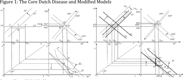
The figure below presents the core Dutch disease model (left panel) and Nkusu’s modifications (right panel). The top-left quadrant of each panel represents the tradables market –PTis the price andTthe quantity – while the top-right quadrant illustrates the market for non-tradables. Moreover, the bottom-right quadrant presents the production possibility frontier (PPF). The left panel provides the setting for the core Dutch disease model. The small-country assumption is reflected on the perfectly elastic demand for tradables (horizontalDT), thereby making its price exogenous. The trade balance is in equilibrium (C). In addition, the country produces and consumes on the PPF (B). Hence, a large inflow of foreign aid will increase the demand for non-tradables (DNTtoDNT’) and its price (PNTtoPNT’). Since the price of tradables (PT) remains at the same level, the RER will increase and discourage the production of tradables. This is usually referred to as the
spending effect. Furthermore, the consequent increase in the supply of non-tradables (SNTto
SNT’) will occur at the cost of the tradables sector, which contracts fromSTtoST’. This is theresource movement effect, which is mainly due to the relocation of labour to the non-tradables sector.Nkusu (2004)also makes reference to anexpenditure-switching effect, which is a disincentive to buy non-tradables due to the RER appreciation. The increase in income (Y
toY’’) and the shift from indifference curveIDtoID’will be consistent with a higher demand for tradables, which will create a trade deficit of magnitudeC’C’’.
Figure 1: The Core Dutch Disease and Modified Models
Source:Nkusu (2004:9&12)
Nkusu (2004)proposes two modifications to the core Dutch disease model. Firstly, he argues that many low-income countries (LICs) produce below their potential, and not on the PPF. On the right panel, the country produces atA(within the PPF) and consumes atB. The PPF assumption is synonymous of full-employment and efficient use of the production factors,
which is clearly not the case for many LICs suffering from supply-side constraints – high structural unemployment and inefficient use of production factors seems a more plausible assumption. By relaxing this assumption, the extra demand for non-tradable goods brought by aid flows can be accommodated without creating inflationary pressures (especially if aid flows are used to improve productivity).
Secondly, he argues that the small-country assumption is not realistic with regard to many domestically produced importables in LICs. The assumption states that the price of tradable goods is exogenously determined, and hence a surge in aid will place upward pressures on wages, squeezing out profits. However, the author argues that the threat of
de-industrialisation is mitigated in LICs where there is imperfect substitutability between
domestically produced manufactured goods and imported ones. The imperfect substitutability allows domestic manufacturers to raise prices and increase supply in response to domestic market conditions, such as increased demand, regardless of whether they use imported or domestically produced inputs. Therefore, the demand of tradable goods is represented by a downward-sloping curve (DT). The total supply of tradables (ST) includes home supply (Hst)
and imports equivalent to the trade deficit (TD). The initial dynamic impact of an increase in aid inflows is similar to the core model. The increase in the demand for non-tradables (DNT), and its respective price (PNT’), leads to an increase in supply (SNT). The country now
produces atA’(on the PPF) and consumes atB’’. In the modified version, however, the supply of tradables is actually increased (no ‘de-industrialisation’), the RER may not appreciate, and the trade balance can be improved.
In summary,Nkusu (2004)suggests that if low-income countries (LICs) can “draw on their idle productive capacity to satisfy the aid-induced increased demand”, the appreciation of the exchange rate will be negligible. His theoretical contribution seems to explain why Dutch disease symptoms are not necessarily present in episodes of resource boom and aid surges.5 This line of investigation has been taken up by several calibrated general equilibrium models, as described in section 3.
5
Moreover,Torvik (2001)uses a learning-by-doing model (with spillovers between the sectors) to show that, in the long-run, a ‘foreign exchange gift’ induces a real exchange rate depreciation.
2.2 Determinants of the Real Exchange Rate
The exchange rate is a critical price for an open economy. The exchange rate affects the volume of both imports and exports (by changing their relative prices), as well as the stock of foreign debt in domestic currency terms. In fact, all transactions with the rest of the world can be potentially affected by the level of the exchange rate. A depreciation of the exchange rate is often associated with competitiveness gains, in the sense that the relative price of exports will fall, therefore becoming more attractive to foreign importers. Since imports become relatively more expensive, we usually observe an improvement of the trade balance.6
However, since the stock of foreign debt becomes more expensive in local currency, currency depreciations usually worsen a country’s debt position and increase interest payments.
Moreover, foreign direct investments may benefit from relatively cheaper domestic goods, but revenues in local currency will translate into less foreign currency to repatriate. Finally, foreign aid flows will be able to purchase more domestic goods than before. In addition to the large literature on the merits and shortcomings of devaluations, there is an understanding that excess exchange rate volatility and misalignment can have substantial negative welfare effects. It is therefore not surprising that there is a vast literature trying to uncover the main determinants of the real exchange rate, in order to improve exchange rate policies.
There are two main approaches to understand the behaviour of the real exchange rate (RER). The traditional approach is based on the Purchasing Power Parity (PPP) theory, which defines the RER as the nominal exchange rate corrected by the ratio of the foreign price level to the domestic price level (purchasing power):
whereP*andPare foreign and domestic prices, respectively, and the NER is expressed as units of domestic currency per unit of foreign currency. Therefore, a rise [fall] in the RER represents a depreciation [appreciation] of the domestic currency. Depending on the price indices used in the computations, the RER can be seen as the relative price of foreign to domestic consumption or production baskets(Edwards, 1989:5).
6
Provided that the Marshall-Lerner condition is met, i.e. the sum of the absolute export and import price elasticities is greater than unity.
The absolute PPP equilibrium condition for a pair of currencies is achieved when the nominal rate ensures that the domestic purchasing powers of the currencies are equivalent. This
implies that the RERPPPis equal to 1.
Hence, the PPP theory is grounded on the law of one price, which suggests that market forces acting on either the prices or the NER (depending on the exchange rate regime) will ensure that relative prices equalise across countries or at least that we have negligible price
differentials(Hallwood and MacDonald, 2000:122). Empirically, it is assumed that this PPP relation holds in the long-run with strong mean reversion (stationarity). Another consequence of this approach is that the equilibrium real exchange rate (ERER) is given by a scalar
(constant), which is assumed to hold for the entire period. The equilibrium value is often found by looking at the RER for a relative stable period, when external equilibrium was likely to hold. One way to empirically test this hypothesis is to use regression analysis on the following equation:7
If absolute PPP holds, then1=1,2=–1 andα=0. However, empirical work has often found
little evidence of the validity of this relationship. Movements outside the ‘equilibrium’ appear to be persistent, indicating that mean reversion is slow (PPP relation is non-stationary). Hence, the effects of a shock take too long to disappear, which is not compatible with the ‘arbitrage condition’ (i.e. law of one price). This ‘PPP puzzle’(Rogoff, 1996)can be
explained by a number of reasons. Trade barriers (in the form of quantitative restrictions or taxes), transaction costs and productivity gains are amongst the factors that are likely to influence the path of the RER, thus it is unlikely that a single value of the RER can be seen as ‘equilibrium’.
The weaker version of the PPP (relative PPP) accepts that due to market imperfections the relationship may not hold. Instead, this hypothesis states that the percentage change in the NER will equal the inflation differential (in the equation below,3=1 and4=–1). Hence, an
increase in relative prices will force the NER to depreciate (law of one price). However, it should be noted that this theory requires that factors such as trade barriers and transaction costs remain constant through time, an assumption that is not likely to hold. In fact, there has been only weak support for this hypothesis.
This paper uses an alternative approach to the PPP theory. The equilibrium real exchange rate (ERER) is defined byEdwards (1989:5&8)as the domestic relative price of tradable goods to non-tradable goods that simultaneously attains internal and external equilibrium:
wherePTis the price of tradables (expressed in local currency) andPNTthe price of
non-tradables. Internal equilibrium is defined as the clearing of the non-tradable goods market, hence with employment at the ‘natural’ level. External equilibrium is achieved when current account balances are compatible with long-run sustainable capital flows. This definition implies that the ERER is not a constant number, as it depends on a number of real and nominal determinants. It is also important to distinguish between the short-run and the long-run, since some determinants may only have a temporary impact on the ERER. Misalignment is defined as “sustained departures of the actual real exchange rate from its [long-run]
equilibrium level”(Edwards, 1989:15). For example, during the 1980s several developing countries had overvalued real exchange rates.
Edwards (1989)constructs a benchmark intertemporal general equilibrium model to analyse the theoretical impact of a number of real disturbances on the ERER. The assessment suggests that an increase in tariffs (trade protectionism) will usually generate an equilibrium real appreciation, while a relaxation of exchange controls (capital account liberalisation) will induce an initial equilibrium real depreciation. Transfers from abroad (e.g. foreign aid) will always result in ERER appreciation. The total effect of other determinants is ambiguous. For example, a worsening of the terms of trade will result in ERER depreciation if the income effect dominates the substitution effect, while the impact of government consumption will
7
depend on its composition – if mainly tradables, then depreciation will ensue. Finally, the impact of technological progress will depend on how the demand (income) and supply effects play out.
3 Literature Review
Notwithstanding the theoretical arguments put forward byCorden and Neary (1982),Corden
(1984),van Wijnbergen (1984, 1986)8andEdwards (1989), it is has been difficult to establish a robust association between increased aid inflows and the appreciation of the real exchange rate. This section provides an overview of the evidence on the Dutch disease, with special reference to foreign aid inflows. It starts with a brief presentation of the findings of computable general equilibrium (CGE) studies, followed by a survey of the empirical evidence from both cross-country and time series econometrics.9
Computable General Equilibrium
Computable general equilibrium (CGE) models are a useful tool to explore the different dynamics and transmission channels surrounding the Dutch disease hypothesis.10Vos (1998) finds that foreign aid inflows induce strong Dutch disease effects in Pakistan, although these symptoms can be mitigated if the flows are used to alleviate investment constraints in the production of traded goods. He also argues that, based on similar models for Mexico, the Philippines and Thailand, the findings for Pakistan are not “easily generalisible and depend strongly on the existing economic structure, investment and savings behaviour of institutional agents, and the allocation of additional capital flows among public and private sector agents.”
Bandara (1991:92)also highlights the fact that the standard Dutch disease results depend, to some extent, on the model assumptions, parameter values, and model closure. Moreover,
Benjamin (1990)demonstrates that despite the RER appreciation, the tradable sector (manufacturing) only contracts in the short-run, consequently expanding via new
investments.Laplagne et al (2001)calibrate a CGE for a typical South Pacific microstate and also find evidence of Dutch disease effects, in particular of the relative contraction of the tradables sector.Collier and Gunning (1992)suggest that foreign aid inflows tend to inhibit
8van Wijnbergen (1984:53)
argues that Dutch disease is a ‘disease’ because “corrective medicine is needed”.
9
CGE simulations do not provide empirical tests of the Dutch Disease hypothesis. However, they can offer insights into the potential size of such effects, provided that the model is a reliable representation of the economy under consideration.
10
Some studies focus on mitigating policy responses rather than testing the empirical validity of such effects, which are often built-in by construction or dependent on crucial assumptions about the structure of the economy.
the export supply response to liberalisation through a spending effect (relocation of investment and labour into non-tradables).
Over the last couple of years there has been a renewed interest in the subject, partly due to
donor commitments to scale up aid resources to developing economies.Adam and Bevan
(2006)develop a small dynamic CGE model (calibrated for Uganda) with learning-by-doing externalities where investment in public infrastructure creates an intertemporal productivity spillover. Their simulations show that the supply-side effects of aid-financed public
expenditure can outweigh the short-run (demand-side) Dutch disease symptoms, especially if these investments are biased towards the non-tradable sector – therefore increasing the
productivity of private factors in the production of domestic goods.Devarajan et al (2008)use
a standard neoclassical growth model, based on the Salter-Swan open-economy framework.11
They suggest that concerns of Dutch disease do not materialise if recipients are able to
optimally plan consumption and investment over time, a result that is valid for permanent and temporary aid shocks, while not requiring “extreme assumptions or additional productivity story.” However, Dutch disease might become a concern if aid flows are disbursed in an unpredictable or volatile fashion (affecting intertemporal smoothing). Hence, they conclude that “any unfavourable macroeconomic dynamics of scaled-up aid are the result of donor behaviour rather than the functioning of recipient economies.”Cerra et al (2008)use a dynamic dependent-economy model to show that while untied aid causes a temporary (and small) appreciation of the real exchange rate in the short-run, it does not induce Dutch disease effects in the long-run (i.e. no relative price effects), as long as capital is perfectly mobile between sectors.12In contrast, tied aid will cause permanent relative price changes, but the effects will depend on the sectoral allocation of aid: aid flows directed to enhancing productivity in the traded sector will lead to an appreciation of the real exchange rate (Balassa-Samuelson effect), while if directed to the non-traded sector they will lead to a depreciation.
Finally, some studies focus their attention on macroeconomic management policies that have the potential to mitigate the undesirable effects of aid inflows, such as RER appreciation and volatile expenditure patterns.Prati and Tressel (2006)investigate optimal fiscal and monetary policy responses in the context of a model with a closed capital account and
learning-by-11
The model uses data from Madagascar, Mozambique, and the Philippines.
doing externalities, where foreign aid inflows impact productivity growth through (positive) public expenditure and (negative) Dutch disease effects. They argue that although foreign aid inflows have a negative impact on exports, this effect can be undone by tighter
macroeconomic policies. This is achieved through the reduction of the net domestic assets of the central bank (‘sterilisation’), which reflects both monetary and fiscal policies. This policy can be effective in preventing RER appreciation when aid is excessively ‘front-loaded’ (when Dutch disease costs are higher than expenditure and productivity benefits), and thus the economy is better-off saving part of the aid flows for future use. Nonetheless, when foreign aid is excessively ‘back-loaded’ expansionary policies can improve welfare if the stock of international reserves is large enough. Similarly,Buffie et al (2008, 2004)use an intertemporal optimising model to investigate the monetary and exchange rate policy options available to countries facing persistent shocks to aid flows. They conclude that a ‘pure float’ regime performs very poorly (RER overshoots), while in a ‘crawling peg’ regime inflation increases in the short-run. Bond sterilisation will control inflation, but the interest burden will rise. The preferred scenario is a ‘managed float’, where the central bank “uses unsterilised foreign exchange intervention to target the modest real appreciation needed to absorb the aid inflow.” This scenario ensures low real interest rates and a quick macroeconomic adjustment,
challenging suggestions that the expansion of domestic liquidity brought by aid flows requires a combination of sterilisation and a free float.
In conclusion, the CGE literature seems to suggest that while Dutch disease remains a concern for macroeconomic management in the short-run, these negative effects can be mitigated, or even reversed, if foreign aid flows induce positive supply-side effects. Moreover, there are a number of policy tools that can be deployed in order to mitigate the potentially pervasive effects of a windfall of foreign aid. The challenge for empirical
econometric studies is to assess whether there is robust evidence of Dutch disease effects, or if these are undone (or at least mitigated) through appropriate macroeconomic policies (e.g. fiscal and exchange rate).
Cross-Country
Most of the empirical studies reviewed in this sub-section use single-equation panel data regressions. Recent works have used dynamic panel data techniques, while one study has employed cointegration analysis.Adenauer and Vagassky (1998)use a panel of four CFA Franc Zone countries (Burkina Faso, Côte d’Ivoire, Senegal and Togo) to estimate the impact
of foreign aid flows on the RER. Their GLS results suggest that both foreign aid and the terms of trade are correlated with RER appreciations. Moreover, real GDP and a proxy for technological differentials13were not statistically significant.Ouattara and Strobl (2004) expand the previous analysis to 12 countries of the CFA Franc Zone and obtain quite different results. Their application of a dynamic panel data (DPD) estimator indicates that foreign aid flows (ODA) and the ratio of exports and imports to GDP (proxy for openness) tend to cause the RER to depreciate. In contrast, the ratio of government consumption to GDP, the terms of trade, and the ratio of domestic credit to GDP (proxy for monetary policy) induce RER appreciation.Lartey (2007)also utilises a DPD setting for 16 sub-Saharan African countries over the period 1980-2000. He finds that while FDI and ODA flows lead to a RER appreciation, other capital flows do not have a significant impact. Moreover,
government expenditure also seems to cause the RER to appreciate, while openness has the opposite effect. Excess money growth (difference between the growth rates of M2 and GDP) is not significant in most specifications.
Table 1: Results from Selected Cross-Country ‘Dutch Disease’ Studies
Main Studies Sample Aid Methodology RER
Mongardini & Rayner (2009) 36 SSA (1980-06) DAC Panel (PMG) –
Lartey (2007) 16 SSA (1980-00) WB Panel (DPD/GMM) +
Ouattara & Strobl (2004) 12 CFA Franc Zone (1980-00) DAC Panel (DPD/GMM) –
Elbadawi (1999) 62 developing (1990 & 95) DAC Panel (RE, FE, IV) +
Yano & Nugent (1999) 44 aid-dependent (1970-90) DAC Mixed (TS, CS) +
Adenauer & Vagassky (1998) 4 CFA Franc Zone (1980-92) WB+ Panel (GLS) +
Obs.: ‘+’ appreciation, ‘–‘ depreciation, PMG Pooled Mean Group, DPD Dynamic Panel Data, GMM Generalised Method of Moments, RE Random Effects, IV Instrumental Variables, TS Time Series, CS Cross-Section.
Elbadawi (1999)presents results from a panel of 62 developing countries (28 of them from Africa). He finds that, apart from the degree of openness, all other variables contribute to the overvaluation of the RER, namely: ratio of ODA to GNP, ratio of net foreign income to GNP, index of productivity, terms of trade, and the ratio of government consumption to GDP.Yano
and Nugent (1999)argue that aid flows are associated with an expansion of the non-traded sector, thus explaining the transfer paradox.Mongardini and Rayner (2009)use the pooled mean group (PMG) estimator for a panel of 36 sub-Saharan African countries. Their results suggest that grants are associated with RER depreciations, while remittances do not have a statistically significant effect. Moreover, terms of trade and openness are correlated with appreciation and depreciation, respectively. Finally,Prati et al (2003)estimate the impact of aid flows on the real black market effective exchange rate for several developing countries
13
Balassa-for the period 1960-1998. They use fixed-effects as well as Arellano-Bond’s GMM estimator. Other variables include a commodity price index, and the central bank’s net domestic assets. ODA is assumed to be stationary on ‘economic grounds’. The authors find that aid flows tend to appreciate the black-market RER.
Time Series
This section provides a summary of empirical studies using time series methods. Following recent developments in time series econometrics, most studies reported in this section use cointegration analysis to avoid inference based on spurious relations. Moreover, this strategy has the advantage of separating the long-run (steady-state) information from the short-run dynamics. The empirical results (for the long-run) with regard to the impact of aid inflows on the RER are reported in the table below. Unless otherwise stated, ‘openness’ is measured by the ratio of total trade (export plus imports) to GDP and ‘terms of trade’ by the ratio of export to import price indices. It should also be noted that, perhaps surprisingly, no study has
reported an insignificant impact of aid flows on the RER.14
Table 2: Results from Selected Time Series ‘Dutch Disease’ Studies
Main Studies Sample Aid Methodology RER
Issa & Ouattara (2008) Syria (1965-1997) DAC UECM (OLS) –
Li & Rowe (2007) Tanzania (1970-05) DAC EG (FM-OLS) –
Bourdet & Falck (2006) Cape Verde (1980-00) WB EG (OLS) +
Opoku-Afari et al (2004) Ghana (1966-00) DAC VECM (MLE) +
Sackey (2001) Ghana (1962-96) DAC UECM (OLS) –
Nyoni (1998) Tanzania (1967-93) DAC UECM (OLS) –
Ogun (1998) Nigeria (1965-90) n/a† Differences (OLS) (+)
White & Wignaraja (1992) Sri Lanka (1974-88) Local‡ Levels (OLS) +
Obs.: ‘+’ appreciation, ‘–‘ depreciation, ARDL Auto Regressive Distributed Lag, EG Engle-Granger Two-Step Approach, OLS Ordinary Least Squares, VECM Vector Error Correction Model, MLE Maximum Likelihood Estimator, UECM Unrestricted Error Correction Model, FMOLS Fully-Modified OLS.†Capital Flows,‡Includes Remittances.Younger (1992)does not undertake an econometric exercise (Ghana).
The results fromBourdet and Falck (2006)for Cape Verde,Opoku-Afari et al (2004)for Ghana,Ogun (1998)for Nigeria, andWhite and Wignaraja (1992)for Sri Lanka seem to suggest that foreign aid inflows are associated with appreciations of the real exchange rate.
Bourdet and Falck (2006)investigate the determinants of the Cape Verdean real exchange rate. Their results suggest that remittances (ratio of private transfers to GDP), aid inflows (ratio of net ODA to GDP), the terms of trade, growth of excess credit15and technological change (time trend) are the factors that contribute to RER appreciations, while openness has
Samuelson effect).
14
the opposite effect.Opoku-Afari et al (2004)reach similar conclusions for Ghana. However, their study goes beyond the estimation of a single-equation and uses a system-based
methodology. They use three alternative measures of capital flows: (i) inflows that require repayment (e.g. aid loans, foreign debt, etc.); (ii) ‘permanent’ flows (i.e. grants, remittances and FDI); and (iii) aid grants and loans. The capital inflow measure and the terms of trade are shown to appreciate the RER, while openness16and technological change (measured by total factor productivity) tend to depreciate the RER.17
Ogun (1998)also attempts to estimate the long-run determinants of the RER, but fails to find a cointegrating relation amongst the variables. He suggests that, in the case of Nigeria, the ‘fundamentals’ (real variables) only have short-run effects on the RER. His results indicate that net capital inflows (proxied by the capital account balance), government expenditure on non-tradables and excess credit18tend to appreciate the RER, while openness,19technological progress (proxied by the growth rate of real income) and nominal devaluations of the NER induce a RER depreciation. The (income) terms of trade have no significant impact. Finally,
White and Wignaraja (1992)investigate the failure of nominal devaluations to translate into a competitive RER in Sri Lanka, but do not use cointegration analysis. The authors find that the growing divergence between the real and nominal exchange rates can be attributed to the increase in total transfers (aid and remittances), which have created such upward pressures on the RER (via high domestic inflation) that the devaluation strategy pursued had little effect on competitiveness. Their results also suggest that the terms of trade and changes in the nominal exchange rate tend to depreciate the RER, while total borrowing, investment, and excess credit creation have no significant impact.
In contrast to the evidence presented above on Dutch disease, the findings fromIssa and
Ouattara (2008)for Syria,Li and Rowe (2007)for Tanzania,Sackey (2001)for Ghana, and
Nyoni (1998)for Tanzania suggest that foreign aid flows are associated with RER depreciation, rather than appreciation.Issa and Ouattara (2008:137)base their model on
15
Rate of growth of domestic credit minus rate of growth of real GDP lagged one period.
16
They also use the imports-to-GDP ratio and the ratio of imports to domestic absorption (i.e. GDP plus imports minus exports) as alternative measures.
17
We ought to be careful with the interpretation of the results, since inference from a VAR is not straightforward.
18
Ratio of domestic credit to M2 minus rate of growth of real income minus log NER minus log US WPI (used as an index of macroeconomic imbalances).
19
Here measured by the parallel market exchange rate premium, which is used as an index of the severity of trade restrictions and capital controls.Ogun (1998:11)suggests that this variable is preferred to the usual trade ratio because of the dominating influence of oil exports in the country's total exports.
Edwards (1989)to analyse the determinants of the RER for Syria. Their results show that net ODA flows are associated with RER depreciation, while openness and GDP per capita have the opposite effect. The terms of trade, government expenditure, and growth of M2 (proxy for expansionary monetary policies) are not significant in their (long-run) specification.Li and
Rowe (2007)argue that in Tanzania foreign aid and openness create downward pressures in the RER, while an improvement in the terms of trade (real commodity price index) seems to cause the appreciation of the RER. Moreover, the ratio of real GDP per capita in Tanzania relative to its major trading partners (to measure relative productivity differentials, and capturing Balassa-Samuelson effects), and government investment as a percentage of GDP were not significant. Central bank reserves were included in the error correction specification (short-run) and found to depreciate the RER. Moreover,Sackey (2001)shows that the terms of trade and net ODA create downward pressures on the RER, while government
consumption as a share of GDP, the parallel market premium (proxy for commercial policy stance), and the index of agricultural production (technological progress) entail RER appreciation. The result for the terms of trade implies that the substitution effect dominates the income effect. Nominal devaluations lead to (short-run) RER depreciation. Finally,Nyoni
(1998)finds that net ODA and increased openness induce RER depreciation, while increased government expenditure as percentage of GDP caused the appreciation of the RER. External terms of trade and technological change (proxied by a time trend) do not have a long-run impact on the RER, while devaluations of the local currency have an expected (short-run) impact on the RER.
Overall, these studies seem to point to important empirical regularities: the terms of trade and government expenditure seem to appreciate the RER, while openness has an opposite effect. However, with regard to the impact of aid inflows, the results seem to be mixed (even when the same country is under scrutiny, e.g. Ghana). These apparent contradictions of the (long-run) impact of aid inflows on the RER may be explained by a number of factors: (i) the impact on competitiveness depends on the structure of the economy and/or country-specific aid dynamics; (ii) some studies may ignore other aspects that affect the RER (other flows, trade policies, etc); and (iii) the use of different methodologies (e.g. cointegration).
However, there are a number of other related concerns that can affect the model estimates: (i) the scarce number of observations; (ii) potential structural breaks; (iii) the composition and timing for the aid variable; and (iv) endogeneity. We take these in turn. Amongst the studies
surveyed here, the largest sample contains 35 yearly observations, which can be a problem if the model includes several regressors and a long lag structure. Moreover, most samples are likely to contain structural breaks, since they include periods where exchange rate markets were highly regulated and the macroeconomic policies pursued were rather different (mainly 1970s and 1980s). In this regard, the use of quarterly data will enable us to analyse the behaviour of the RER over a shorter time period (1995-2008), and therefore avoid major structural breaks. In terms of the aid variable, data is usually taken from OECD-DAC. The problem, however, is that data reported from donors is likely to include items that do not have an impact on the exchange rate. For example, aid in kind (food aid) is not likely to have a significant impact on the real exchange rate, while a substantial share of technical assistance payments do not even leave the donor country. Another issue relates to the timing of
Table 3: Main RER Determinants
Main Studies Aid ToT Open ExM GE TP RES dNER
Issa & Ouattara (2008) – (–) 0 (0) + (+) 0 (0) 0 (–) + (+)
Bourdet & Falck (2006) + (•) + (•) – (•) + (•) + (•)
Li and Rowe (2007) – (–) + (0) – (–) 0(0) 0 (0) • (–)
Opoku-Afari et al (2004) + + – 0 –
Sackey (2001) – (–) – (0) + (+) + (+) • (–)
Nyoni (1998) – (–) 0 (0) – (–) • (0) + (+) 0 (•) • (–)
Ogun (1998) • (+)† • (0) • (–) • (+) • (+) • (–) • (–)
White & Wignaraja (1992) + – 0 –
Mongardini and Rayner (2009) – + – +
Lartey (2007) + – 0 +
Ouattara & Strobl (2004) – + – + +
Elbadawi (1999) + + – + +
Yano & Nugent (1999)
Adenauer & Vagassky (1998) + + 0
Obs.:†Net capital inflows, ‘+’ appreciation, ‘–‘ depreciation. ‘0’ negligible, ‘•’ not applicable. Short-run effects are in brackets. ExM Excess money or domestic credit, GE Government expenditure (composition depends on the paper), TP Technological change or productivity, RES change in reserves.
transactions, since donors may record disbursements in a different period from the recipient country. Ideally, we should recover data on grants and concessional loans from the central bank’s balance of payments statistics. Finally, the single-equation approach may impose strong exogeneity conditions on the regressors. The estimates can be significantly biased in case there are unmodelled feedback effects from the RER to other variables. The only study analysed here that uses a system approach isOpoku-Afari et al (2004). However, potential misspecification errors in one equation of the system would be propagated to the entire model,20while its finite-sample properties may be undesirable(Greene, 2003:413). The decision to use single-equation frameworks is based on two main premises: (i) the argument
for endogeneity of most explanatory variables used in this paper is not particularly strong (e.g. remittances or aid flows are not likely to be responsive to the RER level); and (ii) some of the cointegration methods used in this paper provide corrections for endogeneity.
4 Methodology
While the core Dutch disease model developed byCorden and Neary (1982)is an important
reference point for analytical assessments of the impact of capital inflows on the RER, empirical investigations have traditionally used the equilibrium real exchange rate (ERER) approach proposed byEdwards (1989). Moreover, the methodologies used in this paper follow recent developments in time series econometrics and thus incorporate cointegration analysis. The problem of spurious regressions is highlighted inGranger and Newbold (1974) andDavidson and MacKinnon (1993). They provide Monte Carlo simulations to illustrate how independent variables can very often have statistically significantt-ratios. This happens because thet-statistic does not have a limiting standard normal distribution (and the behaviour of R2is non-standard) in the presence of non-stationarity(Wooldridge, 2003). Hence, most modern econometric analysis starts by assessing the properties of the variables, namely the order of integration of the each series. This is usually done through the use of augmented Dickey-Fuller (ADF) tests on univariate AR(p) processes with appropriate deterministic components. Provided that some variables are found to be non-stationary, cointegration analysis should be undertaken. Another advantage of using a cointegration framework is that we may be able to separate the long-run effects from the short-run. This is crucial to disentangle the ERER from the disequilibrium RER.
Edwards (1989:133-7)suggests that the dynamic behaviour of the RER can be captured by:
whereetis the actual RER,et*is the ERER,Ztis an index of macroeconomic policies,Zt*is
the sustainable level of macroeconomic policies,Etis the nominal exchange rate,is the
adjustment coefficient of the self-correcting term,21reflects pressures associated with unsustainable macroeconomic policies (e.g. excess credit), andprovides information about
20For example, if the aid variable cannot be satisfactorily modelled by the remaining variables in the system, the
misspecification errors on the aid equation will affect the entire model.
the impact of nominal devaluations. The long-run determinants (‘fundamentals’) of the ERER are described by:
where TOT is the external terms of trade, GCN government consumption of nontradables, CAP controls on capital flows, EXC index of severity of trade restrictions and exchange controls (proxied by the spread), TEC measure of technological progress, and INV ratio of investment to GDP. Finally, he defines the index of macroeconomic policies by excess supply of domestic credit (CRE) and the ratio of fiscal deficit to lagged high-powered money (DEH). Thus the typical equation to be estimated is:22
where DEV is the nominal devaluation defined before (lnEt– lnEt*), and the’s are
combinations of theand. The specific variables to be included in this study, along with their expected signs, will be presented in section 5. For now, we continue with a description of alternative estimation methods.
4.1 Econometric Models
Engle-Granger Approach (EG)
Engle and Granger (1987)propose a two-step approach to cointegration when variables are I(1). The first step entails the estimation of the long-run (static) equation by OLS and, subsequently, testing the stationarity of the estimated residuals (t) through an augmented
Dickey-Fuller (ADF) test. The critical values are usually taken fromMacKinnon (1996).
22
This is obtained by replacing the equation of the RER determinants and the index of macroeconomic policies into the dynamic equation.
OLS estimates of1are super-consistent in the presence of cointegration,23even though the
usual standard errors are not reliable. If the residuals are found to be non-stationary, then the variables are not cointegrated and the results obtained potentially spurious. However, if the residuals are stationary, then there is a meaningful long-run relationship between the
variables. In the second step, the estimated residuals are used to estimate an error-correction model (ECM) to analyse the dynamic effects:
whereAandBare polynomials in the lag operator (L), andαthe speed of adjustment.
However, this procedure has some well-known weaknesses. Althoughβis super-consistent,
Banerjee et al (1986)prove that the omission of dynamic terms (in the static equation) in small samples can generate considerable bias in the estimation ofβ(Maddala and Kim,
1998:162). Moreover, the results may depend on the order of the variables,24the step-wise procedure means that potential errors in the first step are transmitted to the second
(compounding), and cointegration relies on (low power) unit root tests. Finally, because the standard errors are not reliable, it is not possible to apply statistical tests onβ1– estimates are
consistent but not fully efficient.
Unrestricted Error Correction Model (ECM)
An alternative to the Engle-Granger approach is to estimate directly the ECM presented above, transforming it into a one-step procedure. The estimated error term in the EG procedure is replaced by the potential cointegrating vector.
It can be shown that this is a reformulation of the autoregressive distributed lag (ARDL) model. Start with the bivariate ARDL(p,q):
23The estimated (cointegrating) coefficients converge quickly to their true value (at a speedT-1instead ofT-1/2), allowing the dynamic terms to be ignored.
whereincludes deterministic components,iare coefficients of the autoregressive
components (i.e. lags of the endogenous variable),jare coefficients for the current and
lagged values of the exogenous variable. It can be easily shown that a reparametrisation25 yields the following ECM:
whereandcontain information on the long-run impacts and adjustment to equilibrium. The long-run information (β1) is recovered by dividing the estimated coefficient onxt-1by the
estimated coefficient onyt-1(). This approach has the advantage of not imposing restrictions
on the short-run terms (therefore the name ‘unrestricted’ ECM), while combining information about the long-run and short-run effects in the same equation. In fact, we obtain precise estimates of the long-run coefficients and we have validt-ratios for the short-run coefficients.
The ECM equation can be estimated by OLS, whilst there are two main approaches to test for cointegration: (i) an ECM ort-test on the coefficient of the lagged dependent variable (), or (ii) a Wald orF-test for the joint significance of the long-run coefficients (and).
However, since these tests have a non-standard distribution, the asymptotic critical values have to be obtained by simulation.Banerjee et al (1998)propose a version of thet-test and report the respective critical values.Pesaran et al (2001)suggest the use of anF-test, which is particularly suitable when we are not certain about the order of integration of the variables. This means that we are able to combine both I(0) and I(1) variables (i.e. trend- and first-difference stationary), which eases problems related to pre-testing such as the low power of unit root tests. However, the major drawback is that the simulations only provide lower and upper bounds for the critical region. Therefore, this ‘bounds testing approach’ creates an inconclusive region where no inference about cointegration can be made.
24
Our decision about endogeneity is likely to have an impact on the results(Asteriou and Hall, 2006:317). For example, if we regress x on y, we may find a cointegrating vector that may not emerge if we regress y on x.
Dynamic OLS (DOLS)
The DOLS approach, originally proposed bySaikkonen (1991), improves the asymptotic
efficiency of the OLS estimator for the static relation by using available stationary
information. In practice, it takes into account potential endogeneity biases by adding leads and lags of the first-differenced explanatory variables to the steady-state specification:
wherexiis a vector of exogenous variables, whilek1andk2denote the order of leads and lags,
respectively. These are often chosen by standard information criteria. The OLS estimates of
i(long-run coefficients) are super-consistent and the respectivet-ratios valid, although the
standard errors need to be corrected for serial correlation.Stock and Watson (1993)propose a GLS correction (which they call DGLS) to obtain heteroscedasticity and autocorrelation consistent (HAC) estimators for the covariance matrix. Alternatively, we can use the
Newey-West (1987)procedure(Zivot and Wang, 2006:451).26Cointegration can be tested through a standard ADF test on the regression residuals.
Fully-Modified OLS (FMOLS)
The unrestricted ECM method aims to obtain asymptotically efficient estimates of the cointegrating vector through the inclusion of an ECM term, whereas the DOLS approach involves adding leads and lags of the first-differenced regressors. The FMOLS approach, however, applies semi-parametric corrections to deal with endogeneity and serial correlation in the OLS estimator(Maddala and Kim, 1998:161). This method was originally suggested by
Phillips and Hansen (1990)and allows for both deterministic and stochastic regressors. Although it does not require a modification of the original (static) specification, it requires two steps, which may affect its performance.27In fact,Pesaran and Shin (1999:403)use Monte Carlo simulations to suggest that the ARDL approach performs better than the FMOLS in small samples. The presence of a cointegrating relationship can be evaluated
25
Replacing ytby (yt+ yt-1), etc.(Asteriou and Hall, 2006:311-4). 26
“The Newey-West estimator provides a way to calculate consistent covariance matrices in the presence of both serial correlation and heteroscedasticity”(Johnston and DiNardo, 1997:333).
27
The first step entails the estimation of the static long-run relation, and in the second step, we re-estimate the long-run residual covariance matrix (bias adjusted).
through an ADF test on the regression residuals, while the Wald statistic for testing coefficient restrictions can be shown to have an asymptotic Chi-square distribution.
4.2 Structural Time Series Model
The main strength of time series models lies in their capacity to summarise the relevant properties of the data. In contrast to econometric models, a pure time series model ignores the role of explanatory variables and does not attempt to uncover economic behavioural
relationships. Instead, the focus is on modelling the time series behaviour in terms of sophisticated extrapolation mechanisms to produce efficient forecasts(Kennedy, 2003:319). In recent times, the methodological gap between econometrics and time series analysis has been curbed by a number of factors. The finding that time series models tend to outperform forecasts produced by classic econometric models was taken as a strong indication that the latter were misspecified – they usually lacked a dynamic structure. Moreover, the increasing evidence of ‘spurious regressions’ in the context of non-stationary data also forced a rethink of econometric models. In practice, this led to the rise of vector autoregressive and error correction models.
Meanwhile, time series researchers were confronted with the lack of economic interpretation of their models. This led to some modelling developments, namely the combination of univariate time series analysis and econometric regressions. Two main strategies have successfully emerged: (a) mixed models, where a time series model is extended to
incorporate current and/or lagged values of explanatory variables; and (b) multivariate time series models, where a set of variables is jointly analysed.
The rationale behind mixed models is that explanatory variables will only partly account for the behaviour of the variable of interest (yt), with some degree of non-stationarity likely to
remain in the system. Hence, while dynamic regression models are assumed to provide a full behavioural explanation of the process (disturbance term assumed to be stationary), a mixed model will allow a time series component to capture any left-over non-stationarity(Harvey,
1993:152-4).28This is particularly useful for the analysis of the long-run, where it is often difficult to find cointegration between a set of variables proposed by economic theory. In this
case, we can specify a dynamic model with both explanatory variables and a stochastic trend to fully account for the movements inyt.
State Space Form
The state space form is often a useful way to specify a wide range of time series models. The application of the Kalman filter can then provide algorithms for smoothing and prediction, as well as a means to constructing the likelihood function(Harvey, 1993:82&181). The main concepts are now briefly explained for the univariate case, but these can be easily extended to a multivariate context. The observed variableytis related to thestate vectortvia the
followingmeasurement equation(Lutkepohl, 2005:611):
where Ztis a matrix of coefficients that may depend on time, andtis the observation error
(usually taken as a white noise process). The elements oftare usually not observable, but
are known to follow a first-order Markov process(Harvey, 1993:83). This can be expressed by the followingtransition equation:
where Ttis a matrix of coefficients, which again can be time-dependent, andtis a white
noise error process (uncorrelated tot). A state space model will necessarily comprise both
measurement and transition equations.
Unobserved Components (UC) Model
The exposition here followsKoopman et al (2007:171). The univariate structural time series model can be represented by the following measurement equation:
whereytis the observed variable,μtis the trend,ψtthe cycle,γtthe seasonal, andεtthe
deterministic components as a limiting case. The stochastic trend is specified by the following transition equations:
wheretis the slope of the trend,t(level disturbance) andt(slope disturbance) are
independent white noise processes, therefore uncorrelated with the irregular component. The table below presents alternative specifications of the trend.
Table 4: Level and Trend Specifications
Level Constant term 0 Local level Random walk 0 Trend Deterministic 0 0
Local level with fixed slope 0
Random walk with fixed drift 0 0
Local linear
Smooth trend 0
Second differencing 0 0
Hodrick-Prescott 0 0.025
Obs.: ‘’ indicates any positive number. Source:Koopman et al (2007, Table 9.1)
The seasonal component is specified by the trigonometric seasonal form:
where each γj,tis generated by:
, j = 1, …, [s/2], t = 1, …, T
wherej= 2j/s is the frequency in radians, and the seasonal disturbances (tand*t) are
mutually uncorrelated white noise processes with common variance. Finally, the cycle is specified as:
, t = 1, …, T
Whereis a damping factor (with a range 0 <1),cis the frequency in radians (with a
range 0 c ), and the cycle disturbances (tand*t) are mutually uncorrelated white
noise processes with common variance.
Harvey’s (1993:142)basic structural model (BSM) is often a good starting point for the analysis of time series data. The model is similar to the general univariate case specified above, except for the cycle component, which is excluded. The BSM can thus be written in the following compact form:
Explanatory Variables and Interventions
The model presented above can be extended to include current and lagged values of
explanatory variable, lags of the endogenous variable, as well as intervention dummies. The model can then be written as:
where xitare exogenous variables,jtare intervention dummy variables (e.g. impulse, level
or slope), while,αiandjare unknown matrices.
This ‘mixed model’ is a valuable complement to traditional econometric analysis. Since explanatory variables are often not able to account for all the variation inyt, we allow the
unobserved components to capture ‘left over’ stochastic behaviour – trend or seasonal
(Harvey, 1993:152).
5 Data
5.1 Data Construction
Nominal Exchange Rate
The Ethiopian birr was pegged to the United States dollar (USD) from its inception in 1945 until the early 1990s. The birr was valued at 2.50 per USD before the collapse of the Bretton Woods system in 1971, which forced an initial revaluation to 2.30 and then in 1973 to 2.07 per USD. The macroeconomic policies of the Derg regime (1974-1991) contributed to a significant overvaluation of the birr. In 1992, the transitional government devalued the birr to 5.00 per USD, and several (smaller) devaluations followed. A foreign exchange ‘Dutch auction’ system was introduced in 1993, mainly supported by foreign aid and, to some extent, by export earnings(Geda 2006:28). For two years the official and auction-based (marginal) rates co-existed in a dual exchange rate system before they were unified in 1995. In October 2001, a foreign exchange interbank market was established. The current exchange rate system is classified as a (de facto) crawling peg to the USD, i.e. a managed (or dirty) float.29
Table 5: Chronology of Main Events and Exchange Rates (Birr per USD)
Period Event Official Parallel Premium (%)
1945:07 Currency Proclamation 2.48 n/a n/a
1964:01 Devaluation 2.50 n/a n/a
1971:12 Revaluation (Collapse of Gold Standard) 2.30 2.44 6.1
1973:02 Revaluation 2.07 2.16 4.3
1992:10 Devaluation 5.00 12.75 155.0
1993:05 Introduction of an Auction System
(fortnight)
5.00 13.30 166.0
1995:07 Unification of the Official and Auction rates 6.25 10.55 68.8
2001:10 Introduction of an Interbank Market (daily) 8.53 8.70 2.0
Source: National Bank of Ethiopia and Pick’s Currency Yearbook.
Obs.: From 1945 to 1976 the currency was called Ethiopian Dollar (E$). The Bretton Woods Agreement established 1E$ = 0.36g of fine gold.
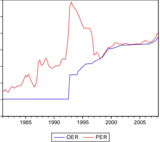
One consequence of the gradual liberalisation of the exchange rate was the significant reduction in the parallel exchange rate premium(Degefa, 2001). The graph below plots the official and parallel exchange rates to the USD.
Figure 2: Official and Parallel Exchange Rates (ETB per USD): 1981-2008 0 2 4 6 8 10 12 14 1985 1990 1995 2000 2005 OER PER
Real Effective Exchange Rate Index
In this paper, the real effective exchange rate is synonymous with the multilateral RER. In the traditional sense, however, an ‘effective’ exchange rate is one that accounts for the structure of protection. The drawback is that data requirements for its construction are ‘usually prohibitive’, while there is some evidence that it may not be significantly different from the usual measure(White and Wignaraja, 1992:1472). Therefore, this strategy is not pursued. A multilateral rate (basket of foreign currencies) is usually preferred to a bilateral rate since it tends to be a better representation of overall competitiveness.
There are several alternative methods to compute the real ‘effective’ exchange rate index (RER). Some important decisions need to be taken, which may or may not have an influence on the analysis. Therefore, we will justify each of these decisions in light of the purpose of this study.30The key choices include:
(a) Nominal rate: Official or Parallel;
(b) Averaging method: Geometric vs. Arithmetic;
(c) Weights: Time-varying vs. Fixed, and Total trade vs. Export vs. Import; (d) Trading partners: Criteria to choose which ones and how many;
(e) Price indices: CPI vs. PPI vs. WPI.
29
Seewww.imf.org/external/np/mfd/er/2008/eng/0408.htm. This means that the central bank (actively) intervenes in the foreign exchange market (by buying or selling foreign exchange) to allow a gradual devaluation of the birr.
The first dilemma arises in countries with a dual exchange rate system(White and Wignaraja,
1992:1472). In the case of Ethiopia, the parallel premium is only significant until 1997, after which it tracks fairly closely the official rate. Hence, the use of the official exchange rate seems to be appropriate, although robustness tests will inform us if there is a significant departure from the long-run relationship for the period pre-1997.
The geometric average is often seen as a superior method over the arithmetic averaging procedure, mainly due to its desirable symmetry and consistency properties(Hinkle and
Montiel, 1999:49-50). The arithmetic RER index is easier to compute, but it crucially depends on the choice of the base year. This is problematic to the extent that the base year is assumed to represent equilibrium in the assessment of exchange rate misalignment(Opoku-Afari,
2004). Moreover, the rate of change of the RER index (e.g. percent appreciation) will be sensitive to a shift of the reference period (re-basing). Finally, the arithmetic average gives larger weights to currencies that have significantly appreciated or depreciated in relation to the domestic currency.
The weighting scheme should reflect the relative importance of each country’s foreign currency and prices in the context of Ethiopia’s trade patterns(Hinkle and Montiel,
1999:97-8). Therefore, time-varying weights are often preferred to a fixed weighting scheme, since the former take into account changing trading patterns. For example, exchange rate fluctuations of the renminbi or the rupee (in relation to the birr) in the 1980s were not a significant determinant of Ethiopia’s external competitiveness, given the little volume of trade with China and India during that period. Nonetheless, China and India are increasingly important trade partners and this should be reflected in the weighting scheme.31Fixed weights may therefore misrepresent the structure of trade in some given period. The weights can be updated every period (e.g. moving average) or we could consider period averages. Various plots of the RER index suggest that there is very little variation with regard to alternative
weighting schemes.Li and Rowe (2007:39-41)reach the same conclusion for Tanzania, which
suggests that the changes in weights are dominated by changes in relative prices and/or nominal exchange rates. In terms of the determination of the weights, we could use total trade
30Li and Rowe (2007:33-45)
provide a detailed explanation of the concepts and issues involved in the construction a real exchange rate measure.
shares or export/import data alone. The choice should be guided by the objective of the study. Since we are interested in both export and import competitiveness, we use total trade shares to capture overall external competitiveness.
We have tried to include a large number of trading partners in order to obtain a representative sample. Although we started with the major 26 trading partners, three countries had to be dropped due to poor quarterly price data (Djibouti, USSR/Russia, and Yemen). These 23 partners represented 73 percent of total trade flows during the period 1981-2008. However, the RER index does not seem to be sensitive to the number of trading partners selected, perhaps because most currencies co-move with hard currencies (e.g. USD, EUR, GBP, YEN, etc.). The RER index for the 6 major trading partners during the 1981-2008 period (Germany, Italy, Japan, Saudi Arabia, UK, and US – which still represent over 50 percent of trade flows) is not significantly different from the main index. The plot shows very little variation, which is corroborated by the very high correlation coefficient between the two indices.
With regard to the price indices, it is not possible to find a precise empirical equivalent to the price of tradables and non-tradables(Edwards, 1989:87). Hence, it is common to proxy (domestic) non-tradable prices by the country’s consumer price index (CPI), while the
producer price index (PPI) or wholesale price index (WPI) are usually used to proxy (foreign) tradable prices. The argument is that the PPI and WPI are a better representation of the price of intermediate goods, since they mainly contain tradable goods. Despite the fact that the CPI contains some tradable goods, it is greatly influenced by the non-tradable activities, thus it is a good proxy. Some authors suggest the use of GDP deflators and unit labour costs, but these were not available for most of the countries on a quarterly basis.
Edwards (1989:90&126)suggests that the weighting scheme, the choice of trading partners, and the choice of price indices does not seem to have a significant impact on the construction of the RER index. The crucial decision is between bilateral and multilateral rates, which show considerable differences in behaviour (sometimes moving in opposite directions). A
multilateral real exchange rate index is preferred. Bearing in mind the discussion presented above, the RER index used in this study is computed as the geometric trade-weighted average of a basket of bilateral real exchange rates,
t= 1, ...,T i= 1, ...,n
whereNERis the bilateral nominal exchange rate index expressed in foreign currency per birr, whilePdandPfare domestic and foreign price indices, respectively (proxied by the CPI and PPI/WPI, as discussed above).32Both exchange rate and price indices are period
averages, with base 2000=100. The subscriptiidentifies the trading partner, andtthe time period. A total of 23 trading partners (n) were included in the construction of the REER index. Finally,wicorresponds to the weight of each trading partner, which is allowed to vary
with time (8 quarter moving average) to capture changes in trade patterns (e.g. the rise of China and India in the later part of the sample). The weights are computed as the share of each partner’s trade (exports plus imports) in the total volume of Ethiopia’s trade with the group of 23,
Long-Run Determinants
Several studies use net capital inflows as a determinant of the RER. For example,Edwards
(1989:136)uses the (lagged) ratio of net capital flows to GDP as a proxy for capital controls. However, there is a growing interest in the impact of specific capital inflows such as foreign aid, remittances and FDI. In fact, some level of disaggregation may be required, since it is unlikely that all inflows will induce the same impact, either in terms of magnitude or even sign. For example, remittances are likely to be biased towards the purchase of non-tradable (domestic) goods, while other flows may be predominantly used to purchase tradable goods.
The focus of this empirical exercise is on foreign aid inflows, both in the form of grants and concessional loans. For that purpose, most studies use net ODA flows (DAC) to proxy for foreign aid inflows. However, this paper argues that this is not a good measure for the reasons explained in previous chapters. Therefore we use data from the balance of payments. Foreign aid grants are listed as ‘public transfers’ in the current account, while foreign loans are a sub-item in the capital account. Due to data scarcity, remittances are proxied by ‘private transfers’