NBER WORKING PAPER SERIES
THE EXTENSIVE MARGIN OF EXPORTING PRODUCTS: A FIRM-LEVEL ANALYSIS
Costas Arkolakis Marc-Andreas Muendler
Working Paper 16641
http://www.nber.org/papers/w16641
NATIONAL BUREAU OF ECONOMIC RESEARCH 1050 Massachusetts Avenue
Cambridge, MA 02138 December 2010
We thank David Atkin, Thomas Chaney, Arnaud Costinot, Don Davis, Gilles Duranton, Jonathan Eaton, Elhanan Helpman, Kalina Manova, Gordon Hanson, Lorenzo Caliendo, Sam Kortum, Giovanni Maggi, Marc Melitz, Peter Neary, Jim Rauch, Steve Redding, Kim Ruhl, Peter Schott, Daniel Trefler and Jon Vogel as well as several seminar and conference participants for helpful comments and discussions. Roberto Avarez kindly shared Chilean exporter and product data for the year 2000, for which we report comparable results to our Brazilian findings in an online Data Appendix at URL econ.ucsd.edu/muendler/research. We present an extension of our model to nested CES in an online Technical Appendix at the same URL. Oana Hirakawa and Olga Timoshenko provided excellent research assistance. Muendler and Arkolakis acknowledge NSF support (SES-0550699 and SES-0921673) with gratitude. A part of this paper was written while Arkolakis visited the University of Chicago, whose hospitality is gratefully acknowledged. The views expressed herein are those of the authors and do not necessarily reflect the views of the National Bureau of Economic Research.
NBER working papers are circulated for discussion and comment purposes. They have not been peer-reviewed or been subject to the review by the NBER Board of Directors that accompanies official NBER publications.
© 2010 by Costas Arkolakis and Marc-Andreas Muendler. All rights reserved. Short sections of text, not to exceed two paragraphs, may be quoted without explicit permission provided that full credit, including © notice, is given to the source.
The Extensive Margin of Exporting Products: A Firm-level Analysis Costas Arkolakis and Marc-Andreas Muendler
NBER Working Paper No. 16641 December 2010
JEL No. F12,F14,L11
ABSTRACT
We use a panel of Brazilian exporters, their products, and destination markets to document a set of regularities for multi-product exporters: (i) few top-selling products account for the bulk of a firm's exports in a market, (ii) the distribution of exporter scope (the number of products per firm in a market) is similar across markets, and (iii) within each market, exporter scope is positively associated with average sales per product. Our data also show that firms systematically export their highest-sales products across multiple destinations. To account for these regularities, we develop a model of firm-product heterogeneity with entry costs that depend on exporter scope. Estimating this model for the within-firm sales distribution we identify the nature and components of product entry costs. We find that firms face a strong decline in product sales with scope but also that market-specific entry costs drop fast. Counterfactual experiments with globally falling entry costs indicate that a large share of the simulated increase in trade is attributable to declines in the firm's entry cost for the first product.
Costas Arkolakis
Department of Economics
Yale University, 28 Hillhouse Avenue P.O. Box 208268 New Haven, CT 06520-8268 and NBER costas.arkolakis@yale.edu Marc-Andreas Muendler Department of Economics, 0508 University of California, San Diego 9500 Gilman Drive
La Jolla, CA 92093-0508 and NBER
muendler@ucsd.edu
An online appendix is available at:
1
Introduction
Market-specific entry costs are an important ingredient in recent trade theory. Combined with firm heterogeneity, entry costs serve as a key explanation for exporter behavior and the size distribution of firms.1 After rounds of tariff reductions and drops in transport costs, local entry costs from technical barriers to trade and regulatory protection are thought to be major remaining impediments to trade (Baldwin 2000, Maskus and Wilson 2001).2 Micro-econometric estimates suggest that firm entry costs are a substantive fraction of export sales (Das, Roberts, and Tybout 2007, Maskus, Otsuki, and Wilson 2005). Market-specific fixed costs do not only limit firm entry, they also hinder the expansion of prolific multi-product exporters.
To study the nature and components of entry costs, we use comprehensive data on multi-product firms and their destinations. Beyond the extensive margin of firm presence, we decom-pose, destination by destination, an exporter’s sales into the extensive margin of the number of products—theexporter scope—and the remaining intensive margin of the exporter’s average sales per product, which we callexporter scale. We use a structural approach to quantify the relevance of multi-product exporters in a general-equilibrium framework for the first time. To do so, we separately identify sources of within-firm heterogeneity in product sales and economies of scope in local product entry costs. Based on our estimates, we assess the general-equilibrium effects of reduced market-specific fixed costs on the expansion of incumbent multi-product exporters and new exporters. Our simulations suggest that new products of incumbent exporters contribute less to bilateral trade than new exporters.
A number of key regularities emerge from our Brazilian exporter data and discipline the anal-ysis.3 First, a few top-selling products explain the bulk of a firm’s exports in a market, whereas wide-scope exporters sell their lowest-selling products in minor amounts.4 Second, within
des-1See for example Melitz (2003), Chaney (2008) and Eaton, Kortum, and Kramarz (2010).
2The World Bank estimates in itsGlobal Economic Prospects 2004report that trade facilitation would increase
world trade by approximately $377 billion overall, to which an improvement in the regulatory environment would contribute $83 billion and services sector infrastructure and e-business usage another $154 billion (World Bank 2003).
The World Trade Organization’sWorld Trade Report 2008asserts that “with respect to product standards, technical
regulations and sanitary and phytosanitary (SPS) measures, considerable opportunities exist for reducing trade costs” (WTO 2008, p. 149).
3To assess robustness for another country, we use panel data of Chilean exporters in 2000 (see ´Alvarez, Faruq,
and L´opez 2007). We find the regularities confirmed and estimates to be similar, and report them in our online Data Appendix.
4Bernard, Redding, and Schott (2010a) document a similar pattern for worldwide shipments by U.S. firms. We
tinations, there are few wide-scope and large-sales firms but many narrow-scope and small-sales firms. Third, within destinations, mean exporter scope and mean exporter scale are positively as-sociated. These three regularities occur repeatedly destination by destination. Comparing across destinations but within firms, we find that exporters are likely to sell their highly successful prod-ucts in many destinations and in large amounts. We interpret this body of regularities as evidence of heterogeneity in product efficiency, or consumer appeal, and as evidence of entry costs that vary by product and destination.
Guided by these facts, we propose a model of firm-product heterogeneity where firms face destination-specific entry costs for each of their products. The model rests on a single source of firm heterogeneity (productivity) and firms face declining efficiency in supplying their less suc-cessful products, similar to Eckel and Neary (2010) and Mayer, Melitz, and Ottaviano (2009).5 Our specification of local entry costs accommodates the cases of both economies or diseconomies of scope.6 The setup offers a tractable extension of the Melitz (2003) framework to multiple prod-ucts where the firm decides along three export margins: its presence at export destinations, its exporter scope at a destination, and its individual product sales at the destination.
We use our model’s structural implications to obtain novel estimates for parameters that govern separate entry cost components, fitting the within-firm heterogeneity under the first regularity. We check the fitted model’s prediction for the remaining two regularities across firms and show that the model approximates well the scope and sales distributions and generates the observed positive association between exporter scope and exporter scale. Estimates point to a strong decline in product efficiency with scope. So only highly productive firms choose a wide scope. But local entry costs exhibit economies of scope for the introduction of additional products within a market, consistent with the fact that wide-scope exporters sell their lowest-selling products in minor amounts.
Having parameterized the model, we simulate a 25-percent reduction in entry costs and their effect on global trade. We distinguish between a decline in firm entry costs for the first product and a decline in entry costs that a multi-product exporter incurs for additional export products. We
5Bernard, Redding, and Schott (2010a) develop a multi-product firm model with products that have idiosyncratic
country-specific demand shocks. Departing from CES demand, Eckel, Iacovone, Javorcik, and Neary (2010) study the firm’s investment in product appeal. Exporter scope is socially optimal in these models. Thomas (2010) proposes an agency approach to product adoption and documents inefficient variation in firm scope for detergent manufacturers across local markets in Western Europe.
6Seminal references on economies of scope are Panzar and Willig (1977) and (1981). Formally, there are economies
find that most of the simulated trade increase is due to falling entry costs for the first product— such as one-shot startup costs for information acquisition, the setup of certified and accredited testing facilities, investments in technology acquisition for export development, and perhaps brand marketing costs. In contrast, trade is less sensitive to falling entry costs for subsequent products— such as compliance with an individual product’s technical requirements, mandatory or voluntary product safety standards, and packaging and labelling procedures, or expenditures for extending marketing and the distribution network to additional products.
Overall, a simulated 25-percent reduction in entry costs only results in a less than 1-percent welfare increase. Firm entry costs are typically found to influence sales little because only small exporters around the entry threshold respond (Das, Roberts, and Tybout 2007, di Giovanni and Levchenko 2010). But incumbent exporters add products when entry costs fall, suggesting poten-tially salient changes to trade flows because multi-product exporters dominate trade. Our simula-tions show, however, that the elasticity of trade with respect to product entry costs is even smaller than with respect to firm entry costs. The reason for the surprisingly small contribution of the extensive margin of adding products is the estimated combination of strongly declining product efficiencies and economies of scope in local entry, so that even highly productive wide-scope ex-porters add only products that sell minor amounts. We confirm the small response at the extensive margin of exporting products also for a simulated 25-percent drop in variable trade costs.
Our analysis is related to an emerging literature that documents the dominance of multi-product firms in the economy and multi-product exporters in international trade (Bernard, Redding, and Schott 2010b, Goldberg, Khandelwal, Pavcnik, and Topalova 2010).7 Beyond existing evidence, we show systematic and recurrent exporter behavior market by market and the correlation of prod-uct sales within firms across markets.
For our model, we use a conventional demand system with constant elasticity of substitution (CES) and embed the Eckel and Neary (2010) production setup, by which firms can take up addi-tional products (away from their core competency) only at lower marginal efficiency. This setup implies that a firm’s product sales are perfectly correlated across the markets where a product is sold, which reflects features of our data but also distinguishes our approach from the stochastic
7Bernard, Jensen, and Schott (2009) show for U.S. trade data in 2000, for instance, that firms that export more than
five products at the HS 10-digit level make up 30 percent of exporting firms but account for 97 percent of all exports. In our Brazilian exporter data for 2000, 25 percent of all manufacturing exporters ship more than ten products at the internationally comparable HS 6-digit level and account for 75 percent of total exports. Similar findings are shared by
firm-product model of Bernard, Redding, and Schott (2010b and 2010a).8 Mayer, Melitz, and Ot-taviano (2009) analyze additional properties of the within-firm sales distribution through country-pair comparisons and explain them with an Eckel and Neary (2010) production setup under a varying demand elasticity.9
While intentionally parsimonious, our model is qualitatively consistent with the empirical reg-ularities under a set of mild and empirically confirmed restrictions on product efficiency and entry costs. Moreover, under the common assumption of Pareto distributed firm productivities, the model preserves desirable predictions of previous trade theory: at the firm level the model generates a to-tal sales distribution that is Pareto-shaped in the upper tail as in Chaney (2008), and at the country level it results in a general equilibrium gravity relationship resembling the one in Anderson and van Wincoop (2003) and Eaton and Kortum (2002).
Arkolakis, Costinot, and Rodr´ıguez-Clare (2009) show for a wide family of models, which includes ours, that conditional on identical observed trade flows these models predict identical ex-post welfare gains irrespective of firm turnover and product-market reallocation. Their find-ings also imply, however, that models in that family differ in their predictions for trade flows and welfare with respect to ex-ante changes in entry costs. Our model provides market-specific micro-foundations for these entry costs. The model’s tractable setup can be used to compute the impact of rich policy experiments on trade flows and welfare.
The organization of this paper is in six more sections. In Section 2 we describe the data and present key regularities. We introduce the general model in Section 3 and show how it generates the regularities. In Section 4 we derive equilibrium and bilateral trade under a Pareto distribution and adopt parametric functional forms for estimation. We obtain structural estimates of entry cost parameters in Section 5, and simulate their cross sectional predictions. Section 6 applies these estimates to simulate a drop in entry costs. Section 7 concludes.
8Incomplete correlation can readily be built into our model, using random sales shocks per product as developed
by Eaton, Kortum, and Kramarz (2010). The benchmark specification in Bernard, Redding, and Schott (2010b) makes product heterogeneity market specific so that product sales are uncorrelated across markets. For product sales covariation to be built into their model, a correlated distribution of product efficiencies would need to be specified.
9Feenstra and Ma (2008), Nocke and Yeaple (2006) and Dhingra (2010) study multi-product exporters but do not
2
Data
Our Brazilian exporter data derive from the universe of customs declarations for merchandize exports during the year 2000 by any firm. From these customs records, we construct a three-dimensional panel of exporters, their respective destination countries, and their export products at the Harmonized System (HS) 6-digit level. We briefly discuss the data sources and characteristics, and then present three main stylized facts that emerge from the data.
2.1
Data sources and sample characteristics
In our pristine exports data from SECEX (Secretaria de Com´ercio Exterior), product codes are 8-digit numbers (under the common Mercosur nomenclature), of which the first six digits coincide with the first six HS digits. We aggregate the monthly exports data to the HS 6-digit product, firm and year level. To relate our data to product-market information for destination countries and their sectors, we map the HS 6-digit codes to ISIC revision 2 at the two-digit level and link our data to World Trade Flow (WTF) data for the year 2000 (Feenstra, Lipsey, Deng, Ma, and Mo 2005). In 2000, our SECEX data for manufactured merchandize sold by Brazilian firms from any sector (including commercial intermediaries) reaches a coverage of 95.9 percent of Brazilian exports in WTF.
We restrict our sample to manufacturing firms and their exports of manufacturing products, removing intermediaries and their commercial resales of manufactures. The restriction to manu-facturing firms and their manufactured products makes our findings closely comparable to Eaton, Kortum, and Kramarz (2004) and Bernard, Redding, and Schott (2010a), for example. The group of manufacturing firms covers a substantial fraction of exports (81.7 percent of the WTF manu-factures exports).10 The resulting manufacturing firm sample has 10,215 exporters shipping 3,717 manufacturing products at the 6-digit HS level to 170 foreign destinations, and a total of 162,570 exporter-destination-product observations. Multi-product exporters sell more than 90 percent of all exports from Brazil.
10Exporter behavior in Brazil is strikingly similar to that in leading export countries such as France and the United
States (see our online Data Appendix). Appendix D.1 reports summary statistics and documents the dominance of multi-product exporters in total exports. In our online Data Appendix we also report findings from the complementary group of commercial intermediary firms and their exports of manufactures.
Brazil to USA Brazil to World 1 10 100 1000 10000
Exports (US$ Thsd fob)
1 2 4 8 16 32
Product Rank within Firm (HS 6−digit) 4−product Firms (159) 8−product Firms (36) 16−product Firms (4) 32−product Firms (1)
1
10
100
1000
10000
Mean Exports (US$ Thsd fob)
1 2 4 8 16 32
Product Rank within Firm (HS 6−digit) 4−product Firms (468) 8−product Firms (552) 16−product Firms (576) 32−product Firms (416)
Source:SECEX2000, manufacturing firms and their manufactured products.
Note: Products at the HS 6-digit level. World average in right-hand graph from pooling destinations where firms in a
given exporter-scope group ship.
Figure 1: Within-firm Sales Distribution
2.2
Three regularities
To describe the extensive margin of exporting products, we look at the number of products that a firm sells at each destination. We decompose a firmω’s total exports to destination d, td(ω), into
the number of productsGd(ω)sold atd(theexporter scopeind) and the average sales per export
productad(ω) ≡ td(ω)/Gd(ω)ind (theexporter scalein d). We elicit three major stylized facts
from the data at three levels of aggregation, moving from less to more aggregation.
Fact 1 Within firms and destinations, exports are concentrated in few top-selling products. Wide-scope exporters sell small amounts of their lowest-selling products.
Figure 1 depicts the distribution of sales of firms for different products within the firm.11 We consider firms with the same number of products and rank the products of each firm from top-selling (rank 1) to lowest-top-selling at a given destination. We then take the average across firms of each product at a given product rank and plot the logarithm of this value against the logarithm of the rank of the product. The figure depicts the results for manufacturers that sell exactly 4, 8, 16 or 32 products to Brazil’s top export destination in 2000, the United States, or worldwide over all destinations. The worldwide figures here treat the rest of the world as if it were a single destination (individual plots are similar destination by destination). The elasticity of individual product sales
11Bernard, Redding, and Schott (2010a) present evidence for U.S. firms’ sales worldwide comparable to the
with respect to the rank of the product is about -2.8 in the United States and -2.6 worldwide implying that sales fall sharply with rank. As expected, the contribution of the top-selling products in the total sales of firms is large: for firms with 32 products in the USA or Argentina, the top 3 products account, on average, for more than 85 percent of their total sales. This number is 76 percent for the world as one destination.
For shipments to the United States in Figure 1, the top-selling product (rank 1) sells on average US$ 38 million at 32-product firms but only US$ 2.2 million at 4-product firms.12 On average, the top-selling product of multi-product exporters accounts for 70 percent of their sales to a destination. For the lowest-selling product, in contrast, narrower-scope firms have far higher average sales per product than wide-scope exporters. The lowest-selling product of 32-products exporters to the United States, for instance, sells for merely US$ 12 in 2000 (rank 32) and 16-products exporters ship just US$ 77 of their lowest-selling product (rank 16). In contrast, the lowest-selling product of 8 and 4-products exporters (rank 8 and rank 4) sells for US$ 5,400 and US$ 67,000 respectively. Thus, the findings in Figure 1 suggest that wide-scope exporters have higher sales for their first product than narrow-scope firms. At the same time, wide-scope exporters tolerate lower sales for their lowest-selling products than narrow-scope firms.13
Fact 2 Within destinations, there are few wide-scope and large-sales firms but many narrow-scope and small-sales firms.
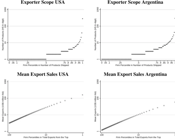
To graph the exporter scope distribution, we rank firms according to their exporter scopes in a destination market. The upper panel of Figure 2 plots exporter scope against the scope percentiles for Brazil’s top two exporting markets, the United States and Argentina. These plots too are sim-ilar for most Brazilian destinations. For instance, the median Brazilian exporter sells one or two products per destination and the mean number of products is around three to four products in in-dividual destinations (see also Table D.1 in the Appendix). Exporter scope is a discrete variable but the overall shape of the distributions approximately resembles that of a power-law distributed variable.
12There is considerable small-sample variability within single destinations so that top-product sales may not
gener-ally increase between firms with increasing scope. In Figure 1 for the United States, for instance, the (four) 16-product firms exhibit untypically low top-product sales compared to 8-product firms, whereas the (nine) 17-product firms do exhibit higher top-product sales compared to the (22) 9-product firms as expected. Destination aggregates do not exhibit such small-sample variability.
13Beyond Fact 1, Mayer, Melitz, and Ottaviano (2009) document that the slope of the graphs in Figure 1 is steeper
Exporter Scope USA Exporter Scope Argentina
1
10
100
1000
Number of Products (HS 6−digit)
0 .05 .1 .25 .5 .75 .8 .85 .9 .95 1 Firm Percentile in Number of Products Shipped
1
10
100
1000
Number of Products (HS 6−digit)
0 .05 .1 .25 .5 .75 .8 .85 .9 .95 1 Firm Percentile in Number of Products Shipped
Mean Export Sales USA Mean Export Sales Argentina
1
10
100
1000
Mean Exports (US$ million fob)
1 10
100
Firm Percentiles in Total Exports from the Top
1
10
100
1000
Mean Exports (US$ million fob)
1 10
100
Firm Percentiles in Total Exports from the Top
Source:SECEX2000, manufacturing firms and their manufactured products.
Note: Products at HS 6-digit level. In the lower panel, the left-most observations are all exporters; at the next percentile
are exporter observations with sales in the top 99 percentiles; up to the right-most observations with exporters whose sales are in the top percentile.
Figure 2: Exporter Scope and Export Sales Distributions
To graph the export sales distribution, we use cumulative plots in the lower panel of Figure 2. A cumulative plot naturally relates to later regularities for exporter scope and exporter scale. On the horizontal axis, we now group firms ator abovea given total exports percentile. At the origin, we cumulate all firms and plot mean total salest¯sd. Then we step one percentile to the right along the
horizontal axis and restrict the sample to all those firms that are in the top 99 percentiles, depicting mean total sales for that group of firms. We continue to move up in the total-exports ranking of firms and graph mean total sales by percentile group until we reach the top-percentile group of firms. Such a cumulative plot puts the emphasis on the mean exporter by percentile group and weights down deviant behavior of small-scale exporters.14 It is the signature of a power law
dis-14Introducing the marketing cost mechanism of Arkolakis (2010) is a straightforward extension of our model and
would allow us to match the size distribution of smaller firms as well. For our focus is on the multi-product firm, we abstain from an exploration of small-firm deviations.
USA Argentina p>=1 p>=50 p>=90 p>=95 100 1000 10000
Mean Exports/Product (US$ thsd fob)
1
2
4
16
64
Mean Number of Products
1 10
100
Firm Percentiles in Total Exports from the Top Mean Exporter Scope Firms’ Mean Product Scale
p>=1 p>=50 p>=90 p>=95 100 1000 10000
Mean Exports/Product (US$ thsd fob)
1
2
4
16
64
Mean Number of Products
1 10
100
Firm Percentiles in Total Exports from the Top Mean Exporter Scope Firms’ Mean Product Scale
World Seven Groups of Ten Countries
p>=1 p>=50 p>=90 p>=95 100 1000 10000
Mean Exports/Product (US$ thsd fob)
1
2
4
16
64
Mean Number of Products
1 10
100
Firm Percentiles in Total Exports from the Top Mean Exporter Scope Firms’ Mean Product Scale
top 1−10 top 51−60 top 61−70 top 1−10 top 11−20 top 61−70 1 100 1000 10000
Log Mean Exports/Product (US$ thsd fob)
1
2
4
16
64
Log Mean Number of Products
1 10
100
Log Firm Percentiles in Total Exports from the Top Mean Exporter Scope Firms’ Mean Product Scale
Source:SECEX2000, manufacturing firms and their manufactured products.
Note: World graph is based on pooling all markets. The groups-of-ten graph shows 70 markets (with 100 or more
Brazilian exporters), where markets are first ranked by total sales and then lumped to seven groups of ten countries by total-sales rank. Products at the Harmonized-System 6-digit level. Left-most observations are all exporters; at the next percentile are exporter observations with sales in the top 99 percentiles; up to the right-most observations with exporters whose sales are in the top percentile.
Figure 3: Mean Exporter Scale and Mean Exporter Scope
tribution that the log-log relationship in such a cumulative plot is linear. A power-law distribution implies that less frequent outcomes command a more than proportionate share of the total while the most frequent outcomes represent only a subordinate fraction. So there are few large-sales firms but many small-sales firms. (Plots of total exports against the total exports percentiles confirm the inference and resemble findings in Eaton, Kortum, and Kramarz (2010).) The plots for sales are similar across Brazilian destinations. Next we investigate the relationship between exporter scale and exporter scope.
Fact 3 Within destinations, mean exporter scope and mean exporter scale are positively associ-ated.
One might expect from Fact 1 that wide-scope firms would have low average sales per product because they adopt more products with minor sales. The opposite is the case. In Figure 3 we plot firms’ mean scope and scope-weighted mean exporter scale at a destination against these firms’ rank in total exports at that destination.15
The means in Figure 3 are computed in the same way as mean exports before and are linear decompositions of their counterparts in the lower panel of Figure 2, by construction. On the hori-zontal axis, we group firms at or above a given total exports percentile. At the origin, we cumulate all firms and plot their mean scopeG¯sdand the scope-weighted mean exporter scale¯asd so that the
product of the two means yields mean total salest¯sd. Then we move upwards in the total-exports
ranking of firms, percentile by percentile, dropping from the sample all those firms that are below the next higher total-exports percentile and depict mean exporter scope and mean average scale for the higher-ranked group of firms.
The log mean scope and log mean scale both increase in the firms’ log percentile. The increases are close to linear in the two export markets United States and Argentina and, on average, in the world (treating all destinations as a single market). This log-linear pattern is also visible in groups of ten similarly ranked destinations (70 destinations with at least 100 Brazilian exporters where destinations are first ranked by total sales and then lumped to seven groups of ten countries). Overall, Figure 3 strongly suggests that there is a systematically positive relationship between averageexporter scale and exporter scope.
2.3
Product shipments across destinations
Before we turn to a firm-level model, we investigate whether firms systematically sell their most successful products across destinations.16 We present evidence that a firm’s successful products in one market are also its leading products in other markets, and that a firm’s successful products reach a larger number of markets. To document systematic sales patterns by product and firm across markets, we use the United States as our reference country. The United States is Brazil’s top export destination in 2000.
15Scope-weighted mean exporter scale is[∑
ωGd(ω)ad(ω)]/ ∑ ωGd(ω) = ∑ ωtd(ω)/ ∑ gGd(ω). For unweighted
mean exporter scale, a similar positive association as depicted in Figure 3 arises. We present those figures and numer-ous additional results in our online Data Appendix.
16With the critique by Armenter and Koren (2010) and their balls-and-bins model of trade in mind, we pursue this
analysis also to show that systematic patterns in product entry are inconsistent with a simple stochastic model where exporters are just random collections of products.
Table 1: Overlaps between Reference Countries and Rest of World by Product Rank
Product Reference country: USA Reference country: Argentina
rank Overlap Overlap #Dest./ #Firms Overlap Overlap #Dest./ #Firms
in Ref. top prd. firm top prd. firm
country (1) (2) (3) (4) (5) (6) (7) (8) 1 .83 .83 8.9 2,280 .77 .77 7.8 3,071 2 .54 .77 13.0 1,033 .54 .76 10.7 1,672 4 .36 .73 18.9 368 .38 .67 14.2 797 8 .34 .69 24.1 137 .30 .63 18.5 307 16 .26 .59 24.3 63 .24 .54 22.6 136 32 .24 .53 30.2 22 .22 .50 29.7 48 64 .15 .49 38.9 10 .29 .40 35.9 19 128 .13 .69 42.4 5 .11 .33 43.8 12
Source:SECEX2000, manufacturing firms and their manufactured products.
Note: Destination counts in columns 3 and 7 are mean numbers of destinations to which firms with at least as many
products as reported for a rank ship. Overlap in columns 1 and 5 is the proportion of destinations that a product of reported rank reaches relative to the overall destination counts (in columns 3 and 7). Overlap in columns 2 and 6 is the proportion of destinations that the top-selling product of firms with at least as many products as reported for a rank reaches relative to the overall destination counts (in columns 3 and 7). Products at the HS 6-digit level, ranked by decreasing export value within firm in reference country. Sample restricted to firm-products that ship to reference country and at least one other destination.
First, within a firm, the leading products have systematically higher sales market by market. We number products within a firm and a destination by their rank in the firm’s local sales, assigning rank one to the firm’s top-selling product at a destination, rank two to the firm’s second-to-top product at the destination, and so forth. For each given HS 6-digit product that a firm sells in the United States we correlate the firm-product’s rank elsewhere with the firm-product’s U.S. rank. We find a correlation coefficient of .747 and a Spearman’s rank correlation coefficient of .837.17
Second, lower ranked products reach systematically fewer destinations. Table 1 documents that the number of destinations where a firm ships a product drops with the product’s rank in the reference country. Consider the top-ranked product in the United States for the 2,280 firms that ship at least one product to the United States (including single-product exporters to the United States). These firms reach 8.9 destinations on average and their top-selling product ships to 83 percent of the destinations that the firms reach with any product. Firms that sell at least two products in the United States reach on average 13.0 destinations but their second-ranked product only ships to a fraction of 54 percent of the destinations reached with any product. This fraction drops to
17When we repeat the exercise for Argentina (the second most important Brazilian export destination) as reference
country, we find an even higher correlation coefficient of .785 and a Spearman’s rank correlation coefficient of .860 for the same firm’s and same product’s ranks elsewhere.
36 percent for the fourth-ranked product for firms with at least 4 products in the United States and to 13 percent for the 128th ranked product. For Argentina as a reference country, the fraction drops systematically from 77 percent for the top-selling product to 11 percent for the 128th ranked product.
Finally, we report evidence that export scale per product is positively associated at the indi-vidual firm-product level, within industries and destinations (and not just across groups of firms as Fact 3 showed). For our sample of manufacturing exporters and their individual manufactured products, a regression of the log sales per product in a market on the seller’s log exporter scope in the same market, controlling for industry and destination fixed effects, documents a coefficient that is positive (0.072) and statistically significantly different from zero at the 1-percent level. So, wide-scope exporters in a destination also receive systematically higher revenues for each individ-ual product. This finding refutes the hypothesis that a firm is a random collection of products. For a random collection of products, the exporter scale would be independent of the exporter scope in a market.18
We turn to a model of exporting that generates the three stylized facts, and then revisit the data to empirically evaluate the derived relationships. The model strives to explain the behavior of multi-product exporters and to be quantitatively meaningful when matching the multi-product facts at successive levels of aggregation. The characteristic log-linear relationships in the data will motivate the choice of functional forms later.
3
A Model of Exporter Scope and Exporter Scale
Our model rests on a single source of firm heterogeneity. Firms sell one or multiple products in the markets where they enter. There are three key ingredients: a firm’s overall productivity that affects all products of the firm worldwide; firm-product specific efficiency that determines individual product sales worldwide; and local fixed entry costs that depend on the number of products that a firm sells in each destination market.
18If firms drew their product sizes from the same distribution (even if this distribution were truncated so that only a
fraction of the firm’s products made it to a given market), then the scale of each firm-product would not be related to the firm’s scope.
3.1
Consumers
There areN countries. We label the source country of an export shipment withs and the export destination with d. There is a measure of Ldconsumers at destination d. Consumers have
sym-metric preferences with a constant elasticity of substitution σ over a continuum of varieties. In our multi-product setting, a conventional “variety” offered by a firm ω from source countrys to destinationdis the product composite
Xsd(ω)≡ G∑sd(ω) g=1 xsdg(ω) σ−1 σ σ σ−1 ,
whereGsd(ω)is the number of products that firmωsells in countrydandxsdg(ω)is the quantity
of product g that consumers consume. In marketing terminology, the product composite is often called a firm’s product line or product mix. We assume that every product line is uniquely offered by a single firm, but a firm may ship different product lines to different destinations.
The consumer’s utility at destinationdis
( N ∑ k=1 ∫ ω∈Ωkd Xkd(ω) σ−1 σ dω ) σ σ−1 for σ > 1, (1)
whereΩkd is the set of firms that ship from source country k to destinationd. For simplicity we
assume that the elasticity of substitution across a firm’s products is the same as the elasticity of substitution between varieties of different firms.19
The representative consumer earns a wage wd from inelastically supplying her unit of labor
endowment to producers in country dand receives a per-capita dividend distribution πd equal to
her share1/Ld in total profits at national firms. We denote total income withYd = (wd+πd)Ld.
The consumer’s first-order conditions of utility maximization imply a product demand
xsdg(ω) = ( psdg Pd )−σ Td Pd , (2)
19In Appendix C (and in our companion paper Arkolakis and Muendler (2010) for a continuum of products), we
generalize the model to consumer preferences with two nests. The inner nest contains the products of a firm, which
are substitutes with an elasticity ofε. The outer nest aggregates those firm-level product lines over firms and source
countries, where the product lines are substitutes with a different elasticityσ ̸=ε. In this paper we setε =σ. The
general case ofε̸=σis fully consistent with the key regularities that we uncover but it introduces additional degrees
of freedom into the model that cannot be disciplined with three-dimensional firm-product-destination data such as ours.
Allanson and Montagna (2005) adopt a similar nested CES form to study the product life-cycle and market structure, and Atkeson and Burstein (2008) use a similar nested CES form in a heterogeneous-firms model of trade but do not consider multi-product firms.
wherepsdg is the price of productg in market d and we denote byTd the total spending of
con-sumer in countryd. In the calibration, we will allow for the possibility that total spendingTd is
different from country outputYdso that we use different notation for the two terms. We define the
corresponding ideal price indexPdas
Pd≡ ∑N k=1 ∫ ω∈Ωkd G∑kd(ω) g=1 pkdg(ω)−(σ−1)dω − 1 σ−1 . (3)
3.2
Firms
Following Chaney (2008), we assume that there is a continuum of potential producers of measure Jsin each source countrys. Productivity is the only source of firm heterogeneity so that, under the
model assumptions below, firms of the same typeϕfrom countrysface an identical optimization problem in every destinationd. Since all firms with productivityϕwill make identical decisions in equilibrium, it is convenient to name them by their common characteristicϕfrom now on.
A firm of typeϕ chooses the number of productsGsd(ϕ)to sell to a given marketd. The firm
makes each productg ∈ {1,2, . . . , Gsd(ϕ)}with a linear production technology, employing local
labor with efficiency ϕg. When exported, a product incurs a standard iceberg trade cost so that
τsd >1units must be shipped fromsfor one unit to arrive at destinationd. We normalizeτss= 1
for domestic sales. Note that this iceberg trade cost is common to all firms and to all firm-products shipping fromstod.
Without loss of generality we order each firm’s products in terms of their efficiency so thatϕ1 ≥
ϕ2 ≥ . . . ≥ ϕGsd. Ranking products by consumer appeal would generate isomorphic results for
within-firm product sales heterogeneity. A firm will enter export marketdwith the most efficient product first and then expand its scope moving up the marginal-cost ladder product by product. Under this convention we write the efficiency of theg-th product of a firmϕas
ϕg ≡
ϕ
h(g) with h
′(g)>0. (4)
We normalize h(1) = 1 so that ϕ1 = ϕ. We think of the function h(g) : [0,+∞) → [1,+∞)
as a continuous and differentiable function but we will consider its values at discrete pointsg = 1,2, . . . , Gsdas appropriate.20
20Considering the function in its whole domain allows us to express various conditions in a general form as we
will illustrate later on. The functionh(g)could be considered destination specific but such generality would introduce
By varying firm-product efficiencies, some products will sell systematically more across mar-kets (as empirically documented in Section 2.3 above). In turn, the assumption that the firm faces a drop in efficiency for each additional product when its exporter scope widens is a common as-sumption in multi-product models of exporters. Similar models are Eckel and Neary (2010), who define the product with the highest efficiency as the “core competency” of the firm, and Mayer, Melitz, and Ottaviano (2009). Nocke and Yeaple (2006), in contrast, assume that wider scope reduces efficiency for all infra-marginal products.
Related to the marginal-cost scheduleh(g)we define firmϕ’s product efficiency index as
H(Gsd)≡ G∑sd(ϕ) g=1 h(g)−(σ−1) − 1 σ−1 . (5)
This efficiency index will play an important role in the firm’s optimality conditions for scope choice. Since the marginal-cost schedule strictly increases in exporter scope, a firm’s product efficiency index strictly decreases as its exporter scope widens, resembling the insight from the stochastic firm-product model of Bernard, Redding, and Schott (2010a).
As the firm widens its exporter scope, it also faces a product-destination specific incremental local entry costfsd(g)that is zero at zero scope and strictly positive otherwise:21
fsd(0) = 0 and fsd(g)>0 for all g = 1,2, . . . , Gsd, (6)
wherefsd(g)is a continuous function in[1,+∞).
The incremental local entry cost fsd(g) accommodates fixed costs of production (e.g. with
0 < fss(g) < fsd(g)). In a market, the incremental local entry costs fsd(g) may increase or
decrease with exporter scope. But a firm’s local entry costs
Fsd(Gsd) =
∑Gsd
g=1fsd(g)
necessarily increase with exporter scope Gsd in countrydbecausefsd(g) > 0.22 We assume that
the incremental local entry costsfsd(g)are paid in terms of importer (destination country) wages
21Brambilla (2009) adopts a related specification but its implications are not explored in an equilibrium firm-product
model.
22As long as the firm’s first product causes a nontrivial fixed local entry cost, we do not need any additional fixed
local entry cost. In continuous product space with nested CES utility, in contrast, local entry costs must be non-zero at zero scope because a firm would otherwise export to all destinations worldwide (see Arkolakis and Muendler 2010, Bernard, Redding, and Schott 2010a).
so that Fsd(Gsd) is homogeneous of degree one in wd. Combined with the preceding varying
firm-product efficiencies, this local entry cost structure allows us to endogenize the exporter scope choice at each destinationd.
In summary, there are two scope-dependent cost components in our model, the marginal cost schedule h(g) and the incremental local entry cost fsd(g). Suppose for a moment that the
in-cremental local entry cost is constant and independent of g with fsd(g) = fsd. Then a firm in
our model faces diseconomies of scope because the marginal-cost scheduleh(g)strictly increases with the product indexg. But, if incremental local entry costs decrease sufficiently strongly with g, there could be overall economies of scope.
A firm with a productivity ϕ from country s faces the following optimization problem for selling to destination marketd
πsd(ϕ) = max Gsd,psdg Gsd ∑ g=1 ( psdg −τsd ws ϕ/h(g) ) ( psdg Pd )−σ Td Pd −Fsd(Gsd).
The firm’s first-order conditions with respect to individual pricespsdg imply product prices
psdg(ϕ) = ˜σ τsdwsh(g)/ϕ (7)
with an identical markup over marginal cost σ˜ ≡ σ/(σ−1) > 1forσ > 1.23 A firm’s choice of optimal prices implies optimal product sales for productg
psdg(ϕ)xsdg(ϕ) = ( Pd ˜ σ τsdws ϕ h(g) )σ−1 Td. (8)
Summing (8) over the firm’s products at destinationd, firmϕ’s optimal total exports to destination dare tsd(ϕ) = G∑sd(ϕ) g=1 psdg(ϕ)xsdg(ϕ) = ( Pd ˜ σ τsdws ϕ )σ−1 TdH ( Gsd(ϕ) )−(σ−1) , (9)
where H(Gsd) is a firm’s product efficiency index from (5). The term H(Gsd(ϕ))−(σ−1) strictly
increases inGsd(ϕ).
Given constant markups over marginal cost, profits at a destinationd for a firmϕ sellingGsd
are πsd(ϕ) = ( Pd ˜ σ τsdws ϕ )σ−1 Td σ H ( Gsd )−(σ−1) − Gsd ∑ g=1 fsd(g).
23Similarly, in continuous product space (Arkolakis and Muendler 2010) the optimal markup does not vary with
exporter scope for constant elasticities of substitution under monopolistic competition (even in the general case of
Note: Operating profits for the core product areπg=1(ϕ) = [P ϕ/(˜σ τ w)]σ−1T /σ. Combined incremental scope costs
z(g)≡f(g)h(g)σ−1strictly increase ingby Assumption 1, withf(0) = 0andh(1) = 1.
Figure 4: Optimal Exporter Scope
For profit maximization with respect to exporter scope to be well defined, we impose the following condition.
Assumption 1 (Strictly increasing combined incremental scope costs). Combined incremental scope costszsd(G)≡fsd(G)h(G)σ−1strictly increase in exporter scopeG.
Under this assumption, the optimal choice for Gsd(ϕ) is the largestG ∈ {0,1, . . .} such that
operating profits from that product equal (or still exceed) the incremental local entry costs:
( Pd ˜ σ τsdws ϕ h(G) )σ−1 Td σ ≥ fsd(G) ⇐⇒ πsdg=1(ϕ)≡ ( Pdϕ ˜ σ τsdws )σ−1 Td σ ≥ fsd(G)h(G) σ−1 ≡z sd(G). (10)
Operating profits from the core product are πsdg=1(ϕ), and operating profits from each additional productg areπsdg=1(ϕ)/h(g)σ−1.
Figure 4 depicts the choice of optimal exporter scope. A firm will keep widening its exporter scope as long as adding products does not reduce total profits. Equivalently, a firm will keep widening scope as long as incremental scope costs zsd(g) are weakly less than the firm’s core
operating profitsπsdg=1(ϕ). In this optimality condition, incremental local entry cost and costs from declining product efficiency enter multiplicatively and their product must increase in scope for a well defined optimum to exist. Thus, Assumption 1 is comparable to a second-order condition (for perfectly divisible scope in the continuum version of the model, Assumption 1 is equivalent to the second order condition). When Assumption 1 holds we will say that a firm faces overall diseconomies of scope.
We can express the condition for optimal scope more intuitively and evaluate the optimal scope of different firms. Firmϕexports fromstodiffπsd(ϕ)≥0. At the break-even pointπsd(ϕ) = 0,
the firm is firm is indif and only iferent between selling its first product to marketdand remaining absent. Equivalently, reformulating the break-even condition and using the above expression for minimum profitable scope, the productivity thresholdϕ∗sd for exporting fromstodis given by
(ϕ∗sd)σ−1 ≡ σfsd(1) Td ( ˜ σ τsdws Pd )σ−1 . (11)
In general, we can define the productivity thresholdϕ∗sd,G such that firms withϕ ≥ϕ∗sd,G sell at leastGsd products as ( ϕ∗sd,G )σ−1 ≡ σzsd(G) Td ( ˜ σ τsdws Pd )σ−1 , wherezsd(G)≡fsd(G)h(G)σ−1, or more succinctly, using (11), as
( ϕ∗sd,G )σ−1 = zsd(G) fsd(1) (ϕ∗sd)σ−1, (12)
under the convention thatϕ∗sd ≡ϕ∗sd,1. Note that if Assumption 1 holds thenϕ∗sd < ϕ∗sd,2 < ϕ∗sd,3 < . . . so that more productive firms introduce more products in a given market. So Gsd(ϕ) is a
step-function that weakly increases inϕ.
Using the above definitions, we can rewrite individual product sales (8) and total sales (9) as
psdg(ϕ)xsdg(ϕ) = σ fsd(1) ( ϕ ϕ∗sd )σ−1 h(g)−(σ−1) = σ zsd(Gsd(ϕ)) ( ϕ ϕ∗sd,G )σ−1 h(g)−(σ−1) (13) and tsd(ϕ) =σ fsd(1) ( ϕ ϕ∗sd )σ−1 H(Gsd(ϕ) )−(σ−1) . (14)
Proposition 1 If Assumption 1 holds, then for alls, d∈ {1, . . . , N}
• exporter scopeGsd(ϕ)is positive and weakly increases inϕforϕ ≥ϕ∗sd;
• total firm exportstsd(ϕ)are positive and strictly increase inϕforϕ≥ϕ∗sd.
Proof.The first statement follows directly from the discussion above. The second statement fol-lows because H(Gsd(ϕ))−(σ−1) strictly increases in Gsd(ϕ)and Gsd(ϕ) weakly increases in ϕ so
thattsd(ϕ)strictly increases inϕby (14).
The firm’s equilibrium choices for total sales tsd(ϕ) and the number of products soldGsd(ϕ)
determine itsexporter scalein marketd, asd(ϕ)≡ tsd(ϕ) Gsd(ϕ) =σ fsd(1) ( ϕ ϕ∗sd )σ−1 H(Gsd(ϕ) )−(σ−1) Gsd(ϕ) , (15)
conditional on exporting froms to d. In Section 2, we presented scope-weighted mean exporter scale. Exporter scale asd(ϕ) is tightly related to scope-weighted mean exporter scale: if asd(ϕ)
is a monotonic function of productivity then scope-weighted mean exporter scale is a monotonic function of productivity.24 In our model, it is easy to work with asd(ϕ)so we will characterize
its analytical properties to describe scope-weighted mean exporter scale. Under an additional restriction,asd(ϕ)increases in firm productivityϕand therefore also in firm total sales:
Restriction 1 (Strong overall diseconomies of scope).Combined incremental scope costszsd(G)≡
fsd(G)h(G)σ−1 strictly increase inGwith an elasticity
∂lnzsd(G)
∂lnG >1.
Restriction 1 is more stringent than Assumption 1 in that the restriction not only requireszsdto
increase withGbut that the increase be more than proportional. We can then state the following result.25
Proposition 2 Ifzsd(G)satisfies Restriction 1, then exporter scaleasd(ϕ)strictly increases inϕat
the thresholdsϕ=ϕ∗sd, ϕsd∗,2, ϕ∗sd,3, . . . , ϕ∗sd,G.
24To see this note that(t(ϕ) +x)/(G(ϕ) +y)≤x/y ⇐⇒ t(ϕ)/G(ϕ)≤x/y. So ift/Gdeclines then excluding
lower percentiles in scope-weighted mean exporter scale leads to increases in its value.
25Whereas the proposition demonstrates that the functiona
sd(ϕ)generically increases inϕ, this statement is not
true for allϕ. The simple reason is that the choice of products (the denominator of the functionasd(ϕ)) is a step
function that depends on combined incremental scope costszsd(G). The summation in the numerator ofasd(ϕ)is also
Proof.See Appendix A.1.
This proposition is particularly informative in situations where fsd(g) is a strictly decreasing
function. In such situations a highly productive firm adds many low-selling products because the firm can generate additional profits from these products asfsd(g)declines. So it is possible in such
situations that wide-scope firms would have low exporter scale. Restriction 1, however, suffices to guarantee that scale increases even iffsd(g)is a strictly decreasing function: it implies that the
efficiencies of marginal products decline so fast that only highly productive firms introduce them. These productive firms have high sales for their top selling products, which means that their overall scale is larger.26
The model can also parsimoniously generate the concentration of a firm’s sales in its core products. To do that we need to introduce an additional sufficient restriction onh(g).
Restriction 2 (Bounded firm-product efficiency).The marginal-cost scheduleh(·)results in boun-ded firm-product efficiency
limG→∞H(G)−(σ−1) =
∑∞
g=1h(g)−(σ−1) ∈(0,+∞).
A number of conventional real analysis tests (e.g. the root test or the ratio test, see Rudin 1976, ch. 3) can be used to determine whether the sum converges by looking at the limiting terms h(g)−(σ−1) asg → ∞. Formally, when this sum converges, the minimum share of a productg′ is bounded from below by the finite numberh(g′)−(σ−1)/∑+∞
g=1h(g)−(σ−1). Intuitively, Restriction 2
implies that the “core” products account for a significant share of total sales, which remain bounded even if many additional products are added.
4
Model Equilibrium and Model Predictions
To derive clear predictions for the model equilibrium we specify a Pareto distribution of firm pro-ductivity following Helpman, Melitz, and Yeaple (2004) and Chaney (2008). A firm’s propro-ductivity ϕ is drawn from a Pareto distribution with a source-country dependent location parameterbs and
a shape parameter θ over the support[bs,+∞)fors = 1, . . . , N. So the cumulative distribution
26Restriction 1 is a sufficient condition for the proposition. Examples can be found where Restriction 1 fails but
asd(ϕ)generically still increases inϕ. The result that scale increases with scope is not trivial and does not necessarily
generalize to other setups. In the Bernard, Redding, and Schott (2010a) multi-product model, for instance, it can be
function ofϕisPr = 1−(bs)θ/ϕθand the probability density function isθ(bs)θ/ϕθ+1, where more
advanced countries are thought to have a higher location parameter bs. Therefore the measure of
firms selling to countryd, that is the measure of firms with productivity above the thresholdϕ∗sd, is
Msd =Js(bs)θ/(ϕ∗sd) θ
. (16)
The probability density function of the conditional distribution of entrants is given by
µsd(ϕ) = θ(ϕ∗sd)θ/ϕθ+1 ifϕ ≥ϕ∗ sd, 0 otherwise. (17)
4.1
Equilibrium and the gravity equation of trade
Under the Pareto assumption we can compute several aggregate statistics for the model. We denote aggregate bilateral sales of firms from s to countryd withTsd. The corresponding average sales
per firm are defined asT¯sd, so thatTsd =MsdT¯sdand
¯ Tsd =
∫
ϕ∗sd
tsd(ϕ)µsd(ϕ)dϕ. (18)
Similarly, we define average local entry costs as
¯ Fsd =
∫
ϕ∗sd
Fsd(Gsd(ϕ))µsd(ϕ)dϕ.
To computeF¯sdin terms of fundamentals we need two further necessary assumptions.
Assumption 2 (Pareto probability mass in low tail). The Pareto shape parameter satisfies θ > σ−1.
Assumption 3 (Bounded local entry costs and product efficiency). Incremental local entry costs and product efficiency satisfy∑∞G=1fsd(G)−(˜θ−1)h(G)−θ ∈(0,+∞), whereθ˜≡θ/(σ−1).
Assumptions 2 and 3 guarantee that average sales per firm are positive and finite.
Proposition 3 Suppose Assumptions 1, 2 and 3 hold. Then for all s, d ∈ {1, . . . , N}, average sales per firm are a constant multiple of average local entry costs:
¯ Tsd = ˜ θ σ ˜ θ−1fsd(1) ˜ θ ∞ ∑ G=1 fsd(G)−(˜θ−1)h(G)−θ = ˜ θ σ ˜ θ−1 ¯ Fsd, (19) whereθ˜≡θ/(σ−1).
Proof.See Appendix A.2.
The share of total local entry costs in total exports F¯sd/T¯sd only depends on the model’s
param-eters θ andσ, even though local entry costs vary by source and destination country. So, despite firm-product heterogeneity, bilateral average sales can be summarized with a function only of the parametersθandσand the properties of average local entry costsF¯sd.
Finally, we can use definition (16) of Msd together with definition (11) of ϕ∗sd and
expres-sion (19) for average sales to derive bilateral expenditure shares of country d on products from countrys λsd = MsdT¯sd ∑ kMkdT¯kd = Js(bs) θ(w sτsd)−θfsd(1)− ˜ θF¯ sd ∑ kJk(bk)θ(wkτkd)−θfkd(1)− ˜ θF¯ kd , (20) whereθ˜≡θ/(σ−1), andfsd(1)− ˜ θF¯ sd = ∑∞ G=1fsd(G)− (˜θ−1)h(G)−θ by equation (19).
Remarkably, the elasticity of trade with respect to variable trade costs is −θ, as in Eaton and Kortum (2002) and Chaney (2008).27 Thus, our framework is consistent with bilateral gravity. The difference between our model, in terms of aggregate bilateral trade flows, and the framework of Eaton and Kortum (2002) is that fixed costs affect bilateral trade similar to Chaney (2008). Beyond previous work, we provide a micro-foundation as to how entry cost components affect aggregate bilateral trade through the weighted sum∑∞G=1fsd(G)−(˜θ−1)h(G)−θ. So our model offers a tool to
evaluate the responsiveness of overall trade to changes in individual entry cost components. The partial elasticity ηλ,f(g) of trade with respect to a product g’s entry cost component is
−(˜θ−1) times the product’s share in the weighted sum. To assess the relative importance of the extensive margin of exporting products, relative to firm entry with the core product, we can compare elasticities using the ratio
ηλ,f(g) ηλ,f(1) = fsd(g) −(˜θ−1)h(g)−θ fsd(1)−(˜θ−1) (21)
forg = 2, . . . and the standardizationh(1) = 1. Our model does not restrict this ratio to increase or decrease with g as a product becomes less important in the within-firm sales distribution. It therefore remains an empirical matter to quantify the importance of product entry relative to firm entry when entry costs change.
We can also compute mean exporter scope in a destination. For the average number of products to be finite we will need the necessary assumption that
27In our model, the elasticity of trade with respect to trade costs is the negative Pareto shape parameter, whereas it
Assumption 4 (Strongly increasing combined incremental scope costs). Combined incremental scope costs satisfy∑∞G=1zsd(G)−
˜
θ ∈(0,+∞).
This assumption is in general more restrictive than Assumption 1. It requires that combined incre-mental scope costsZ(G)do not just increase inG, but increase at a rate faster than1/θ˜.28
Mean exporter scope in a destination is
¯ Gsd = ∫ ϕ∗sd Gsd(ϕ)θ (ϕ∗sd)θ (ϕ)θ+1 dϕ= (ϕ ∗ sd) θ θ [∫ ϕ∗sd,2 ϕ∗sd ϕ−(θ+1)dϕ+ ∫ ϕ∗sd,3 ϕ∗sd,2 2ϕ−(θ+1)dϕ+. . . ] .
Completing the integration, rearranging terms and using equation (12), we obtain
¯ Gsd =fsd(1) ˜ θ∑∞ G=1zsd(G)− ˜ θ. (22)
The expression implies that mean exporter scope is invariant to destination market characteristics other than local entry costs. A priori there is no reason why mean exporter scope G¯sd should
be related to bilateral distance between s and d or to the size of the destination market. This implication resonates with the evidence of highly robust scope distributions across destinations as presented in Section 2.2.29
We turn to the model’s equilibrium. Notice that total manufacturing output of a country s equals its total sales across all destinations:
Ys=
∑N
k=1 λskTk. (23)
Additionally, Proposition 3 implies that a country’s total spending on fixed local entry costs is a constant (source country invariant) share of bilateral exports. This result implies that the share of wages in total income is constant (source country invariant). To see why observe that the share of net profits from bilateral sales is the share of gross variable profits in total sales 1/σ less the fixed costs paid and divided by total sales (˜θ−1)/θ σ˜ . Thus, using the result of Proposition 3, πsdLd/Tsd = 1/σ−(˜θ−1)/(˜θσ) = 1/(˜θ σ) = 1/(θσ˜). Total profits for country s are πsLs =
∑
kλskTk/(˜θσ), where
∑
kλskTk is the country’s total income by (23). So profit income and
28To see that, rearrange the expression to∑∞
G=1[fsd(G)h(G)σ−1]−
˜
θ =∑∞
G=1[Z(G)]− ˜
θand notice that the ratio
rule (see Rudin 1976, ch. 3) requires thatZ(G)increases at a rate faster than1/θ˜so that the sum converges.
29A regression of Brazil’s mean exporter scope on two main source-destination characteristics—market share and
import market size (see Appendix D.1)—shows that mean exporter scope responds relatively little to country charac-teristics, whereas the number of firms shipping to a destination is closely related to those characteristics (similar to Eaton, Kortum, and Kramarz 2004).
Table 2: Parametric Functional Forms
Condition Parameter values
Ass. 1 Strictly increasing combined incremental scope costs δ+α(σ−1)>0 Ass. 2 Pareto probability mass in low tail θ > σ−1
Ass. 3 Bounded local entry costs δ+α(σ−1)>(δ+1)/θ˜ Ass. 4 Strongly increasing combined incremental scope costs δ+α(σ−1)>1/θ˜ Restr. 1 Strong overall diseconomies of scope δ+α(σ−1)>1 Restr. 2 Bounded firm-product efficiency α(σ−1)>1
Note: Functional formsfsd(g) =fsd·gδandh(g) =gαby (25).
wage income can be expressed as constant shares of total income:
πsLs = 1 ˜ θσYs and wsLs = ˜ θσ−1 ˜ θσ Ys. (24)
We can now define an equilibrium in this economy, assuming for simplicity that trade is bal-anced with Yd = Td. (We will relax this assumption in the calibration.) Given τsd, Js, bs and
definitions (16) and (17) for alls, d= 1, . . . , N, an equilibrium is a set of firm-product consump-tion allocaconsump-tions for the representative consumer xsdg(ϕ) and prices and exporter scopes for the
representative firms [psdg(ϕ), Gsd(ϕ)] for g = 1, . . . , Gsd(ϕ) and ϕ ∈ Ωsd, and a set of wages
ws, such that (i) equation (2) is the solution of the representative consumer optimization program,
(ii) equations (7) and (10) solve the firm profit maximization programs, (iii) the current account balance condition (23) holds in every country s whereλsd is given by (20), and (iv)Pd andϕ∗sd,G
jointly satisfy equations (3) and (11) withYsgiven by equation (24).
4.2
Predictions for the cross section of firms
Parametrizing the model allows us to quantitatively match the patterns that we observe in the Brazilian data. Guided by the various log-linear relationships observed in Section 2.2 we set
fsd(g) = fsd·gδ forδ ∈(−∞,+∞),
h(g) = gα forα ∈[0,+∞). (25)
We first consider the necessary assumptions for equilibrium existence. Table 2 lists the condi-tions for the parametric funccondi-tions. Assumption 4 implies Assumption 1. It depends on the sign ofδ whether Assumption 3, which is needed to generate finite aggregate exports, implies Assumption 1